Multistep-Ahead Forecasting of Chlorophyll Concentration Based on Dynamic Collaborative Attention Network

Abstract

Multistep-ahead forecasting of chlorophyll concentration is of great significance in red tide early warning systems. Existing methods often neglect the potential adverse interactions between non-predictive variables and chlorophyll while failing to fully utilize the effective information in historical decoder units. To address these issues, this paper proposes a Dynamic Collaborative Attention Network (DCAN) model for chlorophyll concentration forecasting, which consists of two components: a Two-Stage Variable Embedding Network (TSVEN) and a Dynamic Attention Network (DyAN). The TSVEN can identify the non-predictive variables that have the most significant impact on chlorophyll changes and generate corresponding spatial vectors from them, thereby alleviating the information conflict between chlorophyll and non-predictive variables. The DyAN integrates a context attention module and a filtering gate mechanism. The former effectively extends the forecasting time range by dynamically retrieving historical decoder states, while the latter selectively integrates historical decoder information, thereby improving the reliability of model decisions and prediction accuracy. Experimental results based on real datasets show that the proposed model outperforms the current state-of-the-art methods in chlorophyll concentration forecasting tasks and exhibits good interpretability.

1. Introduction

Red tides are an abnormal ecological phenomenon that seriously threatens ecological balance and human safety, posing a significant threat to coastal economies and ecosystems [1]. They severely damage marine ecosystems, resulting in a sharp decline in biodiversity and ecological degradation. In marine ecosystems, chlorophyll concentration has been established as a key biochemical indicator characterizing the dynamic changes of ecosystems, and its spatial distribution characteristics and temporal variation patterns can effectively reflect the degree of water eutrophication and the level of primary productivity [2]. Studies have shown that this parameter is significantly positively correlated with phytoplankton biomass and can serve as a prospective early warning indicator for the risk of red tide outbreaks. It is generally recognized that red tides occur when the chlorophyll concentration exceeds 10 mg/m³, providing a scientific basis for the early monitoring of ecological disasters such as red tides [3]. In addition, chlorophyll concentration has a significant ecological coupling relationship with fish community structure, migration routes, and spawning ground distribution. Its spatiotemporal heterogeneity characteristics provide important ecological parameters for the site selection of artificial fishing grounds, the division of stock enhancement areas, and the assessment of fishery resources [4]. In practical applications, chlorophyll concentration forecasting is usually regarded as a complex multivariate time series forecasting problem whose core idea is to predict future chlorophyll concentration values using the chlorophyll concentration itself as well as various external variables such as temperature, pH value, and tidal patterns.

Currently, methods for predicting chlorophyll concentration can be roughly divided into two categories: traditional physicochemical analysis methods and data-driven methods. Traditional methods typically rely on dynamic models to explain and estimate chlorophyll concentration [5]. For instance, Ham et al. [6] successfully predicted the surface chlorophyll concentration in the South Pacific Ocean using a global marine biological prediction system based on an Earth system model. However, due to the high complexity and dynamic variability of marine water quality parameters, constructing accurate dynamic models remains highly challenging. The imperfection of physical parameterization processes in these models further limits prediction accuracy [2,6]. In recent years, with the rapid development of deep learning technologies, data-driven methods have been widely applied in the field of chlorophyll concentration prediction. Barzega et al. [7] adopted a hybrid model combining Long Short-term Memory (LSTM) networks and Convolutional Neural Networks (CNNs) to effectively predict short-term chlorophyll concentration in Lake Prespa, Greece. Multistep-ahead forecasting of chlorophyll concentration is of great practical significance, as it facilitates more forward-looking long-term decision-making. Recently, some researchers have applied the encoder-decoder framework to multistep-ahead forecasting tasks of chlorophyll concentration [8,9], and the introduction of attention mechanisms has further improved prediction performance [10]. However, due to the complex interactive relationships between observed data, current methods still have certain limitations. Firstly, existing models often overlook the potential adverse interactions between input variables, thereby affecting prediction accuracy. For example, the study by Li et al. [11] pointed out that the introduction of certain variables not only fails to improve prediction results but may even reduce model performance. Secondly, time series forecasting typically benefits from the effective utilization of recent historical information [12,13]. Nevertheless, current attention mechanisms mainly focus on the hidden states of the encoder, ignoring potentially useful information from previous decoder units. Therefore, incorporating the historical states of the decoder into the attention mechanism is expected to enhance the representation learning capability of the encoder-decoder structure.

In summary, the core objectives of this paper encompass two key aspects: first, to propose a novel encoding method to effectively mitigate the adverse interactions between chlorophyll and non-predictive variables; second, to design an attention mechanism for integrating the output information from the previous decoding unit into the current prediction process. To achieve these goals, this paper constructs a hierarchical Dynamic Collaborative Attention Network (DCAN) for the multistep-ahead forecasting task of chlorophyll concentration. The network framework adopts a bottom-up structure, consisting sequentially of a Two-Stage Variable Embedding Network (TSVEN) and a Dynamic Attention Network (DyAN). TSVEN assigns different weights to non-predictive variables in the first stage to reduce the interference of noise on model prediction and introduces a gated fusion module in the second stage to diminish the adverse interactions between chlorophyll and non-predictive variables. The input of DyAN is derived from the output of TSVEN, and its structure is an attention mechanism-based encoder-decoder framework. In the encoding phase, DyAN utilizes an LSTM network to capture complex dynamic dependencies in the time series. In the decoding phase, DyAN dynamically integrates the state information of previous decoders through a context attention mechanism, expanding the context horizon for current predictions. Additionally, DyAN incorporates a Filtering Gate Module (FGM) to selectively integrate information from the previous decoding unit into the state of the current unit, thereby further improving the accuracy of prediction results. The main contributions of this study can be summarized as follows:

• A novel interpretable prediction framework based on the DCAN is proposed, specifically designed for high-precision multistep-ahead forecasting of chlorophyll concentration. This framework not only significantly improves prediction performance but also provides interpretability of results, thereby enhancing the credibility of model and application value.
• A TSVEN is designed as a core component of DCAN. This network can effectively mitigate the potential negative impacts of non-predictive variables and achieve a reasonable balance of adverse interactions between chlorophyll and non-predictive variables.
• A DyAN is constructed as the upper structure of DCAN. This network can dynamically retrieve state information from previous decoders and use it as supplementary input for the current prediction stage, thereby further enhancing the predictive of model capability.
• Experiments conducted in the coastal waters of Xiamen demonstrate that the forecasting performance of DCAN is significantly superior to that of various benchmark models. Through visual analysis of the forecasting results, the effectiveness of incorporating state information from previous decoders in improving forecasting accuracy is verified.

2. Related Work

2.1. Chlorophyll Concentration Forecasting

As a crucial basis for marine ecological environment monitoring and disaster early warning (especially for red tide and green tide warnings), chlorophyll concentration has been regarded by many researchers as a key indicator for predicting the occurrence of red tides [14]. Traditional methods for chlorophyll concentration forecasting are mainly based on physicochemical analysis, relying on the chemical properties of water bodies, and simulating and predicting chlorophyll concentration using complex hydrodynamic models and water quality physicochemical forecasting models [6]. For example, Jin et al. [15] employed empirical models and machine learning methods to conduct long-term prediction of chlorophyll concentration changes in the Geum River Reservoir, South Korea. Subsequently, numerous studies have developed machine learning-based chlorophyll forecasting models, including Extreme Gradient Boosting (XGBoost), Random Forest (RF), and mixed-density networks [16,17,18]. This has provided unprecedented opportunities for analyzing the complex patterns of chlorophyll concentration. In recent years, deep learning methods such as Back Propagation Neural Networks (BPNN) [19], Convolutional Neural Networks (CNN) [7,20], and LSTM [7,9] have been widely applied in chlorophyll concentration forecasting research. Yao et al. [21] successfully achieved high-precision forecasting of chlorophyll concentration in the Yellow Sea and Bohai Sea of China through various deep learning models, verifying the effectiveness and application potential of these advanced technologies in this field. Yussof et al. [22] used LSTM and CNN models to predict Harmful Algal Blooms (HABs) events on the west coast of Sabah eight days in advance, and the results showed that the LSTM model has significant advantages in the accuracy of algal bloom forecasting.

2.2. Time Series Forecasting

Compared with traditional methods such as Holt-Winters [23] and Autoregressive Integrated Moving Average (ARIMA) [24], deep learning models exhibit stronger effectiveness in processing highly non-linear time series data in time series forecasting. As a result, deep learning models have been widely applied in various tasks such as traffic flow forecasting and stock market analysis [25]. Hu et al. [26] proposed a forecasting framework containing a multi-stage attention mechanism, which can adaptively capture the dynamic correlation between non-predictive sequences and target sequences. Du et al. [27] designed an attention mechanism-based encoder-decoder network for multistep-ahead forecasting of multivariate time series and verified its advantages over traditional methods. Shih et al. [28] introduced a temporal pattern attention mechanism to better capture temporal pattern features in multistep-ahead time series. Muralidhar et al. [12] pointed out that due to the dynamically changing nature of time series, the traditional encoder-centered attention mechanism is not the optimal choice in time series forecasting tasks.

3. Proposed Methods

3.1. Problem Definition and Symbols

Problem Definition 1: multistep-ahead forecasting of chlorophyll concentration.

Given historical time series data ${\left\{x_t\right\}}_{t=1}^T$ and ${\left\{y_t\right\}}_{t=1}^T$, where T denotes the past T time periods, $x_t$ = $x_t^1,x_t^2,\dots ,x_t^n$$\in {\mathbb{R}}^{1\times n}$ ($1\le t\le T$) represents the vector containing n non-predictive variables at time t, and $y_t$ denotes the chlorophyll concentration at the corresponding time. For multistep-ahead forecasting of chlorophyll concentration, the goal is to estimate the chlorophyll concentration for the next consecutive $\Delta$ time steps, i.e., ${\left\{{\widehat{y}}_t\right\}}_{t=T+1}^{T+\Delta }$ = ${\widehat{y}}_{T+1},{\widehat{y}}_{T+2},\dots ,{\widehat{y}}_{T+\Delta }$, where the output sequence should include predicted values for the future $\Delta$ time steps. $\Delta$ is referred to as the forecasting horizon, which can be adjusted according to specific task requirements. In summary, the multistep-ahead forecasting problem of chlorophyll concentration can be formulated as:

$${\left\{{\widehat{y}}_t\right\}}_{t=T+1}^{T+\Delta }=F({\left\{x_t\right\}}_{t=1}^T,{\left\{y_t\right\}}_{t=1}^T)$$

(1)

where $F(·)$ denotes a nonlinear mapping function. Based on this definition, this paper proposes a TSVEN, aiming to mitigate the adverse interactions between variables and thus address the second challenge mentioned earlier. Specifically, this paper introduces a dynamic fusion method that dynamically retrieves previous decoding states, performs nonlinear feature transformation on these signals, and selectively integrates the generated features into the hidden state of the current decoding unit. This process of retrieving and fusing previous decoding signals is referred to as contextual information fusion, as described in problem Definition 2.

Problem Definition 2: contextual information fusion Considering decoder unit i, its hidden state is denoted by ${\mathbf{h}}_i^d$. Assume that the source sequence ${\left\{\mathbf{h}\right\}}_{k=i-n}^{i-1}$ contains contextual information consisting of n hidden states, where the timestamps of all hidden states are earlier than the current decoder unit i. Contextual information fusion can be abstracted as a learning process that fuses the hidden state sequence ${\left\{\mathbf{h}\right\}}_{k=i-n}^{i-1}$ with the decoder state ${\mathbf{h}}_i^d$ through a set of nonlinear functions, thereby generating a contextual vector ${\tilde{\mathbf{h}}}_i^d$ with a higher-level semantic representation:

$$\mathbf{ho}=\xi \left({\left\{\mathbf{h}\right\}}_{k=i-n}^{i-1}\right)$$

(2)

$${\tilde{\mathbf{h}}}_i^d=\zeta (\mathbf{ho},{\mathbf{h}}_i^d)$$

(3)

where $\xi (·)$ is an information retrieval strategy, whose function is to aggregate the contextual information ${\left\{\mathbf{h}\right\}}_{k=i-n}^{i-1}$ into a semantic vector ${\mathbf{h}}_i^d$ with the same dimension as the target information $\mathbf{ho}$. $\zeta (·)$ denotes another nonlinear transformation function, which is used to map the vectors $\mathbf{ho}$ and ${\mathbf{h}}_i^d$ to a higher-level semantic space ${\tilde{\mathbf{h}}}_i^d$.

3.2. Dynamic Collaborative Attention Network

Based on problem Definition 1 and Definition 2, this paper proposes a novel multistep-ahead forecasting framework for chlorophyll concentration forecasting tasks, named DCAN. Its structure consists of two main components: TSVEN as the basic module, and the DyAN as the upper-level structure.

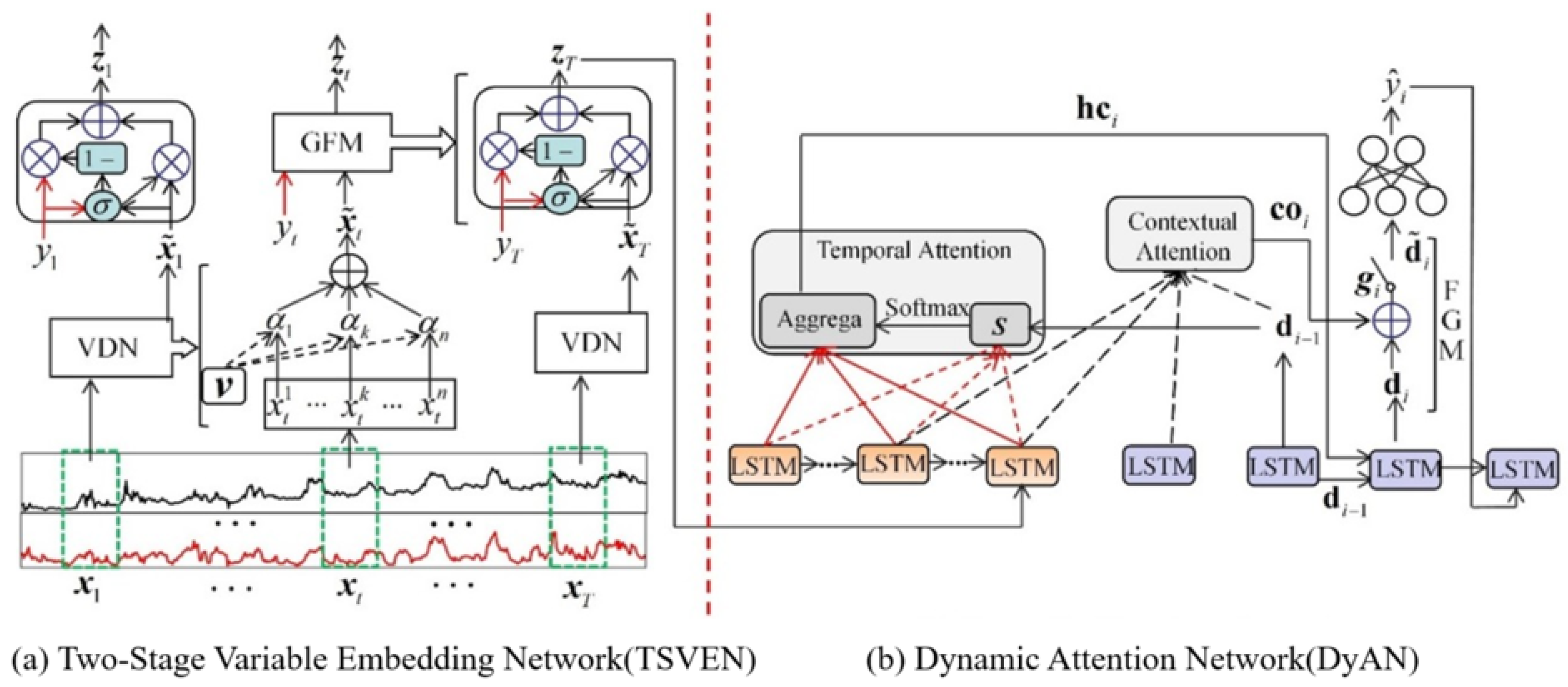
As shown in Figure 1a, TSVEN adopts a hierarchical deep neural network architecture, incorporating a Variable Distillation Network (VDN) at the bottom layer and integrating a Gated Fusion Module (GFM) at the upper layer. In the initial stage, TSVEN utilizes the VDN to abstract the input vector $x_t$ = {$x_t^1,x_t^2,\dots ,x_t^n$} ($1\le t\le T$) into a spatial semantic vector ${\tilde{x}}_t$, thereby effectively mitigating the negative impacts caused by non-predictive variables. In the subsequent stage, the GFM selectively fuses the spatial semantic vector ${\tilde{x}}_t$ with the chlorophyll concentration $y_t$ of the same period to generate a latent semantic sequence $z_t$, aiming to further suppress adverse interactions. As shown in Figure 1b, DyAN is a task-driven learning module whose structure integrates the attention mechanism with the encoder-decoder framework. The input of this module is the output of TSVEN. In the encoding phase, DyAN utilizes LSTM to capture the temporal dependencies among the semantic sequence ${\left\{z_t\right\}}_{t=1}^T$, and encodes them into a hidden state sequence ${\left\{{\mathbf{h}}_t\right\}}_{t=1}^T$. In the decoding phase, the temporal attention module performs weighted aggregation on the sequence ${\left\{{\mathbf{h}}_t\right\}}_{t=1}^T$ to generate a context vector $\mathbf{h}{\mathbf{c}}_i$. Additionally, DyAN introduces a context attention module and a Filtration Gate Module (FGM) to capture information from the previous decoding unit. Specifically, the context attention module dynamically integrates the state of the previous decoder to expand the perception range of the current decoding unit, while the FGM selectively fuses the semantic information output by the previous decoder into the hidden state of the current decoder, thereby enhancing the decision-making capability of the model. For ease of understanding, the technical details of TSVEN and DyAN will be elaborated in Section 3.2.1 and Section 3.2.2 respectively.

3.2.1. Two-Stage Variable Embedding Network

TSVEN incorporates a VDN to purify the features of non-predictive variables and designs a GFM for information fusion. In the following, this section will elaborate on the technical implementation process of TSVEN, starting from the structure and function of VDN and GFM.

The TSVEN is a hierarchical neural network architecture. Its core component at the bottom layer is the VDN, which is responsible for extracting variable features most relevant to the current task from $x_t$ = {$x_t^1,x_t^2,\dots ,x_t^n$}. This component effectively filters noise by enhancing the contribution of key variables to forecasting results while suppressing interference from non-predictive variables. VDN quantitatively evaluates the importance of each variable $x_t^k$ ($1\le k\le n$) in the context of $x_t$ = {$x_t^1,x_t^2,\dots ,x_t^n$} by assigning a weight score to it. Specifically, VDN first maps variables to a continuous vector space of specific dimensions to obtain their latent representations. Subsequently, each latent representation is scored, and the normalized exponential function is used to convert the scoring results into attention weights, thereby intuitively measuring the importance of each variable. Finally, based on these attention weights, VDN aggregates the latent representations into a vector representation with spatial semantics. This process is shown as follows:

$${\overline{x}}_t=tanh\left(\mathbf{Q}\left(v{x}_t\right)\right)$$

(4)

$$e_t=Softmax\left(w{\overline{x}}_t\right)$$

(5)

$${\tilde{x}}_t={\left[e_t{\left({\overline{x}}_t\right)}^T\right]}^T$$

(6)

where $v\in {\mathbb{R}}^m$ and $\mathbf{Q}\in {\mathbb{R}}^{m\times m}$ are learnable parameters during model training. ${\overline{x}}_t\in {\mathbb{R}}^{m\times n}$ denotes the information matrix, where its k-th column represents the latent representation of the non-predictive variable f in the m-dimensional continuous space. $w\in {\mathbb{R}}^m$ denotes the evaluation vector, which serves as a scoring function to evaluate variables. $Softmax(·)$ represents the normalized exponential function $e_t^i=exp\left({\upsilon }_i\right)/{\sum }_{k=1}^{n}exp\left({\upsilon }_k\right)$, whose role is to map the values of $e_t^i$ to the interval [0, 1]. $e_t\in {\mathbb{R}}^{1\times n}$ denotes the attention weight vector, where the value of a specific element $e_t^k$ ($1\le k\le n$) in $e_t$ indicates the importance of the variable $x_t^k$. ${(·)}^T$ denotes the matrix transposition operation. Finally, VDN fuses the information matrix ${\overline{x}}_t\in {\mathbb{R}}^{m\times n}$ into a spatial semantic vector ${\tilde{x}}_t$ through the attention weights.

Gated fusion module VDN only focus on non-predictive sequences, while ignoring the important signals contained in chlorophyll sequences. Therefore, the second stage of TSVEN aims to fuse information from both chlorophyll sequences and non-predictive sequences. Specifically, in the process of fusing semantics ${\tilde{x}}_t$ and variables $y_t$, GFM will actively screen information sources and quantify the proportion of information from semantics ${\tilde{x}}_t$ and variables $y_t$ in its output. This calculation process is shown as follows:

$$y_t=tanh\left(w_e{y}_t\right)$$

(7)

$$\mathbf{g}=\sigma ({\mathbf{W}}_y{y}_t+{\mathbf{W}}_x{\tilde{x}}_t)$$

(8)

$$z_t=\mathbf{g}\odot {\tilde{x}}_t+(1-\mathbf{g})\odot y_t$$

(9)

where $w_e\in {\mathbb{R}}^m$ is an embedding vector used to convert the target variable $y_t$ into a hidden representation with the same dimension as the abstract semantics ${\tilde{x}}_t$, thereby maintaining information consistency. ${\mathbf{W}}_y\in {\mathbb{R}}^{m\times m}$ and ${\mathbf{W}}_x\in {\mathbb{R}}^{m\times m}$ are parameters that can be learned during the training process. $\mathbf{g}\in {\mathbb{R}}^m$ is a control gate acting on the semantics ${\tilde{x}}_t$, $\sigma (·)$ is Sigmoid activation function, which is responsible for mapping the k-dimensional vector ${\mathbf{g}}^k$ ($1\le k\le m$) output by the control gate to the interval [0, 1]. Obviously, when ${\mathbf{g}}^k$ equals 0, the semantic vector $z_t$ retains only the information of at the corresponding position while discarding the content at the corresponding position in vector ${\tilde{x}}_t$.

3.2.2. Dynamic Attention Network

This paper designs a DyAN as the second core component of the DCAN model, aiming to explore the potential pattern features in time series data. As shown in Figure 1b, the input of DyAN is the sequence output by the TSVEN module, namely the sequence ${\left\{z_t\right\}}_{t=1}^T$. This component employs two structurally independent LSTM networks as its encoder and decoder, respectively.

DyAN encodes the output sequence of TSVEN LSTM network is one of the most successful improved models in Recurrent Neural Networks (RNNs). It can effectively alleviate the gradient vanishing problem existing in traditional RNNs. In terms of network structure, LSTM introduces a memory cell ${\mathbf{c}}_t$ for linear information transmission and designs three gating mechanisms: the forget gate ${\mathbf{f}}_t$, the input gate ${\mathbf{i}}_t$ and the output gate ${\mathbf{o}}_t$. These gating mechanisms jointly control the transmission path of information between different time steps and regulate the flow of information into and out of the memory cell. The specific calculation process is as follows:

$${\mathbf{i}}_t=\sigma \left({\mathbf{W}}_i{z}_t+{\mathbf{U}}_i{\mathbf{h}}_{t-1}+{\mathbf{b}}_i\right)$$

(10)

$${\mathbf{f}}_t=\sigma \left({\mathbf{W}}_f{z}_t+{\mathbf{U}}_f{\mathbf{h}}_{t-1}+{\mathbf{b}}_f\right)$$

(11)

$${\mathbf{o}}_t=\sigma \left({\mathbf{W}}_o{z}_t+{\mathbf{U}}_o{\mathbf{h}}_{t-1}+{\mathbf{b}}_o\right)$$

(12)

$${\mathbf{c}}_t={\mathbf{f}}_t\odot {\mathbf{c}}_{t-1}+{\mathbf{i}}_t\odot tanh\left({\mathbf{W}}_c{z}_t+{\mathbf{U}}_c{\mathbf{h}}_{t-1}+{\mathbf{b}}_c\right)$$

(13)

$${\mathbf{h}}_t={\mathbf{o}}_t\odot tanh\left({\mathbf{c}}_t\right)$$

(14)

where ${\mathbf{W}}_{*}\in {\mathbb{R}}^{m\times m}$, ${\mathbf{U}}_{*}\in {\mathbb{R}}^{m\times m}$ and ${\mathbf{b}}_{*}\in {\mathbb{R}}^m$ are automatically learned during the model training process. $z_t$ represents the output of TSVEN at time step t, and its specific calculation method is given by Equations (6) and (9). ${\mathbf{h}}_t\in {\mathbb{R}}^m$ denotes the output of the LSTM at time step t.

The decoding process of DyAN The decoding process of DyAN consists of two stages: the first stage is to establish the temporal dependency between the current forecasting and the input sequence, and the second stage is to realize the integration of context information (i.e., problem Definition 2). Taking decoder unit i as an example, this paper will explain these two operational steps in sequence. Here, ${\mathbf{d}}_i$ is used to denote the hidden state of decoder unit i.

In the first stage, this paper introduces a temporal attention mechanism as an information bridge connecting the encoder and decoder to establish associations between the current forecasting and each timestamp in the input sequence. Specifically, given a source input sequence ${\left\{h_t\right\}}_{t=1}^T$ and a task-related query vector $\mathbf{q}$, the attention mechanism assigns a corresponding attention score to each input item ${\mathbf{h}}_i$ ($1\le i\le \mathrm{n}$) based on the scoring function $\xi ({\mathbf{h}}_i,\mathbf{q})$. Subsequently, the score is normalized using the $Softmax$ function to obtain the corresponding attention weights. For decoder unit i, its query vector is derived from the hidden state ${\mathbf{d}}_{i-1}$ of the previous decoder unit. Therefore, the temporal attention mechanism is expressed as follows:

$$e_t=\xi ({\mathbf{h}}_t,{\mathbf{d}}_{i-1})={\mathbf{h}}_t\mathbf{W}{\left({\mathbf{d}}_{i-1}\right)}^T$$

(15)

$${\alpha }_t={\displaystyle \frac{exp\left(e_t\right)}{{\displaystyle \sum _{k=1}^T}exp\left(e_k\right)}}$$

(16)

$$\mathbf{h}{\mathbf{c}}_i=\sum _{t=1}^T{\alpha }_t\odot {\mathbf{h}}_t$$

(17)

where $\mathbf{W}\in {\mathbb{R}}^{m\times m}$ is a learnable parameter used to measure the importance of ${\mathbf{h}}_t$ to ${\mathbf{d}}_{i-1}$. $e_t$ represents the scoring result of the input item ${\mathbf{h}}_t$ by the scoring function, while ${\alpha }_t$ denotes the attention weight obtained through normalization of the score using the exponential function $e_t$. ⊙ indicates an element-wise multiplication operation, and $\mathbf{h}{\mathbf{c}}_i\in {\mathbb{R}}^m$ is the output result of the temporal attention mechanism, commonly referred to as the context vector.

In the second stage, the context attention mechanism is used to retrieve and summarize the state information of previous decoders, and transmit this summarized signal to the current forecasting. Meanwhile, the FGM is responsible for screening out valuable information from the signals output by the context attention mechanism and integrating it into the hidden state of the current decoder unit, thereby enhancing the ability of model to learn relevant information. For the first decoder unit, the context attention mechanism constructs an initial information pool queue based on the hidden states of the encoder, denoted as $D_1=\{{\mathbf{h}}_1,{\mathbf{h}}_2,\dots ,{\mathbf{h}}_T\}$. For subsequent decoder units i ($2\le i\le \Delta$), the information pool queue $D_{i-1}$ allows the current decoder state ${\mathbf{d}}_{i-1}$ to be added to the queue, and triggers the hidden state at the head of the queue to exit, so as to maintain a constant queue length. Subsequently, the context attention mechanism aggregates various pieces of information in the pool queue into a new context vector. The specific calculation process is shown as follows:

$${\mathbf{D}}_i=Matrix\left(D_i\right)$$

(18)

$$e_D={\mathbf{W}}_{D}tanh\left({\mathbf{Q}}_D{\left({\mathbf{D}}_i\right)}^T\right)$$

(19)

$${\beta }_D=Softmax\left(e_D\right)$$

(20)

$$\mathbf{c}{\mathbf{o}}_i={\left({\beta }_D{\mathbf{D}}_i\right)}^T$$

(21)

where $Matrix(·)$ denotes a matrix construction operation, which functions to convert the information queue $D_i$ into a context matrix ${\mathbf{D}}_i\in {\mathbb{R}}^{T\times m}$. ${\mathbf{Q}}_D\in {\mathbb{R}}^{m\times m}$ and ${\mathbf{W}}_D\in {\mathbb{R}}^m$ are learnable parameters in the model. The $Softmax(·)$ function converts the score $e_D$ into a T-dimensional attention weight vector, where the k-dimensional ($1\le k\le T$) represents the importance of the k-th hidden state in the information queue $D_i$. Subsequently, the context attention mechanism weights each element in the information queue $D_i$ and aggregates them into an information vector $\mathbf{c}{\mathbf{o}}_i$. This information vector provides additional historical context information for the current decoding unit $\mathbf{c}{\mathbf{o}}_i$. However, due to the cumulative effect of forecasting errors, this information vector may contain noise. To address this, DyAN introduces a FGM to filter the information in the vector $\mathbf{c}{\mathbf{o}}_i$ and integrate the purified signal into the hidden state of the current decoding unit. This process is shown as follows:

$${\mathbf{s}}_i=\sigma [{\mathbf{W}}_d{\mathbf{d}}_i:{\mathbf{W}}_c\mathbf{c}{\mathbf{o}}_i]$$

(22)

$$\mathbf{c}{{\mathbf{o}}^{\prime }}_i=tanh\left({\mathbf{U}}_c\mathbf{c}{\mathbf{o}}_i\right)$$

(23)

$${\mathbf{u}}_i={\mathbf{s}}_i\odot \mathbf{c}{{\mathbf{o}}^{\prime }}_i$$

(24)

$${\tilde{\mathbf{d}}}_i={\mathbf{U}}_s[{\mathbf{U}}_d{\mathbf{d}}_i:{\mathbf{u}}_i]$$

(25)

where $[:]$ denotes the concatenation operation of vectors. ${\mathbf{W}}_{*}\in {\mathbb{R}}^{m\times m}$ and ${\mathbf{U}}_d\in {\mathbb{R}}^{m\times m}$ are learnable parameters. ${\mathbf{s}}_i\in {\mathbb{R}}^{2m\times 1}$ represents the filtering gate, whose k-dimensional value ${\mathbf{s}}_i^k$ ($1\le k\le 2m$) is mapped to the interval [0, 1] through a logistic function. ${\mathbf{U}}_c\in {\mathbb{R}}^{2m\times m}$ and ${\mathbf{U}}_s\in {\mathbb{R}}^{m\times 3m}$ are learnable weights. $\mathbf{c}{{\mathbf{o}}^{\prime }}_i\in {\mathbb{R}}^{2m\times 1}$ is the hidden representation of the information vector $\mathbf{c}{\mathbf{o}}_i$, and its dimension is consistent with that of the filtering gate. When the k-dimensional information of the vector $\mathbf{c}{{\mathbf{o}}^{\prime }}_i$ is helpful to improve the representation ability of the decoder state, the corresponding position of the filtering gate will be activated to 1; otherwise, it will be suppressed to 0. The continuous value-taking characteristic of the filtering gate within the interval [0, 1] enables the FGM to screen the information in $\mathbf{c}{\mathbf{o}}_i$, thereby obtaining a more accurate semantic representation.

3.2.3. Joint Forecasting

As mentioned earlier, the temporal attention mechanism and context attention mechanism are responsible for generating the context vector $\mathbf{h}{\mathbf{c}}_i$ and information vector $\mathbf{c}{\mathbf{o}}_i$ required by the decoder unit, respectively. Subsequently, DyAN first updates the current hidden state ${\mathbf{d}}_i$ of decoder unit i based on the context vector $\mathbf{h}{\mathbf{c}}_i$ and the forecasting output ${\widehat{y}}_i$ from the previous time step. Then, the FGM screens the information vector $\mathbf{c}{\mathbf{o}}_i$ and fuses the filtered valid information into the current hidden state ${\mathbf{d}}_i$ to obtain the final semantic representation ${\tilde{\mathbf{d}}}_i$. This process is shown as follows:

$$\mathbf{h}{\mathbf{c}}_i=TA({\mathbf{h}}_1,{\mathbf{h}}_2,\dots ,{\mathbf{h}}_T)$$

(26)

$$\mathbf{c}{\mathbf{o}}_i=CA\left({\mathbf{D}}_i\right)$$

(27)

$${\mathbf{d}}_i=LSTM([{\widehat{y}}_{i-1}:\mathbf{h}{\mathbf{c}}_i],{\mathbf{d}}_{i-1})$$

(28)

$${\tilde{\mathbf{d}}}_i=FG({\mathbf{d}}_i,\mathbf{c}{\mathbf{o}}_i)$$

(29)

where $TA(·)$ denotes temporal attention, whose calculation process is shown in Equation (17). ${\mathbf{D}}_i$ is the context information matrix corresponding to decoder unit i, and $CA(·)$ represents context attention. The construction method of ${\mathbf{D}}_i$ and the calculation process of $CA(·)$ can be referred to in Equation (21). $LSTM(·)$ is a long short-term memory network unit, and its calculation process can be derived by replacing $z_t$ and ${\mathbf{h}}_{t-1}$ in Equation (14) with $[{\widehat{y}}_{i-1}:\mathbf{h}{\mathbf{c}}_i]$ and ${\mathbf{d}}_{i-1}$, respectively. $FG(·)$ denotes the filtering gate, whose calculation process is shown in Equation (25). Finally, the feedforward network learns the forecasting result from the hidden state ${\tilde{\mathbf{d}}}_i$ of decoder i, and the specific calculation process is as follows:

$${\widehat{y}}_i={\mathbf{W}}_p{\tilde{\mathbf{d}}}_i$$

(30)

where ${\mathbf{W}}_p\in {\mathbb{R}}^m$ denotes a learnable parameter.

4. Experimental Results and Analysis

4.1. Dataset

To verify the applicability of the DCAN model in multistep-ahead forecasting of chlorophyll concentration, the dataset used in this study consists of in-situ buoy monitoring data from a single station. The monitoring buoy is deployed in the Eastern Water off the coast of Xiamen City, Fujian Province, China, with its geographical coordinates at (${118}^{\circ }{04}^{\prime }$ N, ${24}^{\circ }{53}^{\prime }$ S). The DCAN model is systematically analyzed, and its forecasting results are compared with those of current mainstream advanced baseline methods. The dataset used in the experiments covers various relevant variables from January 2009 to August 2011, including meteorological conditions, water quality parameters, and nutritional status, with a time resolution of 30 min. However, due to factors such as instrument failures, 9974 time-series data points with complete records were finally obtained. Each data point includes 9 variables: chlorophyll, sea surface temperature, dissolved oxygen, saturated dissolved oxygen, tide, air temperature, standard atmospheric pressure and two wind speed components (Wind_u and Wind_v). In this study, the first 80% of the dataset was used for model training, and the remaining 20% was used for evaluating the model performance. It should be noted that in the experiment, the entire dataset was divided into two mutually exclusive parts: the training set and the test set. The training set was used to train the model to obtain the optimal parameters. Subsequently, the trained model was applied to the test set to evaluate its performance on unseen data. Both the training and test sets required all 9 variables as input, while the output was solely the chlorophyll concentration. The input length was 24 time points, with each time point containing data for all 9 variables. The output length was also 24, corresponding to the chlorophyll concentration predictions for 24 consecutive future time points.

4.2. Baselines Approaches

To evaluate the performance of the DCAN model in chlorophyll concentration forecasting, this paper compares it with advanced baseline methods based on real-world datasets. The details are as follows:

• DA-TLSTM: Hu et al. [26] proposed a multistep-ahead forecasting model for multivariate time series based on a multi-stage attention network.
• MTSMFF: Du et al. [27] applied this model to multivariate time series forecasting tasks. Based on practical application effects, MTSMFF has been proven to outperform traditional methods such as ARIMA and SVR.
• TPA-LSTM: Shih et al. [28] proposed a single-step forecasting model for multivariate time series. This model converts time series into different “frequency domains” by introducing a set of filters, thereby extracting stable temporal feature patterns.
• DSTP-RNN: Liu et al. [29] proposed a multistep-ahead forecasting model for multivariate time series, which can simultaneously capture the spatial correlations between variables and the temporal dependencies within sequences.

4.3. Evaluation Metrics and Parameters

To evaluate the predictive performance of the model, this paper adopts Root Mean Square Error (RMSE) and Mean Absolute Error (MAE) as evaluation metrics. RMSE reflects the mean squared deviation between the predicted results and the true values, while MAE represents the average absolute deviation between the predicted values and the true values. In general, the closer the values of these two metrics are to 0, the higher the forecasting accuracy of the model. The specific calculation formulas for MAE and RMSE are shown as follows:

$$MAE={\displaystyle \frac{1}{\Delta }}\sum _{t=1}^{\Delta }\left({\displaystyle \frac{1}{N}}\sum _{i=1}^N|{\widehat{y}}_t^i-y_t^i|\right)$$

(31)

$$RMSE={\displaystyle \frac{1}{\Delta }}\sum _{t=1}^{\Delta }\left(\sqrt{{\displaystyle \frac{1}{N}}\sum _{i=1}^N{({\widehat{y}}_t^i-y_t^i)}^2}\right)$$

(32)

where $\Delta$ denotes the length of the model output sequence. N is the total number of samples in the dataset. $y_t^i$ ($1\le i\le N$,$1\le t\le \Delta$) represents the true value of sample i at time step t, and ${\widehat{y}}_t^i$ denotes the corresponding predicted value by the model.

During the training process, the DCAN model and its comparative baseline methods adopted the same parameter initialization strategy. Specifically, all model parameters were initialized based on a truncated normal distribution. The Adam algorithm [30] was used in the model optimization process, with the learning rate set to 0.0001. In addition, for deep learning models, this paper conducted a grid search on the selection of the number of hidden units, with the search range being {10, 15, 20, 25, 30, 35, 40}, to determine the optimal LSTM structure parameters that can achieve the best performance. For the TPA-LSTM model, the grid search range for the number of convolution kernels was set to {24, 48, 64, 128} to determine the optimal configuration. During the training process, both the DCAN model and the baseline methods used RMSE as the loss function, and optimized the model parameters by minimizing this loss function.

4.4. Analysis of Experimental Results

4.4.1. Comparison with Baseline Methods

To ensure the fairness of the experiment, the input length for both the DCAN model and all baseline methods was uniformly set to 24 ($T=24$). The forecasting horizons were selected sequentially from the set {1, 3, 6, 12, 24} and increased incrementally. Since the time resolution of dataset is 30 min, the specific time units are 0.5 h, 1.5 h, 3 h, 6 h, and 12 h. This means that when the predicted horizon value is 24, the model continuously predicts chlorophyll concentrations for the next 720 min.

Table 1. Performance comparison of baseline methods across different time points (time resolution: 0.5 h).

Methods	0.5 h		1.5 h		3 h		6 h		12 h
	MAE	RMSE	MAE	RMSE	MAE	RMSE	MAE	RMSE	MAE	RMSE
DA-TLSTM	0.401	0.580	0.481	0.704	0.546	0.744	0.617	0.783	0.656	0.812
MTSMFF	0.429	0.569	0.570	0.773	0.801	0.953	0.889	1.039	0.969	1.152
DSTP-RNN	0.386	0.569	0.479	0.701	0.533	0.723	0.576	0.803	0.752	0.902
TPA-LSTM	0.431	0.561	0.598	0.747	0.666	0.832	0.718	0.893	0.785	0.977
DyAt-Nets	0.429	0.593	0.513	0.711	0.590	0.788	0.768	0.948	0.8205	0.967
DCAN	0.388	0.530	0.485	0.692	0.538	0.678	0.611	0.745	0.621	0.773

Note: Bold indicates the best result, and the underline indicates the second-best result.

presents the forecasting results of each method under different time points, with the optimal results highlighted in bold. As shown in the table, the DCAN model generally outperforms the baseline methods in the chlorophyll concentration forecasting task. In addition, the data in the table indicate that as the forecasting horizon increases along the set {0.5 h, 1.5 h, 3 h, 6 h, 12 h}, the forecasting accuracy of both the DCAN model and the baseline methods decreases to varying degrees. TPA-LSTM is a time-series modeling method for single-step-ahead forecasting; thus, a separate model needs to be trained for each future time point to be predicted. However, time-series data typically exhibit highly non-linear and time-varying characteristics, and uncertainties increase over time, making it difficult to accurately predict distant time points from the input observation period. In contrast, methods such as DCAN, DA-TLSTM, MTSMFF, DSTP-RNN and DyAt-Nets can complete the entire forecasting task in a single training process. However, these methods usually rely on the forecasting result of the previous step as part of the current input during the decoding stage, leading to the gradual accumulation of forecasting errors over time. Therefore, error accumulation becomes the main reason for the decline in the forecasting performance of these methods. Notably, according to the results in Table 1, DCAN still outperforms other baseline methods in most forecasting scenarios, indicating that it maintains relatively stable forecasting performance even when the forecasting horizon expands.

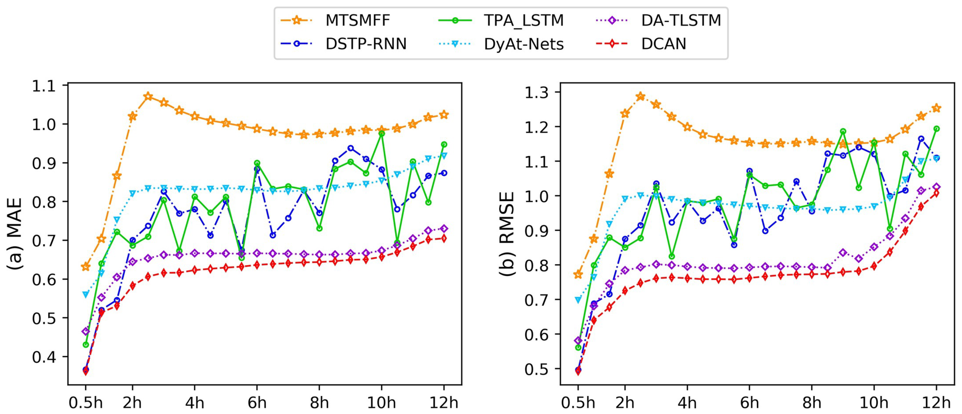
To more intuitively compare the performance of the aforementioned models, this paper takes the specific forecasting scenario of $\Delta =24$ as an example and conducts a visual analysis of the performance of each method across different horizons. As shown in Figure 2, the x-axis represents different forecasting time points within the forecasting range, and the y-axis (μg/L) denotes the MAE or RMSE of each method at the corresponding forecasting points. Taking the red curve as an example, the point with a value of 0.5 h on the x-axis represents the first forecasting time step when the horizon is set to 12 h, and the value on the y-axis corresponds to the MAE or RMSE of DCAN at this forecasting point. From the visualization results, it can be observed that DCAN demonstrates stronger competitiveness in the multistep-ahead forecasting task of chlorophyll concentration compared to mainstream deep learning methods such as MANet, MTSMFF, DSTP-RNN, TPA-LSTM and DyAt-Nets.

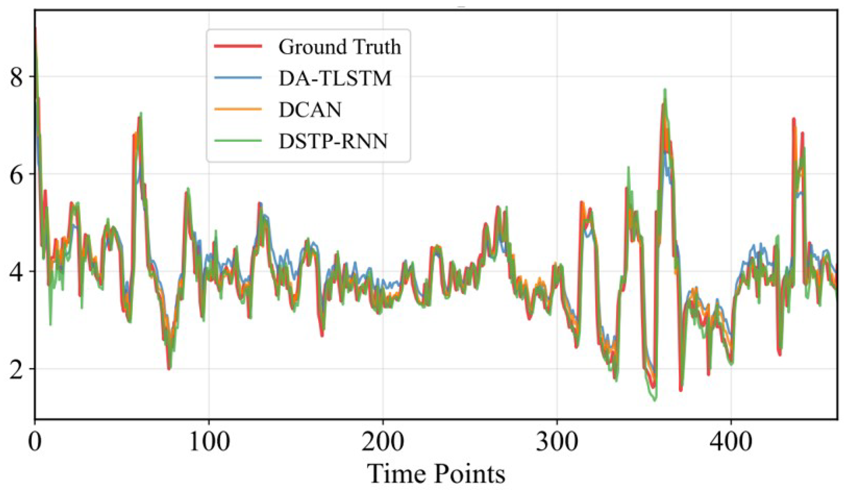
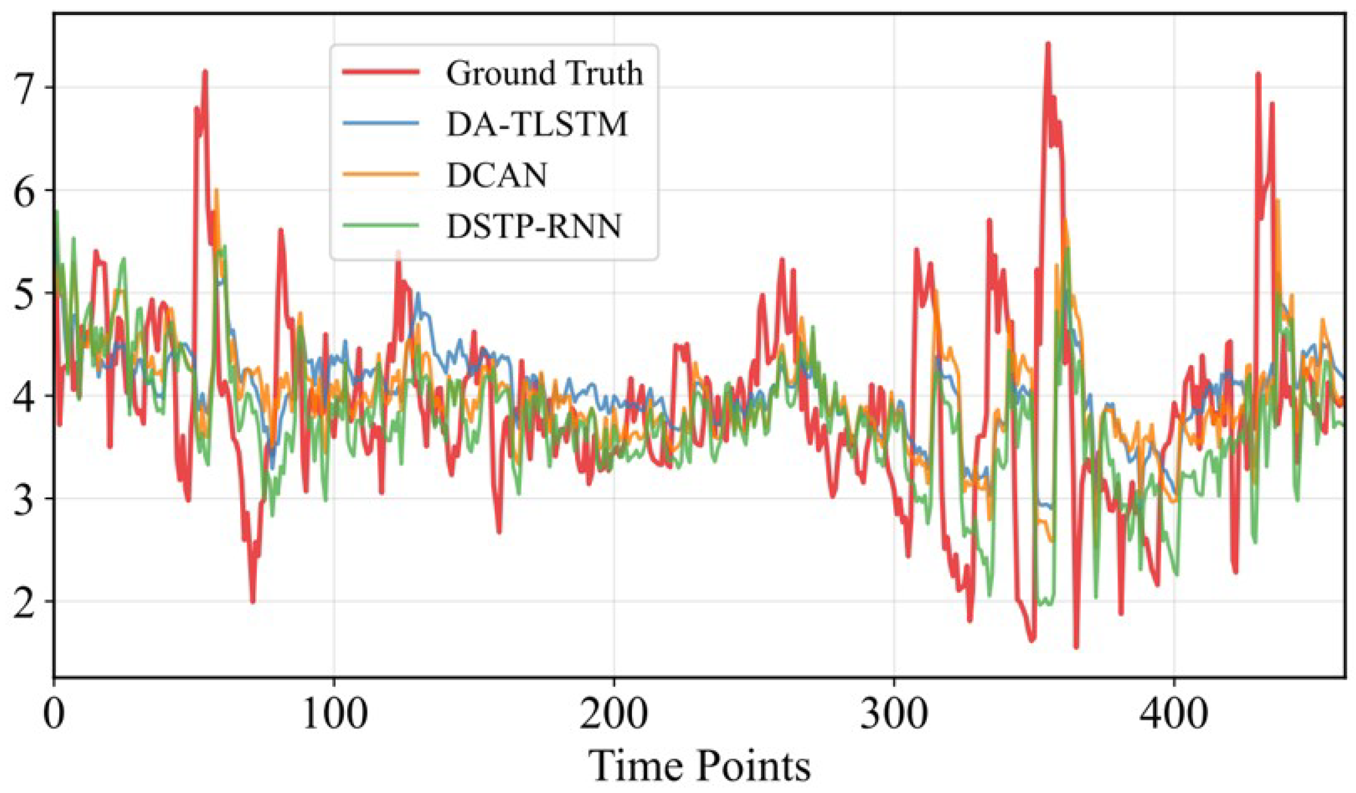
To comprehensively evaluate the predictive performance of model across different time horizons. Specifically, this study extracted data every 120 min (i.e., 2 h) to enable predictions for the next 48 h (2 days). To visually and quantitatively assess the model performance, this paper first present

Table 2. Performance comparison of baseline methods across different time points (time resolution: 2 h).

Methods	2 h		6 h		12 h		24 h		48 h
	MAE	RMSE	MAE	RMSE	MAE	RMSE	MAE	RMSE	MAE	RMSE
DA-TLSTM	0.449	0.803	0.544	0.808	0.623	1.024	0.691	1.117	0.721	1.170
MTSMFF	0.479	0.805	0.580	0.902	0.700	1.056	0.791	1.134	0.841	1.252
DSTP-RNN	0.458	0.800	0.584	0.906	0.633	0.991	0.718	1.056	0.751	1.074
TPA-LSTM	0.491	0.803	0.613	0.903	0.698	1.019	0.768	1.102	0.826	1.171
DyAt-Nets	0.516	0.904	0.621	0.868	0.702	1.002	0.757	1.120	0.791	1.333
DCAN	0.442	0.816	0.523	0.796	0.634	1.012	0.658	1.037	0.676	1.112

Note: Bold indicates the best result, and the underline indicates the second-best result.

, which summarizes the forecasting results of each method at different time points (2 h, 6 h, 12 h, 24 h, and 48 h). The best results highlighted in bold and the second-best in underlined text. Furthermore, to better illustrate the predictive accuracy and trend alignment, this study plotted fitting charts of the prediction results against the ground truth values. These charts focus on the top three performing models: DA-TLSTM, DCAN, and DSTP-RNN, at two critical time points: the 2nd hour and the 48th hour (as shown in Figure 3 and Figure 4, respectively). In these figures, the y-axis represents the chlorophyll concentration (μg/L), and the x-axis denotes the different observation time points. The experimental results demonstrate that the proposed DCAN model outperforms other baseline methods across most evaluation metrics. Notably, even in the 48-h ahead prediction task, the DCAN model’s prediction is better than the baseline methods, as evidenced by both the quantitative metrics in Table 2 and the visual consistency in Figure 3 and Figure 4. This confirms the effectiveness and superiority of the proposed model for long-term time series prediction tasks.

4.4.2. Ablation Study

To verify the effectiveness of the TSVEN and DyAN components, this paper constructs two degraded versions by gradually removing key modules from the DCAN model: DCAN-dev1 and DCAN-dev2. DCAN-dev1 removes the context attention mechanism and FGM, which is equivalent to introducing the TSVEN structure alone at the front end of the MTSMFF encoder. DCAN-dev2, on the other hand, removes the TSVEN module, which is equivalent to introducing the context attention and filtering gate mechanism during the decoding process of MTSMFF. Through ablation experiments, this paper systematically evaluates the contribution of each component of DCAN to the overall performance. The experimental results are shown in

Table 3. Ablation experiments across different forecasting horizon.

Methods	0.5 h		1.5 h		3 h		6 h		12 h
	MAE	RMSE	MAE	RMSE	MAE	RMSE	MAE	RMSE	MAE	RMSE
MTSMFF	0.429	0.569	0.570	0.773	0.801	0.953	0.889	1.039	0.969	1.152
DCAN-Dv1	0.416	0.571	0.557	0.727	0.622	0.777	0.708	0.841	0.744	0.851
DCAN-Dv2	0.409	0.559	0.548	0.781	0.597	0.721	0.685	0.826	0.738	0.903
DCAN	0.388	0.530	0.485	0.692	0.538	0.678	0.611	0.745	0.662	0.813

Note: Bold indicates the best result, and the underline indicates the second-best result.

, with the optimal performance highlighted in bold.

Effectiveness of the TSVEN To verify the effectiveness of the TSVEN, this paper designed and implemented two comparative experiments: (i) comparing DCAN-Dv2 with the original DCAN; (ii) comparing DCAN-Dv1 with MTSMFF. As mentioned earlier: DCAN-Dv1 only incorporates the temporal attention module from DCAN and uses the output of TSVEN as the input to MTSMFF. In contrast, DCAN-Dv2 is a variant of DCAN with the TSVEN module removed, which is equivalent to additionally introducing a context attention mechanism and a FGM into MTSMFF. According to the performance statistics shown in Table 3, DCAN outperforms DCAN-Dv2 on the corresponding dataset, and DCAN-Dv1 also performs better than MTSMFF. This result further indicates that effectively suppressing noise from weakly correlated non-predictive variables and reducing redundant information between target variables and non-predictive variables are of great significance for improving model performance in forecasting tasks.

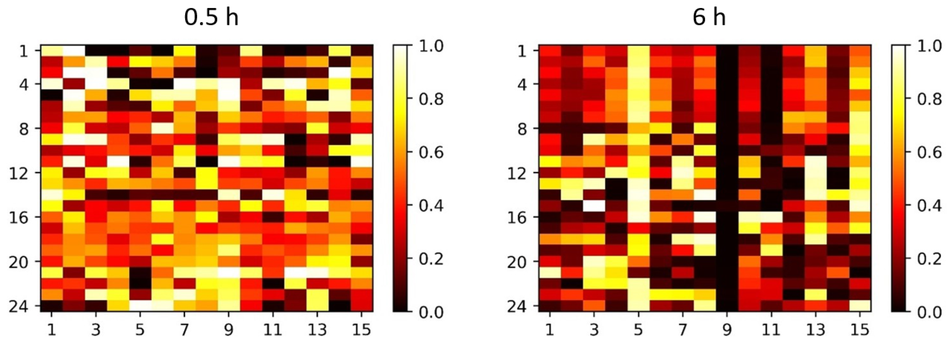
To further analyze the working mechanism of TSVEN, this paper visualizes the weight distribution of the GFM. For ease of explanation, the scenarios with time points 0.5 h and 6 h are taken as examples, and the results are shown in Figure 5. The number of hidden units in the LSTM is set to 15. According to Equation (9), the output of GFM is a 15-dimensional vector. For a given coordinate $x_k$, $y_n$—where $y_n$ ($1\le n\le 24$) denotes the n-th observation point—the x-axis represents the value of the k-th dimension ($1\le k\le 15$) of the GFM output vector. According to Equation (9), if $x_k=0$, TSVEN discards the semantic information of non-predictive variables in the k-th dimension, retaining only the semantic information of the target variable in this dimension; conversely, if this condition is not met, TSVEN does not retain the semantic information of chlorophyll concentration in the m-th dimension. As can be seen from Figure 5, GFM does not completely discard information from chlorophyll or non-predictive variables, but instead performs selective fusion of such information. This indicates that TSVEN effectively compresses harmful interactions between chlorophyll and non-predictive variables by dynamically balancing the information sources of its output items, thereby reducing the negative impact caused by information conflicts.

Effectiveness of DyAN To verify the effectiveness of DyAN, this paper also designed and evaluated two sets of comparative experiments: (i) DCAN vs. DCAN-Dv1, and (ii) DCAN-Dv2 vs. MTSMFF. Through the analysis of model structures, it can be known that compared with DCAN-Dv1 and MTSMFF, DCAN and DCAN-Dv2 have respectively introduced two key components of DyAN—the context attention mechanism and the FGM—on their basis. As shown in Table 3, the performance of DCAN is better than that of DCAN-Dv1, and this result further verifies the effectiveness of DyAN in improving the performance of chlorophyll concentration forecasting.

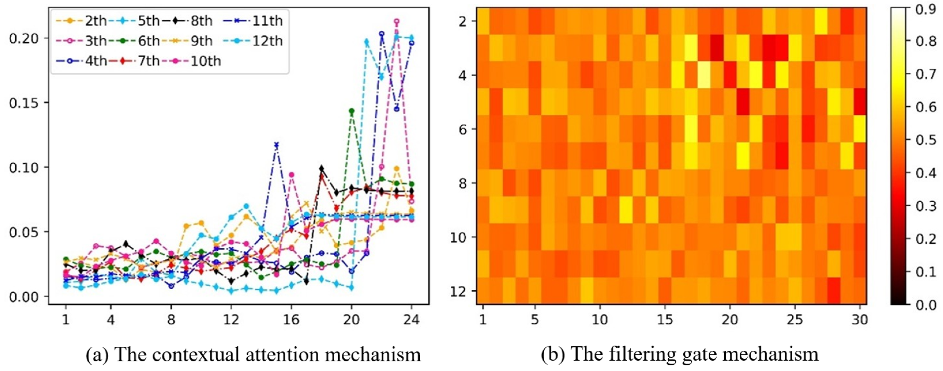
To further analyze the working mechanism of DyAN, Figure 6 shows the parameter distribution of the context attention mechanism and the filtering gate at the 6 h time point. In this experimental setup, the hidden unit size of the LSTM is set to 15. It should be noted that since the first forecasting time step does not involve the use of decoder hidden states, the visualization results only cover the 2-th to 12-th forecasting time steps. In Figure 6a, the abscissa represents the index of hidden states in the information queue focused on by the context attention. For the i-th ($2\le i\le 12$) curve, when the abscissa satisfies $k>(24-i+1)$, the corresponding $x_k$ is a decoder hidden state; otherwise, it is an encoder hidden state. The ordinate represents attention weights, where a larger weight indicates a higher importance of the hidden state $x_k$ for the current forecasting. In Figure 6b, the visualization results of the filtering gate outputs are presented. According to Equation (25), the output of the filtering gate is a 30-dimensional vector. For a given coordinate ($x_m,y_n$), $y_n$ denotes the context vector of the n-th ($2\le n\le 12$) forecasting point, and $x_m$ represents the value of the m-th ($1\le m\le 30$) dimension of the filtering gate output at this time step. As can be seen from Figure 6a, the hidden states with higher weights are mainly concentrated in the right region, indicating that hidden states closer to the forecasting time point contribute more to the model performance. Combined with Equation (21), for the i-th forecasting time step (the i-th curve), the context attention mechanism integrates several decoder hidden states prior to this time step into the information vector. Figure 6b shows that only a few points have filtering gate output values close to 0, indicating that the FGM does not completely discard the information of vector $y_n$, but selectively integrates it into the hidden state of the current decoder. Combining Equation (21) with the visualization results in Figure 6a, it can be judged that the filtering gate retains, to a certain extent, the information of the previous hidden states in the decoder unit. According to the experimental results shown in Table 3 and Figure 6, DCAN/DCAN-DV2 exhibit better forecasting performance than DCAN-DV1/MTSMFF. The reason lies in that the former has introduced more DyAN modules in their network structures. Therefore, based on the above analysis, it can be concluded that the hidden state information from the previous decoder unit provides effective auxiliary support for the current forecasting.

4.4.3. The Importance of Non-Predictive Variables

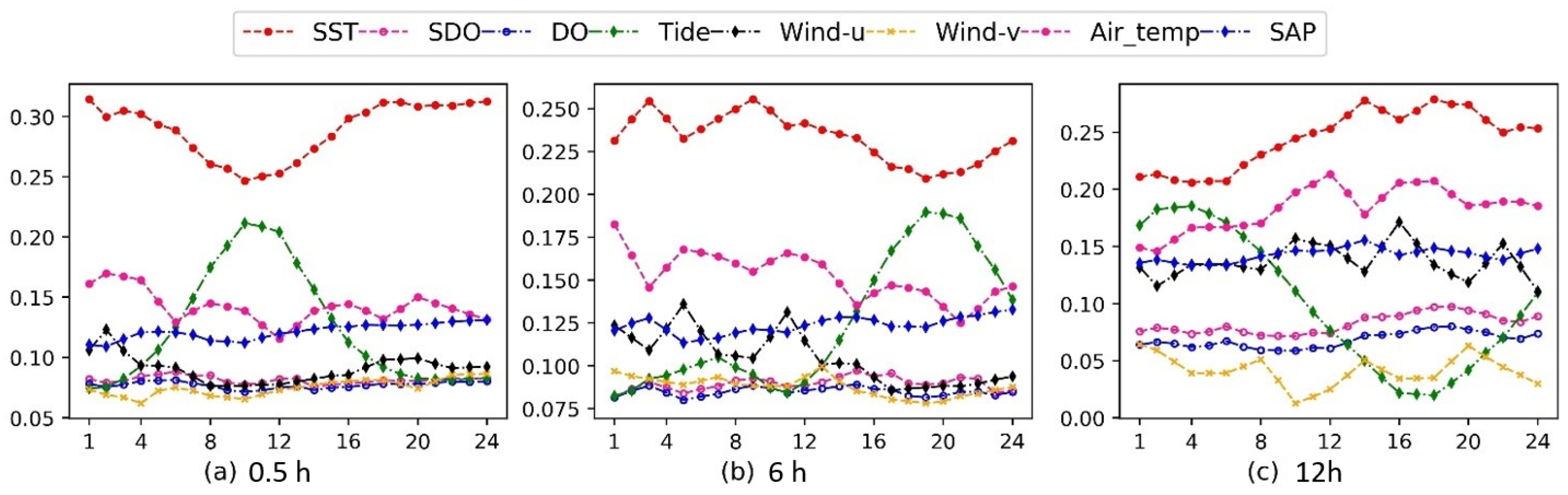
To further explore the role of non-predictive variables in the forecasting task, this section qualitatively analyzes the importance of each variable by visualizing the weight distribution of the VDN module. For ease of explanation, Figure 7 only presents the visualization results under the application scenarios with 0.5 h, 6 h, 12 h time points. In Figure 7, the x-axis represents each time step within the horizon, and the y-axis denotes the weight value obtained by the corresponding variable at that time point. A larger weight value indicates a more significant impact of the variable on the forecasting result. It can be intuitively seen from Figure 7 that within the given time range, different non-predictive variables have varying impacts on the chlorophyll sequence, and their importance changes over time. This shows that DCAN can not only effectively identify the importance of each variable but also capture their dynamic change trends. As shown in the evaluation results of Figure 7, SST and air temp have the highest weights in the forecasting, which is consistent with the conclusions of existing studies [31,32]. Therefore, the experimental results verify the effectiveness of the proposed DCAN model and indicate that it has a certain explanatory ability in forecasting tasks. In addition, the visualization results also show that the variable distillation attention mechanism can effectively reduce the interference of irrelevant variables on the forecasting results by assigning lower weights to them.

5. Discussion

Multistep-ahead chlorophyll concentration forecasting is critical for harmful algal bloom (HAB) early warning and coastal ecosystem management. This study proposed the Dynamic Collaborative Attention Network (DCAN) to address key challenges in this task, and the results offer valuable ecological and technical insights, aligned with existing research and constrained by the study’s scope.

The variable importance analysis (Figure 7) confirms that chlorophyll dynamics in Xiamen’s Eastern Water are driven by time-varying environmental factors. Sea surface temperature (SST), air temperature, tides, and dissolved oxygen (DO) emerged as key influencers—consistent with prior findings that temperature regulates phytoplankton growth [31,32] and tides affect coastal water exchange. Tidal weights were higher in short-horizon forecasts (reflecting immediate mixing effects), while SST maintained stable importance across time scales, reflecting cumulative thermal impacts on phytoplankton metabolism. This aligns with the observed correlation between chlorophyll diurnal fluctuations and tidal periodicity, validating the biological relevance of the selected variables.

DCAN’s superior performance over baselines (Table 1 and Table 2) stems from its modular design. The Temporal-Spatial Variable Enhancement Network (TSVEN) suppresses noise and redundant information, as evidenced by ablation results (Table 3) showing DCAN-Dv1 (TSVEN-only) outperforming MTSMFF. The Dynamic Attention Network (DyAN) mitigates error accumulation in multistep forecasting, with context attention and filtering gates (Figure 6) preserving prediction stability even at 48 h horizons—critical for extending HAB response windows. DCAN’s interpretability (Figure 5, Figure 6 and Figure 7) bridges data-driven modeling and ecological insight, as its attention mechanisms align with biological plausibility (e.g., dynamic variable weights) and corroborate existing research on temperature and hydrological drivers [33]. Ablation studies further confirm the synergistic role of TSVEN and DyAN in improving accuracy. Practically, DCAN’s accurate multistep forecasts support proactive coastal management (e.g., aquaculture adjustments). However, limitations remain: training on a single dataset restricts generalization, and higher computational complexity may hinder real-time deployment. Future work will focus on multi-dataset validation and model lightweighting, as noted in the conclusion.

In summary, DCAN advances chlorophyll forecasting by balancing performance and interpretability, grounded in ecological dynamics. Its findings reinforce the value of integrating attention mechanisms with ecological insight, providing a practical tool for HAB mitigation and coastal ecosystem management.

6. Conclusions

Due to the high complexity of the marine environment, multistep-ahead forecasting of chlorophyll is regarded as a challenging task. This paper proposes an attention mechanism-based forecasting framework—DCAN). The framework consists of a TSVEN and a DyAN. TSVEN utilizes a variable distillation attention mechanism to reduce the impact of irrelevant non-predictive variables and alleviates information conflicts between chlorophyll and non-predictive variables through a GFM. DyAN, on the other hand, mines the encoder outputs most relevant to forecasting via a temporal attention mechanism and realizes the interactive modeling between the encoder, previous decoder states, and current forecasting with the proposed context attention mechanism. Experimental results demonstrate that DCAN outperforms current mainstream advanced methods in forecasting performance. In addition, this paper conducts a visualization analysis of all attention layers in the model, further verifying the interpretability of the model. Meanwhile, the analysis results also indicate that the impacts of the chlorophyll target sequence and non-predictive variables on the forecasting task do not occur synchronously. Although the proposed Dynamic Collaborative Attention Network (DCAN) has achieved excellent performance, its generalization ability has not been fully verified due to being based solely on a single dataset. In the future, we plan to validate it using various different datasets. In addition, the computational complexity of DCAN is relatively high, and we are investigating how to lightweight it through techniques such as model pruning to improve operational efficiency.

References

1. Zhu, X.; Guo, H.; Huang, J.J.; Tian, S.; Zhang, Z. A hybrid decomposition and Machine learning model for forecasting Chlorophyll-a and total nitrogen concentration in coastal waters. J. Hydrol. 2023, 619, 129207. [Google Scholar] [CrossRef] [Scilit]
2. Liu, N.; Chen, S.; Cheng, Z.; Wang, X.; Xiao, Y.; Xiao, L.; Gong, Y.; Wang, T.; Zhang, X.; Liu, S. Long-term prediction of sea surface chlorophyll-a concentration based on the combination of spatio-temporal features. Water Res. 2022, 211, 118040. [Google Scholar] [CrossRef] [Scilit]
3. Mu, B.; Qin, B.; Yuan, S.; Wang, X.; Chen, Y. PIRT: A Physics-Informed Red Tide Deep Learning Forecast Model Considering Causal-Inferred Predictors Selection. IEEE Geosci. Remote Sens. Lett. 2023, 20, 1–5. [Google Scholar] [CrossRef] [Scilit]
4. Peng, S.; Yu, X.; Lee, Z.; Lin, H.; Liu, X.; Dai, M.; Shang, S. Ocean’s largest chlorophyll-rich tongue is extending westward (2002–2022). Nat. Commun. 2025, 16, 103. [Google Scholar] [CrossRef] [Scilit]
5. Jia, W.; Cheng, J.; Hu, H. A Cluster-Stacking-Based Approach to Forecasting Seasonal Chlorophyll-a Concentration in Coastal Waters. IEEE Access 2020, 8, 99934–99947. [Google Scholar] [CrossRef] [Scilit]
6. Ham, Y.G.; Joo, Y.S.; Park, J.Y. Mechanism of skillful seasonal surface chlorophyll prediction over the southern Pacific using a global earth system model. Clim. Dyn. 2021, 56, 45–64. [Google Scholar] [CrossRef] [Scilit]
7. Barzegar, R.; Aalami, M.; Adamowski, J. Short-term water quality variable prediction using a hybrid CNN–LSTM deep learning model. Stoch. Environ. Res. Risk Assess. 2020, 34, 415–433. [Google Scholar] [CrossRef] [Scilit]
8. Chang, W.; Li, X.; Chaudhary, V.; Dong, H.; Zhao, Z.; Nguyen, T.G. Prediction of chlorophyll-a data based on triple-stage attention recurrent neural network. IET Commun. 2025, 19, e12542. [Google Scholar] [CrossRef] [Scilit]
9. Wu, S.S.; Du, Z.H.; Zhang, F.; Zhou, Y.; Liu, R.Y. Time-Series Forecasting of Chlorophyll-a in Coastal Areas Using LSTM, GRU and Attention-Based RNN Models. J. Environ. Inform. 2023, 41, 104. [Google Scholar] [CrossRef] [Scilit]
10. Ye, H.; Tang, S.; Yang, C.; Chen, C. Reconstruction of Daily MODIS/Aqua Chlorophyll-a Concentration in Turbid Estuarine Waters Based on Attention U-NET. Remote Sens. 2023, 15, 546. [Google Scholar] [CrossRef] [Scilit]
11. Li, H.; Shen, Y.; Zhu, Y. Stock Price Prediction Using Attention-based Multi-Input LSTM. In PMLR, Proceedings of the 10th Asian Conference on Machine Learning, Beijing, China, 14–16 November 2018; Zhu, J., Takeuchi, I., Eds.; Proceedings of Machine Learning Research: Stockholm, Sweden, 2018; Volume 95, pp. 454–469. [Google Scholar]
12. Muralidhar, N.; Muthiah, S.; Ramakrishnan, N. DyAt Nets: Dynamic Attention Networks for State Forecasting in Cyber-Physical Systems. In Proceedings of the Twenty-Eighth International Joint Conference on Artificial Intelligence, Macao, China, 10–16 August 2019; pp. 3180–3186. [Google Scholar] [CrossRef] [Scilit]
13. Cui, Q.; Wu, S.; Huang, Y.; Wang, L. A hierarchical contextual attention-based network for sequential recommendation. Neurocomputing 2019, 358, 141–149. [Google Scholar] [CrossRef] [Scilit]
14. Papenfus, M.; Schaeffer, B.; Pollard, A.; Loftin, K. Exploring the potential value of satellite remote sensing to monitor chlorophyll-a for US lakes and reservoirs. Environ. Monit. Assess. 2020, 192, 808. [Google Scholar] [CrossRef] [Scilit]
15. Jin, S.H.; Jargal, N.; Khaing, T.T.; Cho, M.J.; Choi, H.; Ariunbold, B.; Donat, M.G.; Yoo, H.; Mamun, M.; An, K.G. Long-term prediction of algal chlorophyll based on empirical models and the machine learning approach in relation to trophic variation in Juam Reservoir, Korea. Heliyon 2024, 10, e31643. [Google Scholar] [CrossRef] [Scilit] [PubMed]
16. Hadjal, M.; Medina-Lopez, E.; Ren, J.; Gallego, A.; McKee, D. An Artificial Neural Network Algorithm to Retrieve Chlorophyll a for Northwest European Shelf Seas from Top of Atmosphere Ocean Colour Reflectance. Remote Sens. 2022, 14, 3353. [Google Scholar] [CrossRef] [Scilit]
17. Kim, D.; Lee, K.; Jeong, S.; Song, M.; Kim, B.; Park, J.; Heo, T.Y. Real-time chlorophyll-a forecasting using machine learning framework with dimension reduction and hyperspectral data. Environ. Res. 2024, 262, 119823. [Google Scholar] [CrossRef] [Scilit]
18. Pahlevan, N.; Smith, B.; Schalles, J.; Binding, C.; Cao, Z.; Ma, R.; Alikas, K.; Kangro, K.; Gurlin, D.; Hà, N.; et al. Seamless retrievals of chlorophyll-a from Sentinel-2 (MSI) and Sentinel-3 (OLCI) in inland and coastal waters: A machine-learning approach. Remote Sens. Environ. 2020, 240, 111604. [Google Scholar] [CrossRef] [Scilit]
19. Bui, H.; Pham, T.L.; Dao, S. Prediction of cyanobacterial blooms in the Dau Tieng Reservoir using an artificial neural network. Mar. Freshw. Res. 2017, 68, 2070–2080. [Google Scholar] [CrossRef] [Scilit]
20. Cen, H.; Jiang, J.; Han, G.; Lin, X.; Liu, Y.; Jia, X.; Ji, Q.; Li, B. Applying Deep Learning in the Prediction of Chlorophyll-a in the East China Sea. Remote Sens. 2022, 14, 5461. [Google Scholar] [CrossRef] [Scilit]
21. Yao, L.; Wang, X.; Zhang, J.; Yu, X.; Zhang, S.; Li, Q. Prediction of Sea Surface Chlorophyll-a Concentrations Based on Deep Learning and Time-Series Remote Sensing Data. Remote Sens. 2023, 15, 4486. [Google Scholar] [CrossRef] [Scilit]
22. Mohamed Yussof, F.; Maan, N.; Md Reba, M.N. LSTM Networks to Improve the Prediction of Harmful Algal Blooms in the West Coast of Sabah. Int. J. Environ. Res. Public Health 2021, 18, 7650. [Google Scholar] [CrossRef] [Scilit]
23. Nurhamidah, N.; Nusyirwan, N.; Faisol, A. Forecasting Seasonal Time Series Data using The Holt-Winters Exponential Smoothing Method of Additive Models. J. Mat. Integr. 2020, 16, 151–157. [Google Scholar] [CrossRef] [Scilit]
24. Ning, Y.; Kazemi, H.; Tahmasebi, P. A comparative machine learning study for time series oil production forecasting: ARIMA, LSTM, and Prophet. Comput. Geosci. 2022, 164, 105126. [Google Scholar] [CrossRef] [Scilit]
25. Wan, R.; Mei, S.; Wang, J.; Liu, M.; Yang, F. Multivariate Temporal Convolutional Network: A Deep Neural Networks Approach for Multivariate Time Series Forecasting. Electronics 2019, 8, 876. [Google Scholar] [CrossRef] [Scilit]
26. Hu, J.; Zheng, W. Multistage attention network for multivariate time series prediction. Neurocomputing 2020, 383, 122–137. [Google Scholar] [CrossRef] [Scilit]
27. Du, S.; Li, T.; Yang, Y.; Horng, S.J. Multivariate time series forecasting via attention-based encoder–decoder framework. Neurocomputing 2020, 388, 269–279. [Google Scholar] [CrossRef] [Scilit]
28. Shih, S.Y.; Sun, F.K.; Lee, H.y. Temporal pattern attention for multivariate time series forecasting. Mach. Learn. 2019, 108, 1421–1441. [Google Scholar] [CrossRef] [Scilit]
29. Liu, Y.; Gong, C.; Yang, L.; Chen, Y. DSTP-RNN: A dual-stage two-phase attention-based recurrent neural network for long-term and multivariate time series prediction. Expert Syst. Appl. 2020, 143, 113082. [Google Scholar] [CrossRef] [Scilit]
30. Kingma, D.P.; Ba, J. Adam: A Method for Stochastic Optimization. arXiv 2014, arXiv:1412.6980. [Google Scholar]
31. Liu, X.; Feng, J.; Wang, Y. Chlorophyll a predictability and relative importance of factors governing lake phytoplankton at different timescales. Sci. Total Environ. 2019, 648, 472–480. [Google Scholar] [CrossRef] [Scilit] [PubMed]
32. Cha, Y.; Cho, K.H.; Lee, H.; Kang, T.; Kim, J.H. The relative importance of water temperature and residence time in predicting cyanobacteria abundance in regulated rivers. Water Res. 2017, 124, 11–19. [Google Scholar] [CrossRef] [Scilit]
33. Wallace, J.; Champagne, P.; Hall, G. Time series relationships between chlorophyll-a, dissolved oxygen, and pH in three facultative wastewater stabilization ponds. Environ. Sci. Water Res. Technol. 2016, 2, 1032–1040. [Google Scholar] [CrossRef] [Scilit]
Figure 1. Overall workflow of dynamic collaborative attention network.
Jmse 13 02353 g001
Figure 2. Visualization of performance for different methods.
Jmse 13 02353 g002
Figure 3. Prediction results of DA-TLSTM, DCAN, and DSTP-RNN versus the ground truth at the 2nd h (with fitted curves).
Jmse 13 02353 g003
Figure 4. Prediction results of DA-TLSTM, DCAN, and DSTP-RNN versus the ground truth at the 48th h.
Jmse 13 02353 g004
Figure 5. Visualization display of the performance of the gated fusion module.
Jmse 13 02353 g005
Figure 6. Visualization of the contextual attention mechanism and filtering gate mechanism at th 6 h time point.
Jmse 13 02353 g006
Figure 7. The importance levels of different non-predictive variables.
Jmse 13 02353 g007