Article

Long-Term Trends, Interannual Variability and Seasonal Patterns of Mean Sea Level in the Canary Islands

by
Mikel Ibeas
* and
Antonio Martínez-Marrero
Instituto de Oceanografía y Cambio Global (IOCAG), Universidad de Las Palmas de Gran Canaria (ULPGC), 35017 Las Palmas de Gran Canaria, Spain
*
Author to whom correspondence should be addressed.
J. Mar. Sci. Eng. 2025, 13(11), 2193; https://doi.org/10.3390/jmse13112193
Submission received: 1 October 2025 / Revised: 1 November 2025 / Accepted: 12 November 2025 / Published: 18 November 2025

Abstract

This study analyzes mean sea level variability in the Canary Islands from 1993 to 2022 using tide gauge and satellite altimetry data. During this period, both Las Palmas de Gran Canaria and Santa Cruz de Tenerife exhibited a significant sea level rise of 4.04 ± 0.83 and 4.38 ± 0.93 mm yr−1, respectively. Comparison between tide gauge and altimetry records reveals slight land subsidence at both locations, approximately 0.5–0.7 ± 0.55 mm yr−1, contributing to the observed relative sea level rise. The spatial differences in the trends observed from altimetry appear to be associated with mesoscale ocean dynamics, particularly an increase in eddy activity along the Canary Eddy Corridor. Projections based on IPCC SSP scenarios suggest that sea level could rise by up to 395 mm in Santa Cruz and 365 mm in Las Palmas by 2050 under high-emission conditions. An additional 20 mm could be added due to land subsidence if it remains constant. Interannual variability is primarily correlated with the North Atlantic Oscillation (NAO); however, Atlantic Multidecadal Oscillation (AMO) and the Atlantic Meridional Overturning Circulation (AMOC) indices also appear to correlate well with its low-frequency components. The seasonal cycle, driven primarily by steric effects, peaks in late summer and reaches a minimum in late winter, with its amplitude varying across the region. The seasonal amplitude is approximately 49.6 mm in Las Palmas and 70.2 mm in Santa Cruz.

1. Introduction

Changes in mean sea level are associated with some of the most severe impacts of climate change, including flooding, coastal erosion, saline intrusion, ecosystem loss, and an increased risk to infrastructure and services [1]. The global rise in sea levels has accelerated significantly over recent decades, driven primarily by thermal expansion of seawater and melting ice from glaciers and polar ice sheets. In Europe, it is estimated that more than 50 million people live in areas below 10 m in altitude, making them particularly vulnerable to these variations [2]. Therefore, sea level is a variable of great relevance both for scientific research and for land use planning and public policy formulation.
Global mean sea level (GMSL) estimates are key indicators of ongoing global warming, but changes in regional sea level prove more relevant for local risk management [3,4,5,6]. Regional or local mean sea level (LMSL) observations demonstrate significant spatial and temporal variability, posing a challenge for planning adaptation measures.
The Canary Islands are an example of a region that is particularly vulnerable to sea level rise because of their oceanic island characteristics. According to the IPCC Special Report, “Sea Level Rise and Implications for Low-Lying Islands, Coasts, and Communities” [7], island regions and archipelagos, are at a heightened risk due to their limited adaptative capacities, high concentrations of coastal infrastructures, and exposure to extreme wave and storm events. Despite these vulnerabilities, comprehensive studies focusing on sea level reconstructions and future projections for the Canary Islands specifically remain scarce [8,9].
Analyzing sea level variability requires studying the three main temporal scales commonly used in oceanographic research: long-term trends, interannual fluctuations, and seasonal cycles [10,11]. These scales capture different driving mechanisms and are critical for understanding both the background rise in sea level and its shorter-term variability. The following sections briefly describe each of these components:
  • Long-term trends
Most available data show a continuous rise in GMSL since the early 20th century, with a notable acceleration in recent decades [12]. A significant number of authors have generated reconstructions of GMSL from tide gauge records [13,14,15]. The most recent study, by Frederikse et al. [12], estimated a GMSL rise of 1.56 ± 0.33 mm yr−1 between 1900 and 2018. However, since 1993, this rate has accelerated, reaching 3.35 ± 0.4 mm yr−1, consistent with altimetric data [16].
The contributions of various drivers have been quantified through parameterizations and process-based models. These estimates suggest that approximately 50% of the observed global sea level rise is due to thermal expansion, while the remaining 50% is mainly attributed to glacier melt, the loss of ice from Greenland and Antarctica, and groundwater depletion [12,17].
Long-term sea level changes exhibit a pronounced regional component, making it essential to distinguish between global and local changes [18]. While GMSL largely reflects global-scale processes such as thermal expansion and continental ice loss [19], local sea level is also affected by a combination of other factors [7,20,21,22], including regional ocean dynamics (winds, currents, Kelvin and Rossby waves), uneven distribution of ocean warming, geographic patterns of ice melt and vertical land motion.
  • Interannual variability
In addition to long-term trends, mean sea level exhibits interannual variability driven by processes operating over several years. Major contributing factors include climate modes such as the El Niño–Southern Oscillation (ENSO), which can cause sea level fluctuations of several centimeters at regional and global scales [23]. Other phenomena, such as the North Atlantic Oscillation (NAO) and the Pacific Decadal Oscillation (PDO), also modulate sea level interannually, particularly in the North Atlantic and North Pacific [24,25]. On smaller spatial scales, mesoscale eddies can produce short-term fluctuations that also affect interannual variability as well [26,27].
  • Seasonal variability
Sea level exhibits marked temporal variability on seasonal time scales. This seasonal signal is primarily driven by the thermal expansion of seawater during warmer months and its contraction during colder months, resulting in an annual cycle of sea level rise and fall [26]. In addition to this steric component, seasonal storage of water in the form of snow and ice, particularly in the Northern Hemisphere during winter, temporarily reduces ocean volume [28]. This process, combined with seasonal wind stress and other atmospheric forcings, significantly modulates sea level at regional scales [29]. The combination of these factors can produce seasonal oscillations of mean sea level of several centimeters, with amplitudes that vary depending on geographic region and latitude [30].
Considering the background discussed above, this study aims to address the lack of specific research and monitoring by conducting an in-depth analysis of the mean sea level variations in the Canary Islands region from 1993 to 2022. The analysis will examine the temporal and spatial variability in sea level using tide gauge records and satellite altimetry data. The results seek to enhance understanding of local sea level dynamics and provide more accurate projections for adaptation and policy development.

2. Materials and Methods

2.1. Data

Four datasets were used in this study:
Monthly mean sea level records from the tide gauges at Las Palmas de Gran Canaria (LP) and Santa Cruz de Tenerife (SC), shown in Figure 1, covering the period from January 1993 to January 2023, were obtained from the Permanent Service for Mean Sea Level global repository (PSMSL, https://psmsl.org/data/, accesed on 28 April 2025) [31,32]. These two stations were selected due to the length and completeness of their time series, which ensures the robustness of sea level trend estimation. Data from PSMSL was preferred because it undergo a rigorous quality control process that enhances reliability, particularly important when merging time series recorded with different types of instruments, as often occurs when equipment is updated or replaced. Among the PSMSL stations in the Canary Islands, only Las Palmas and Santa Cruz provide long, continuous, RLR-referenced monthly records spanning the full altimetric era. Other stations are shorter and/or discontinuous, which limits their utility for robust long-term trend estimation. We therefore use these two gauges to quantify local relative sea-level (RSL) change at port settings, and we complement them with the CMEMS gridded Level 4 altimetry to assess the archipelago-scale variability and trends.
From 1993 to 2009, both the Las Palmas and Santa Cruz tide-gauge stations operated with SRD acoustic sensors. In 2009 a one-year overlap was established to compare the SRD with the new MIROS radar sensors and determine any possible bias, ensuring continuity of the long-term sea-level record [33]. SRD sensors provide typical accuracy of ±1 cm (vertical resolution ~1 cm), suitable for operational port measurements, whereas MIROS radar sensors offer higher precision, with typical accuracy for averaged measurements ≲ ±5 mm. These practices follow IOC/GLOSS recommendations [34].
Monthly sea surface height above the ellipsoid derived from satellite altimeter for the Canary Islands region was obtained from the Global Ocean Gridded L4 Sea Surface Heights and Derived Variables–Reprocessed dataset provided by the Copernicus Marine Environment Monitoring Service (CMEMS) [35]. This Level 4 dataset merges and cross-calibrates multiple along-track missions into a 0.25° × 0.25° grid (1993–2024). We extracted the nearest grid cell to each tide gauge and computed monthly means. Product accuracy and homogeneity are documented in the CMEMS Quality Information Document (QUID). Independent assessments indicate that Data Unification and Altimeter Combination System (DUACS) maps resolve wavelengths of ~100–300 km (mid-latitudes) with an effective temporal resolution close to monthly [36]. Thus, while the gridded fields are well suited to analyzing regional variability and trends, they cannot fully resolve very local coastal signals that a point tide gauge may record.
For each tide gauge we extracted the nearest open-ocean grid cell and computed monthly means on the same calendar (Figure 1). Consistent with previous work, altimetric series near gauges generally agree well at monthly and longer time scales over oceanic islands [37], whereas agreement can be poorer along continental coasts where local processes and land-proximity effects are stronger [29].
Sea surface temperature (SST) for the study area was obtained from the Multi-Observation Global Ocean ARMOR3D L4 analysis and multi-year reprocessed product provided by the CMEMS. The dataset covers the period 1993–2023 and includes monthly fields of temperature, salinity, sea level, geostrophic currents, and mixed layer depth, all provided on a regular 1/8° grid.
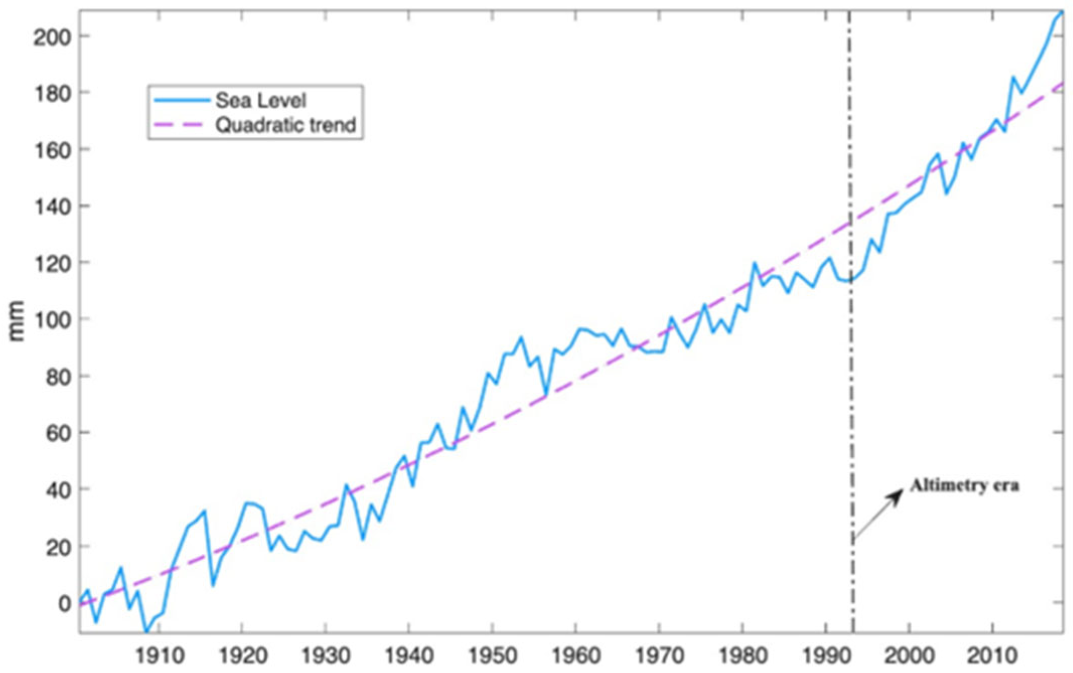
Monthly time series of GMSL variation from 1900 to 2018 were obtained from the reconstruction developed by Frederikse et al. (available at https://zenodo.org/records/6067895, accessed on 17 March 2025) [12]. This model combines observations of ocean mass (barystatic component) and thermal expansion (thermosteric component), along with tide gauge records from around the globe corrected for vertical land motion and gravitational effects. The resulting dataset is illustrated in Figure 2.
In addition, complementary information was obtained for comparison with other sources:
Vertical land motion data derived from GNSS measurements were obtained from the PSMSL and the Système d’Observation du Niveau des Eaux Littorales (SONEL). These data are available at https://psmsl.org (accessed on 28 April 2025) and https://www.sonel.org (accessed on 22 April 2025). The results of two recent studies by Barbero et al. [38] and Pfeffer & Allemand [22] were also used.
Sea level rise projections produced by NASA for the most recent Assessment Report of the Intergovernmental Panel on Climate Change [1]. These projections, based on historical reconstructions and coupled ocean–cryosphere model simulations, provide estimates of future sea level changes through the year 2150. They are accessible via an interactive tool at https://sealevel.nasa.gov/ipcc-ar6-sea-level-projection-tool (accessed on 22 April 2025) [39].

2.2. Methodology

All-time series processing, statistical analyses, visualizations, and spectral evaluations were performed within the MATLAB R2024b environment.
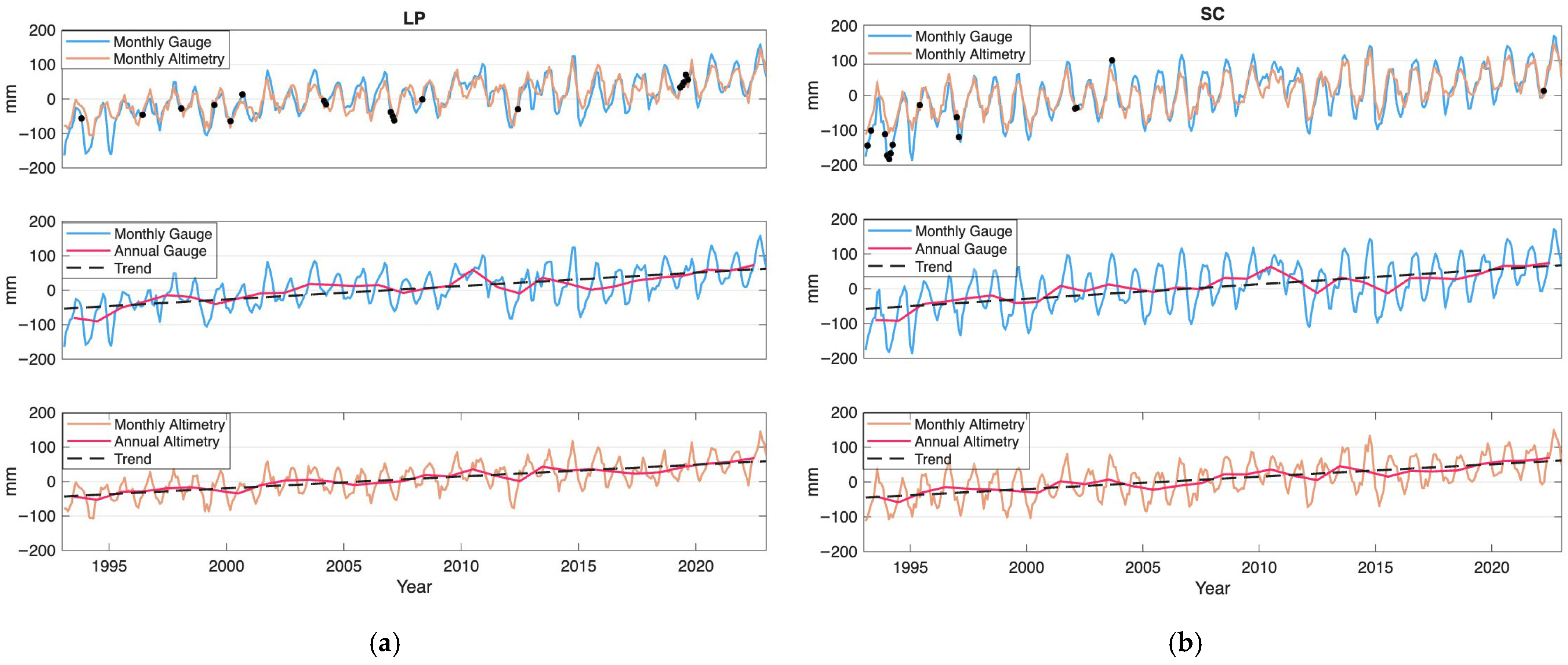
First, the monthly time series from the tide gauges and the satellite altimetry were examined and harmonized in length to allow for direct comparison. As shown in Figure 3, the tide gauge records contain some data gaps. Overall, the data coverage is good, with no more than two consecutive missing months, except at the LP station, which has four consecutive missing months between the end of 2018 and the beginning of 2019. These missing values were linearly interpolated at the same time steps as the satellite altimetry data to facilitate a consistent comparison of the two datasets.
The inverted barometer effect (i.e., sea level variations caused by the hydrostatic response of the ocean to changes in atmospheric pressure) was not removed from the tide gauge records. This reflects the study’s focus on analyzing effective sea level variability rather than isolating individual forcing mechanisms.
Linear trends were estimated using generalized least squares (GLS) with an AR(1) stochastic–noise model for the residuals, in line with best practice for geophysical time-series analysis [40,41]. For the monthly series we fitted an intercept and a linear trend, included a seasonal component (annual cycle), and tested for possible step changes (offsets). Uncertainties are reported as 95% confidence intervals (CIs) from the GLS covariance; statistical significance was assessed by the two-sided test on the trend parameter (equivalently, by checking whether the 95% CI excludes zero). As robustness checks, we repeated the analysis using annual means (which reduces seasonal distortion) and computed ordinary least squares with Newey–West (heteroskedasticity and autocorrelation consistent) standard errors; all approaches yielded consistent trend estimates.
To investigate sea level variability across different temporal scales, standard procedures recommended by Pugh and Woodworth [10] were applied:
  • Trend estimation: Obtained by fitting a GLS model with AR(1) residuals to the monthly time series, as described above. To avoid biases due to incomplete seasonal cycles, years with missing months at the beginning or end of the series were excluded from the analysis.
  • Interannual anomalies: Obtained by subtracting the long-term linear trend from the annual mean sea level values.
  • Seasonal anomalies: Obtained by subtracting the annual mean sea level from the monthly mean sea level values.
Finally, spectral analysis was conducted using Welch’s method to identify dominant frequencies and characterize interannual variability. The MATLAB R2024b function pwelch was used for this purpose, applying a Hamming window to minimize spectral leakage and improve frequency resolution.

3. Results

3.1. Long-Term Variability

Figure 3 illustrates the variation in the monthly mean sea level recorded by the LP and SC tide gauges from 1993 to 2022 referenced to the mean sea level for the period 1995–2014, as the IPCC states in its latest Assessment Report [1]. It also shows the corresponding time series derived from satellite altimetry for nearby grid cells. There is clear agreement between the tide gauge and altimetry records. The figure also shows the annual mean sea level, revealing that although the mean sea level is rising overall, the increase is not monotonic. Specifically, the rate of sea level rise slowed from approximately 2000 to 2015, then accelerated again from 2015 to 2022.
Table 1 reports the GLS trends with 95% confidence intervals (CIs) and, in parentheses, the estimated AR(1) coefficient (ϕ) as a measure of residual persistence. As robustness checks, we repeated the analysis using annual means, which yielded consistent trends n. Tide-gauge records exhibit stronger residual persistence (larger ϕ) than the collocated gridded altimetry, as expected because harbour series contain locally forced variability (wind setup and inverse-barometer/meteorological effects) that is less visible in spatially averaged altimetry, and because the CMEMS Level-4 product maps and smooths small-scale coastal signals. This behaviour is consistent with published assessments of tide gauge–altimetry differences near coasts and with the documented effective resolution/smoothing of DUACS mapping [29]. Trends obtained by subtracting the tide gauge series from the altimetry series were used as a proxy for vertical land motion. At LP, the difference is not statistically distinguishable from zero at the 95% CI. At SC, however, the difference is weakly positive, with a CI that narrowly excludes zero. These results suggest small subsidence of approximately 0.5 mm per year in both locations from 1993 to 2022.
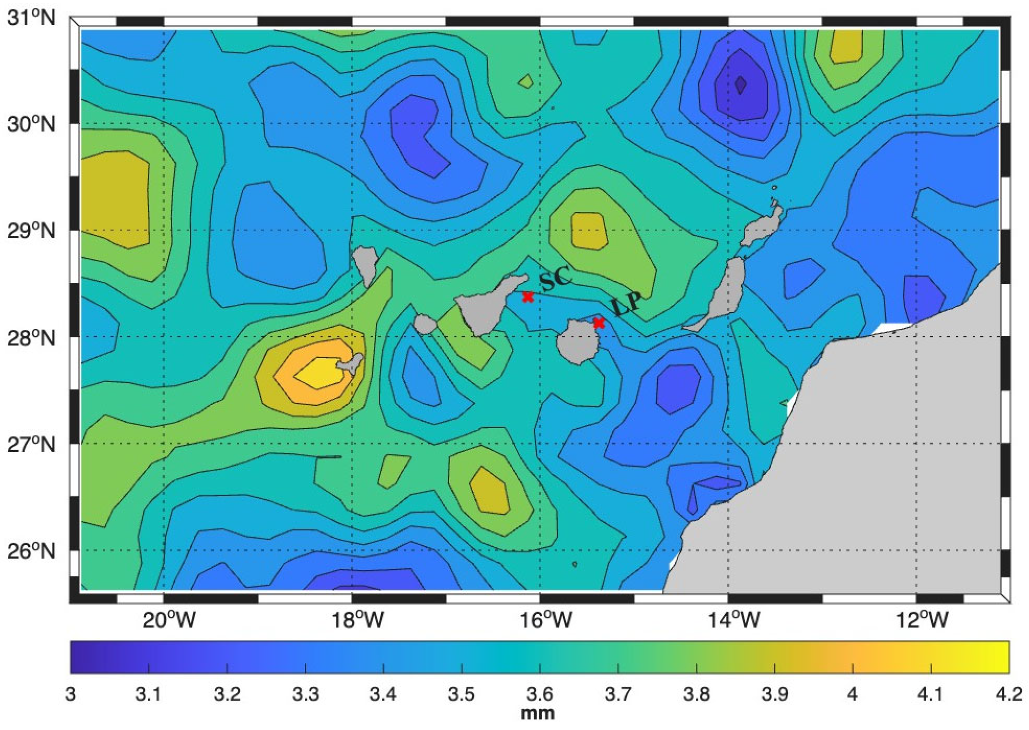
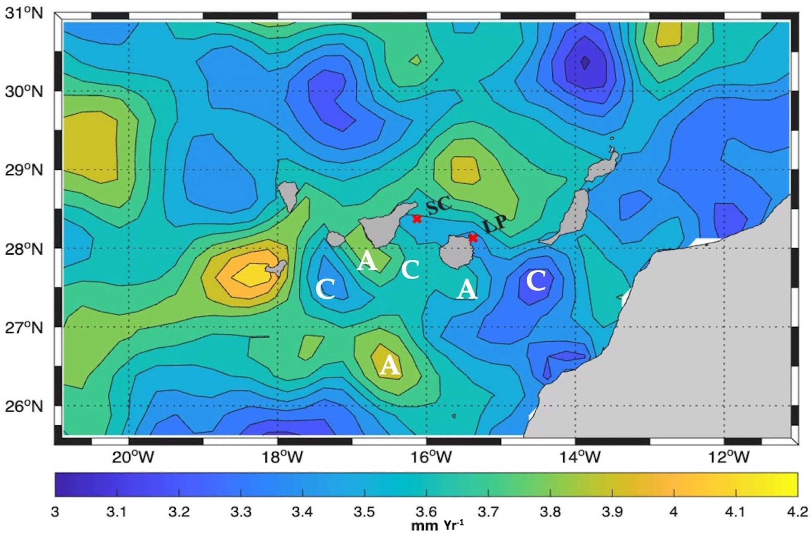
The mean sea level trend was calculated for each grid cell in the altimetric dataset (Figure 4). The results reveal complex spatial variability in sea level rise at the scale of typical mesoscale phenomena (~100 km), with values ranging from 3 to 4 mm yr−1.

3.2. Interannual Anomalies

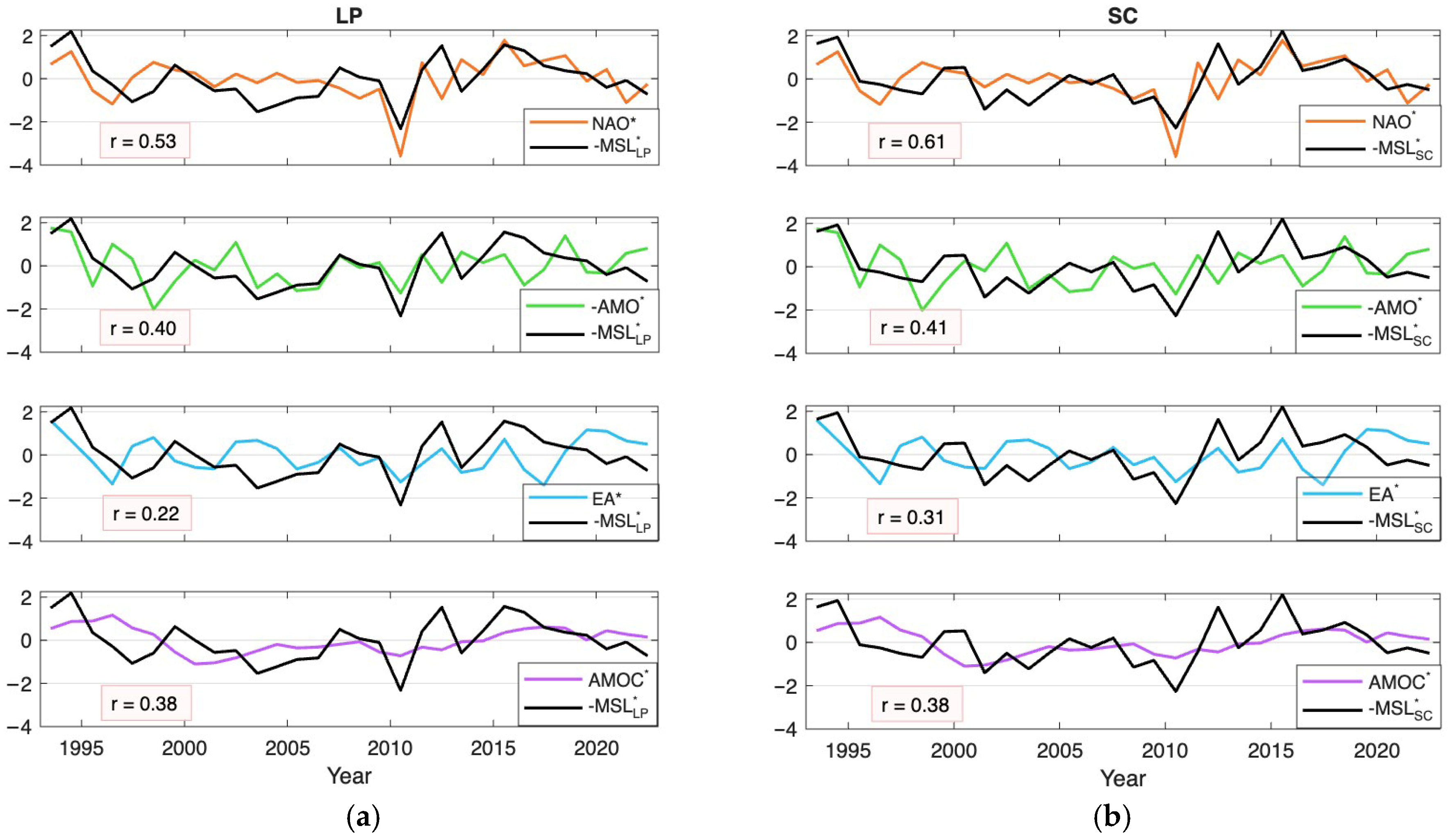
The interannual sea level anomaly was calculated by removing the linear trend from the annual mean sea level time series [10]. The resulting anomaly was then normalized by dividing the residuals by their standard deviation. Figure 5 displays this normalized anomaly and compares it with four climate indices (each also detrended to focus on interannual variability): (a) the NAO index, which quantifies the difference in normalized sea-level pressure between the subtropical high-pressure system near the Azores and the subpolar low near Iceland; (b) the Atlantic Multidecadal Oscillation (AMO) index, derived from spatially averaged North Atlantic SST anomalies (typically 0–60° N) after removing the global mean SST signal, represents natural multidecadal variations between warm and cool phases. (c) the East Atlantic (EA) pattern, defined as the second principal component of 500 hPa geopotential height anomalies over the North Atlantic, and (d) the Atlantic Meridional Overturning Circulation (AMOC), which quantifies the maximum value of vertically integrated meridional volume transport at 26.5° N.
Although some relationship can be observed between sea level at the LP and SC tide gauges and the four climate indices, the strongest correlation is found with the NAO (0.53 for LP and 0.61 for SC). In the case of the AMO and AMOC, however, its evolution resembles only the low-frequency variation in sea level and not the higher-frequency or rapid oscillations.

3.3. Seasonal Anomalies

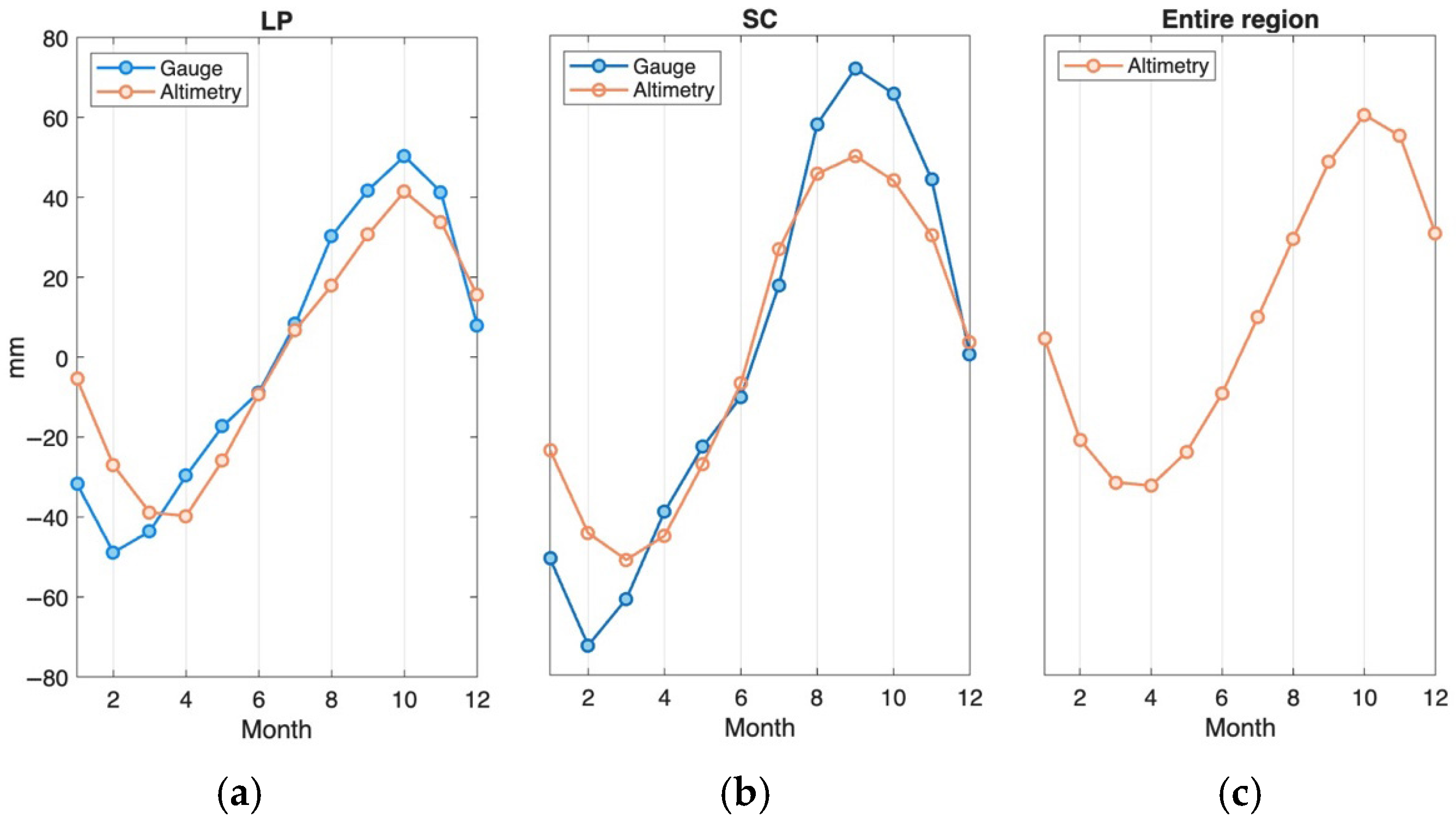
To calculate the seasonal sea level anomaly, the annual mean sea level was subtracted from each monthly value within the corresponding year [10]. The resulting anomalies were then averaged over the entire study period (1993–2022) for each calendar month, yielding a mean seasonal cycle. The results at both LP and SC stations, derived from tide gauge records and satellite altimetry in the study area (Figure 6), exhibit a consistent pattern: sea level typically reaches its annual maximum between September and October and its minimum between February and April. The signal from satellite altimetry exhibits a lower seasonal range (81.14 mm for LP and 101.02 mm for SC), compared with the tide gauge data (99.15 mm for LP and 144.40 mm for SC) likely due to the spatial smoothing applied in the reanalysis product which tends to attenuate local variability.
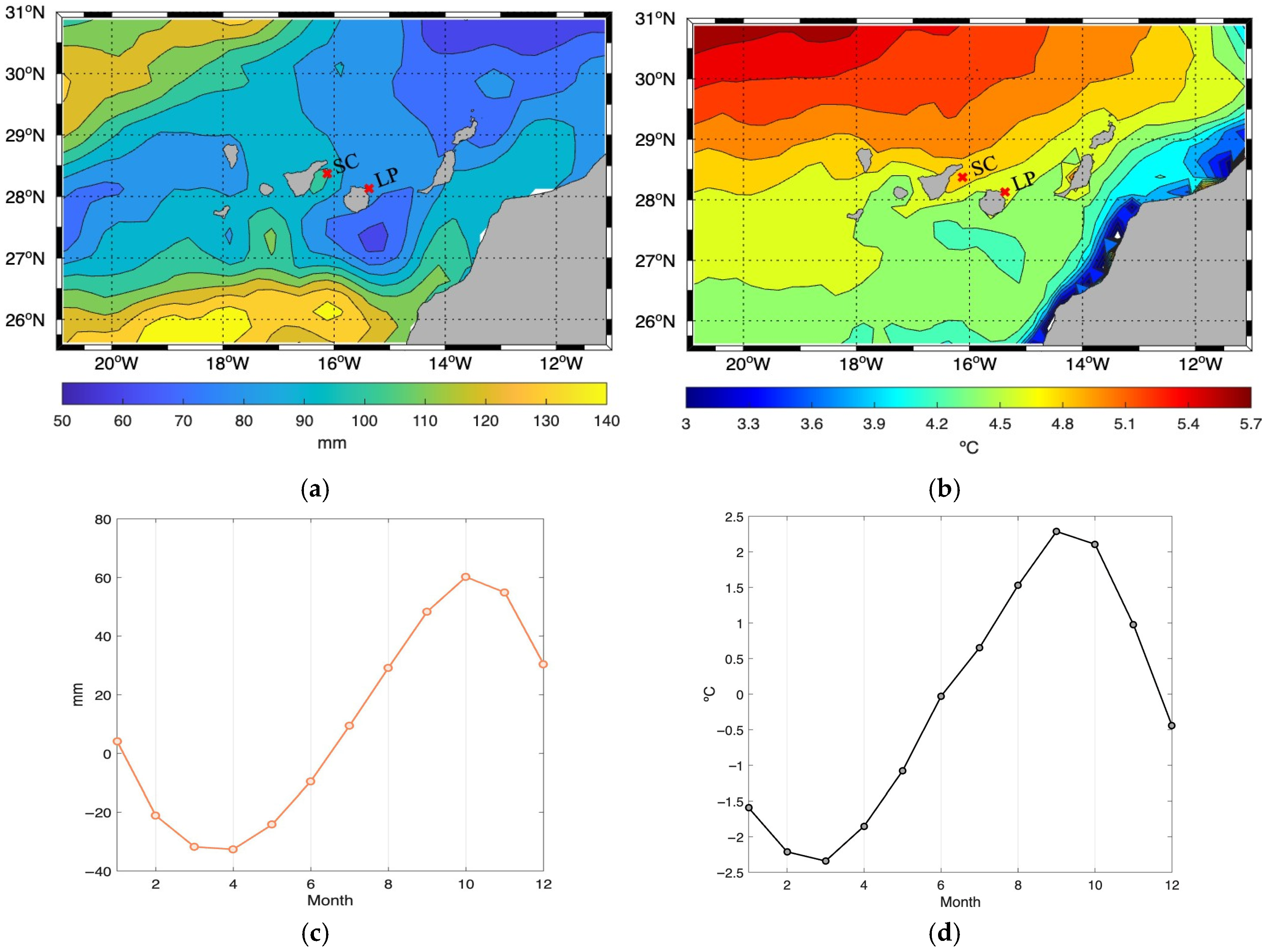
The same procedure was applied to the spatially averaged sea surface temperature dataset for the Canary region, obtained from the Multi-Observation Global Ocean ARMOR3D L4 Copernicus product (see Data section). The results (Figure 7d) evidence that the observed seasonal cycle is primarily driven by steric effects as sea surface temperatures peak in late summer and early autumn. In contrast, cooler temperatures in late winter and early spring reduce thermal expansion, resulting in lower sea levels. Additional contributions from seasonal wind stress and atmospheric pressure variability may further modulate coastal sea level on monthly timescales [11] and could account for the small differences observed between the two stations.
Figure 7a shows range of the seasonal oscillation (defined as the difference between the maximum and minimum values of the mean seasonal cycle) across the study area. This reveals significant spatial variability. A band of minimum height, ranging from approximately 60 to 80 mm, extends from around 27–28° N on the western edge of the domain towards the northeast. This band is flanked by two regions of maximum height: one to the south, where values reach 140 mm near 26° N, and another to the northwest, where values are around 120 mm.
When considering the seasonal oscillation of SST (Figure 7b), the spatial pattern does not fully align with the sea level pattern despite the temporal evolution of the seasonal cycles are very similar (see Figure 7c,d). These results suggest that additional local factors may influence the spatial variability of the seasonal cycle in this region.
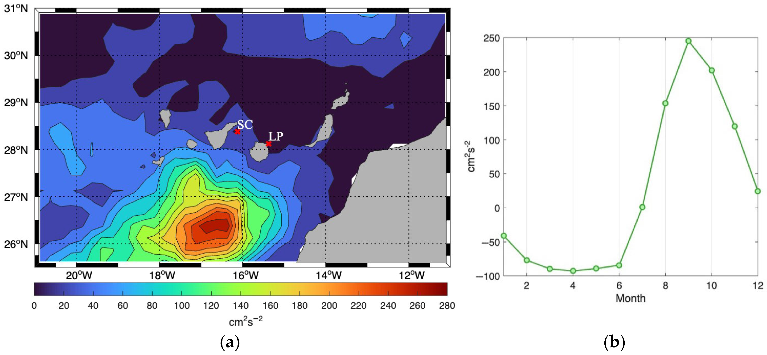
One such factor may be mesoscale activity, which is consistent with the intensification of eddies previously observed in the Canary Eddy Corridor over the past 30 years [42]. The seasonal variation in EKE, as shown in Figure 8a, reveals a broader range south of the Canary Islands, extending southwestward. This pattern is consistent with the previously observed intensification of eddies [43]. Studying the seasonality of EKE could help explain some of the variability in the spatial discrepancy between SST and sea level. Our results show that, similar to SST and sea level (Figure 6 and Figure 7), EKE maximum can be observed in September and October, with significant variations occurring along the southern edge of the study region between 25.5° and 28° N (Figure 8b).

3.4. Future Projections

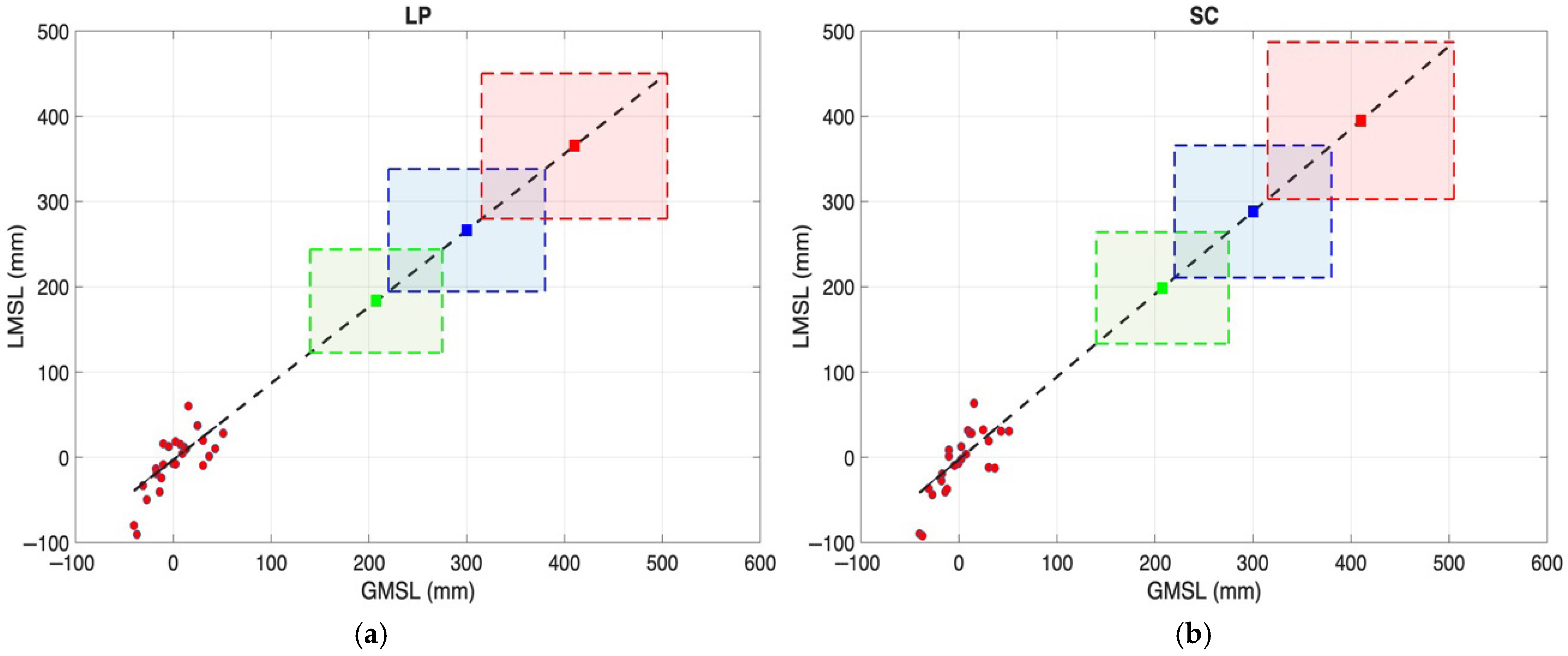
One of the objectives of this study is to estimate the expected mean sea level change in the Canary Islands by the middle of the 21st century, based on recent observational data analyzed in this paper. This projection relies on extrapolating the relationship between local sea level records, corrected for vertical land motion, and the most recent reconstructed GMSL time series into the future [12]. Assuming that the long-term local sea level rise will not necessarily be linear but rather proportional to global sea level rise, a linear relationship between local and global sea level series is expected [8]. The extrapolation can then be performed using a simple linear regression model, with the GMSL series as the input variable and the LMSL as the response variable (Figure 9).
We used three future scenarios proposed in the Sixth Assessment Report [1]—SSP1–1.9 (the most optimistic), SSP2–4.5, and SSP5–8.5 (the most pessimistic)—to estimate sea-level change up to 2050. These scenarios represent possible future climate trajectories based on demographic changes, economic development, urbanization patterns, greenhouse gas emissions, and the extent of climate intervention policies. The resulting projections (Figure 9 and Table 2) show a progressive rise in sea levels depending on the scenario. In the best-case scenario (SSP1–1.9), values close to 200 mm are reached, whereas in the worst-case scenario, values are near 400 mm. The estimates, which include uncertainty intervals, show that the LP station is slightly less sensitive than the SC station.
Nonetheless, the sea-level rise observed at both locations closely follows global projections.

4. Discussion

4.1. Long-Term Trend

Results from tide gauge and satellite altimetry data indicate a rising trend in sea level at both locations during the period 1993–2022. At the LP station, the trend is 4.04 ± 0.83 mm yr−1 based on tide gauge data, and 3.38 ± 0.41 mm yr−1 from altimetry. At the SC station, the corresponding values are 4.38 ± 0.93 mm yr−1 and 3.52 ± 0.45 mm yr−1, respectively. These rates are slightly higher than those obtained by Marrero-Betancor et al. [9] for the region from 1993 to 2019, as well as higher than those reported for the GMSL by Frederikse et al. [12], who estimated 3.35 ± 0.34 mm yr−1 for the period 1993–2018, and by Dangendorf et al. [14], who found 3.1 ± 0.3 mm yr−1 for 1993–2015.
The altimetry results reveal complex spatial variability in mean sea level rise at the scale of typical mesoscale processes. A closer inspection shows that relative minima south of the islands coincide with locations where cyclonic eddies are frequently observed, while relative maxima correspond to areas typically dominated by anticyclonic eddies [43,44,45,46,47,48], as approximately indicated in Figure 10. This finding is consistent with the observed positive trend in eddy kinetic energy (EKE) within the Canary Eddy Corridor, suggesting that the intensity of eddy activity has increased in this region over the study period, thereby influencing the spatial pattern of sea level trends. This finding aligns with the reported intensification of global ocean EKE over the past three decades, based on satellite altimetry observations [42].

4.2. Vertical Land Motion

Tide gauges typically exhibit stronger residual persistence (larger ϕ) than coastal altimetry, consistent with local processes that are muted in spatially averaged altimetry [36,37]. Subtracting the tide gauge series from the altimetry series serves as a proxy for vertical land motion. In our case, the differences are small and only weakly positive at SC (0.63 ± 0.55 mm/yr), though they are indistinguishable from zero at LP (0.46 ± 0.55 mm/yr). This indicates minor subsidence at most during the period from 1993 to 2022.
Several previous studies have also reported vertical land motion in the Canary Islands, although with varying results, as summarized in Table 3. Among them, Pfeffer & Allemand [22] and Barbero et al. [38] report significantly higher rates of subsidence, whereas GNSS data from the SONEL network and estimates from the PSMSL database yield values closer to ours, particularly for Tenerife. These discrepancies could be explained by methodological differences or limitations in data availability and temporal coverage.

4.3. Interannual Variability

Climate modes such as those represented by the NAO, the AMO, the EA pattern, and the AMOC significantly correlate with interannual sea level variability through coupled atmospheric and oceanic processes [49]. Our results indicate that, while some degree of relationship exists between sea level variations at the LP and SC tide gauges and these four climate indices, the strongest correlation is observed with the NAO, which shows correlation coefficients of 0.53 for LP and 0.61 for SC. The NAO’s direct modulation of regional atmospheric circulation patterns, including wind stress, storm track positioning, and pressure distribution over the North Atlantic, likely causes this strong correlation. These patterns can significantly affect coastal sea levels on interannual timescales.
The EA pattern also influences sea level variability, though to a lesser degree compared to the NAO, possibly due to its secondary role over the North Atlantic [50]. On the other hand, the AMO and the AMOC appear to be primarily linked to the lower-frequency component of sea level variability. This connection is consistent with the longer timescale at which both climate modes operate, involving deep ocean processes and large-scale meridional heat distribution. However, the AMO shows higher correlation coefficients either at LP (0.40) and SC (0.41) stations than the AMOC does. This frequency-dependent influence underscores the importance of considering different climatic drivers when interpreting regional sea level variability.

4.4. Seasonal Cycle

The seasonality of local sea level is primarily thermosteric (driven by temperature-induced expansion and contraction of seawater) with additional contributions from wind and atmospheric pressure [17,26]. Using gridded altimetry and sea-surface-temperature data for the Canary region, we find that monthly sea level and SST covary closely, consistent with Marrero-Betancor et al. [9]. However, the tide-gauge records exhibit larger seasonal amplitudes than the collocated 0.25° altimetry grid cells. This is expected because Level 4 gridded fields represent spatially averaged conditions and therefore smooth harbour-scale coastal signals. Moreover, tide gauges sample very local processes (harbour thermodynamics, wind setup, and inverse-barometer response) that are muted in the gridded altimetry. In the Canary eastern boundary setting, published analyses around Spain/NE Atlantic also report a strong steric control of the annual cycle offshore, with harbour signals potentially amplified by local dynamics [51].
However, the spatial analysis shows that this behaviour is not uniform across the archipelago. Differences in the magnitude and spatial distribution of the seasonal anomalies indicate that, in addition to temperature, other processes modulate sea level, plausibly linked to regional ocean dynamics [20]. In particular, mesoscale eddies have been proposed to influence sea level in the Canary region [52] and in other island systems such as Hawaii [53]. The seasonality of eddy kinetic energy (EKE) in our data is consistent with this interpretation. A rigorous partition of the seasonal signal into steric and dynamical components (including wind- and pressure-forced responses) would require targeted hydrographic observations and local atmospheric measurements, which is beyond the scope of this study.

4.5. Future Projections

The implementation of the IPCC’s SSP scenarios [1] for 2050 has allowed estimation of potential sea level rise at the two studied locations. Under the most pessimistic scenario (SSP5–8.5), projected sea level rise could exceed 390 mm in SC and 365 mm in LP. These figures slightly differ from the estimates provided by NASA’s Sea Level Projection Tool, summarized in Table 4.
The NASA projections for the more optimistic scenarios (equivalent to SSP1–1.9 and SSP2–4.5) are slightly higher than our estimates, although they present notably broader uncertainty margins. However, under the most pessimistic scenario (equivalent to SSP5–8.5), our results indicate a higher sea level rise compared to NASA’s estimates. Furthermore, it is noteworthy that NASA’s tool assigns identical values to both locations, despite the known spatial variability within the Canary region driven by local oceanographic processes and differential land subsidence. This suggests that NASA’s projections might be overly generalized for local-scale applications, whereas our study provides estimates with narrower error margins, consistent with the significant spatial variability observed in the Canary Islands.
Finally, it should be noted that if land subsidence continues, it will lead to an additional increase in relative sea level. Assuming a constant rate equal to that observed in this study, this would imply an extra rise of approximately 20 mm by 2050 at both the LP and SC stations.

5. Conclusions

This study provides a detailed analysis of mean sea level variability in the Canary Islands from 1993 to 2022 by combining tide gauge and satellite altimetry data. Comparisons with external projections confirm that the Canary Islands follow the global pattern of accelerated sea level rise [12,14] but they also exhibit discernible spatial heterogeneity. This heterogeneity appears closely linked to mesoscale ocean dynamics, particularly eddy activity within the Canary Eddy Corridor.
Vertical land motion contributes to the observed relative sea level trends, with subsidence detected at both locations. Although these rates are modest (~0.5–0.7 ± 0.55 mm yr−1), their effect accumulates over time and must be considered in local risk assessments.
Seasonal sea level variability appears to be primarily driven by steric effects, as evidenced by the close relationship between sea surface temperature (SST) and sea level. However, the spatial patterns of seasonal amplitude differ between SST and sea level, suggesting the involvement of additional oceanographic processes.
The study shows that interannual sea level variability is primarily correlated with the North Atlantic Oscillation (NAO). By contrast, variations in the Atlantic Multidecadal Oscillation (AMO) and the Atlantic Meridional Overturning Circulation (AMOC) seem to be linked only to lower-frequency components.
Future projections under different SSP scenarios show that sea level could rise as much as 395 mm in Santa Cruz and 365 mm in Las Palmas in 2050 under the most pessimistic emissions scenario (SSP5–8.5). An additional 20 mm could be added due to land subsidence if it remains constant. Since these projections do not fully match NASA estimates, they highlight the need for locally calibrated models that consider regional oceanographic processes and land motion.
In conclusion, the Canary Islands have a complex and dynamic sea level regime that cannot be fully understood through global averages. The influence of factors such as mesoscale processes, vertical land motion, and climatic modes could intensify local impacts, highlighting the necessity of ongoing monitoring and specific studies particularly under high-emission scenarios. Future work should further explore the role of mesoscale and seasonal processes and integrate high-resolution regional models with observational data. Enhanced long-term monitoring and localized projections will be essential for effective adaptation planning in this vulnerable region.

Author Contributions

Software, A.M.-M.; Writing—original draft, M.I.; Visualization, A.M.-M.; Supervision, A.M.-M. All authors have read and agreed to the published version of the manuscript.

Funding

This research received no external funding.

Data Availability Statement

The original contributions presented in this study are included in the article. Further inquiries can be directed to the corresponding author(s).

Conflicts of Interest

The authors declare no conflicts of interest.

Abbreviations

The following abbreviations are used in this manuscript:
AMOAtlantic Multidecadal Oscillation
AMOCAtlantic Meridional Overturning Circulation
CIConfidence Interval
CMEMSCopernicus Marine Environment Monitoring Service
DUACSData Unification and Altimeter Combination System
EAEast Atlantic Pattern
EKEEddy Kinetic Energy
ENSOEl Niño–Southern Oscillation
GLSGeneralized Least Squares
GMSLGlobal Mean Sea Level
GNSSGlobal Navigation Satellite System
IPCCIntergovernmental Panel on Climate Change
LMSLLocal Mean Sea Level
LPLas Palmas de Gran Canaria (Tide Gauge Station)
NAONorth Atlantic Oscillation
PDOPacific Decadal Oscillation
PSMSLPermanent Service for Mean Sea Level
SCSanta Cruz de Tenerife (Tide Gauge Station)
SSPShared Socioeconomic Pathways (IPCC Emission Scenarios)
SSTSea Surface Temperature

References

  1. IPCC. Climate Change 2023: Synthesis Report. In Contribution of Working Groups I, II and III to the Sixth Assessment Report of the Intergovernmental Panel on Climate Change; Core Writing Team, Lee, H., Romero, J., Eds.; IPCC: Geneva, Switzerland, 2023; p. 184. [Google Scholar] [CrossRef]
  2. Neumann, B.; Vafeidis, A.T.; Zimmermann, J.; Nicholls, R.J. Future Coastal Population Growth and Exposure to Sea-Level Rise and Coastal Flooding: A Global Assessment. PLoS ONE 2015, 10, e0118571. [Google Scholar] [CrossRef] [PubMed]
  3. Kopp, R.E.; Hay, C.C.; Little, C.M.; Mitrovica, J.X. Geographic Variability of Sea-Level Change. Curr. Clim. Change Rep. 2015, 1, 192–204. [Google Scholar] [CrossRef]
  4. Nicholls, R.J. Planning for the Impacts of Sea Level Rise. Oceanography 2011, 24, 144–157. [Google Scholar] [CrossRef]
  5. Stammer, D.; Cazenave, A.; Ponte, R.M.; Tamisiea, M.E. Causes for Contemporary Regional Sea Level Changes. Annu. Rev. Mar. Sci. 2013, 5, 21–46. [Google Scholar] [CrossRef]
  6. Woodworth, P.L.; Melet, A.; Marcos, M.; Ray, R.D.; Wöppelmann, G.; Sasaki, Y.N.; Cirano, M.; Hibbert, A.; Huthnance, J.M.; Monserrat, S.; et al. Forcing Factors Affecting Sea Level Changes at the Coast. Surv. Geophys. 2019, 40, 1351–1397. [Google Scholar] [CrossRef]
  7. Oppenheimer, M.; Glavovic, B.C.; Hinkel, J.; van de Wal, R.; Magnan, A.K.; Abd-Elgawad, A.; Cai, R.; Cifuentes-Jara, M.; DeConto, R.M.; Ghosh, T.; et al. Sea Level Rise and Implications for Low-Lying Islands, Coasts and Communities. In IPCC Special Report on the Ocean and Cryosphere in a Changing Climate; Pörtner, H.O., Roberts, D.C., Masson-Delmotte, V., Zhai, P., Tignor, M., Poloczanska, E., Mintenbeck, K., Alegría, A., Nicolai, M., Okem, A., et al., Eds.; Cambridge University Press: Cambridge, UK, 2019; pp. 321–445. [Google Scholar] [CrossRef]
  8. Fraile-Jurado, P.; Sánchez-Rodríguez, E.; Fernández-Díaz, M.; Pita, M.F.; López-Torres, J.M. Estimación del Comportamiento Futuro del Nivel del Mar en las Islas Canarias a partir del Análisis de Registros Recientes. Geographicalia 2014, 66, 79–98. [Google Scholar] [CrossRef]
  9. Marrero-Betancort, N.; Marcello, J.; Rodríguez-Esparragón, D.; Hernández-León, S. Sea Level Change in the Canary Current System during the Satellite Era. J. Mar. Sci. Eng. 2022, 10, 936. [Google Scholar] [CrossRef]
  10. Pugh, D.; Woodworth, P.L. Sea-Level Science: Understanding Tides, Surges, Tsunamis and Mean Sea-Level Changes; Cambridge University Press: Cambridge, UK, 2014. [Google Scholar]
  11. Biguino, B.; Haigh, I.D.; Antunes, C.; Lamas, L.; Tel, E.; Dias, J.M.; Brito, A.C. Seasonal Patterns, Inter-Annual Variability, and Long-Term Trends of Mean Sea Level along the Western Iberian Coast and the North Atlantic Islands. J. Geophys. Res. Oceans 2024, 129, e2023JC020742. [Google Scholar] [CrossRef]
  12. Frederikse, T.; Landerer, F.W.; Caron, L.; Adhikari, S.; Parkes, D.; Humphrey, V.W.; Dangendorf, S.; Hogarth, P.; Zanna, L.; Cheng, L.; et al. The Causes of Sea Level Rise since 1900. Nature 2020, 584, 393–397. [Google Scholar] [CrossRef]
  13. Church, J.A.; White, N.J.; Konikow, L.F.; Domingues, C.M.; Cogley, J.G.; Rignot, E.; Gregory, J.M.; van den Broeke, M.R.; Monaghan, A.J.; Velicogna, I. Revisiting the Earth’s Sea-Level and Energy Budgets from 1961 to 2008. Geophys. Res. Lett. 2011, 38, L18601. [Google Scholar] [CrossRef]
  14. Dangendorf, S.; Hay, C.; Calafat, F.M.; Marcos, M.; Piecuch, C.G.; Berk, K.; Jensen, J. Persistent Acceleration in Global Sea-Level Rise since the 1960s. Nat. Clim. Change 2019, 9, 705–710. [Google Scholar] [CrossRef]
  15. Ray, R.D.; Douglas, B.C. Experiments in Reconstructing Twentieth-Century Sea Levels. Prog. Oceanogr. 2011, 91, 496–515. [Google Scholar] [CrossRef]
  16. Hamlington, B.D.; Frederikse, T.; Nerem, R.S.; Fasullo, J.T.; Adhikari, S. Investigating the Acceleration of Regional Sea Level Rise during the Satellite Altimeter Era. Geophys. Res. Lett. 2020, 47, e2019GL086528. [Google Scholar] [CrossRef]
  17. Gregory, J.M.; White, N.J.; Church, J.A.; Bierkens, M.F.P.; Box, J.E.; van den Broeke, M.R.; Cogley, J.G.; Fettweis, X.; Hanna, E.; Huybrechts, P.; et al. Twentieth-Century Global-Mean Sea Level Rise: Is the Whole Greater than the Sum of the Parts? J. Clim. 2013, 26, 4476–4499. [Google Scholar] [CrossRef]
  18. Gregory, J.M.; Griffies, S.M.; Hughes, C.W.; Lowe, J.A.; Church, J.A.; Fukumori, I.; Gomez, N.; Kopp, R.E.; Landerer, F.; Le Cozannet, G.; et al. Concepts and Terminology for Sea Level: Mean, Variability and Change, Both Local and Global. Surv. Geophys. 2019, 40, 1251–1289. [Google Scholar] [CrossRef]
  19. Vermeer, M.; Rahmstorf, S. Global Sea Level Linked to Global Temperature. Proc. Natl. Acad. Sci. USA 2009, 106, 21527–21532. [Google Scholar] [CrossRef]
  20. Hamlington, B.D.; Gardner, A.S.; Ivins, E.; Lenaerts, J.T.M.; Reager, J.T.; Trossman, D.S.; Zaron, E.D.; Adhikari, S.; Arendt, A.; Aschwanden, A.; et al. Understanding of Contemporary Regional Sea-Level Change and the Implications for the Future. Rev. Geophys. 2020, 58, e2019RG000672. [Google Scholar] [CrossRef] [PubMed]
  21. Martínez-Asensio, A.; Wöppelmann, G.; Ballu, V.; Becker, M.; Testut, L.; Magnan, A.K.; Duvat, V.K.E. Relative Sea-Level Rise and the Influence of Vertical Land Motion at Tropical Pacific Islands. Glob. Planet. Change 2019, 176, 132–143. [Google Scholar] [CrossRef]
  22. Pfeffer, J.; Allemand, P. The Key Role of Vertical Land Motions in Coastal Sea Level Variations: A Global Synthesis of Multisatellite Altimetry, Tide Gauge Data and GPS Measurements. Earth Planet. Sci. Lett. 2016, 439, 39–47. [Google Scholar] [CrossRef]
  23. Nerem, R.S.; Chambers, D.P.; Choe, C.; Mitchum, G.T. Estimating Mean Sea Level Change from the TOPEX and Jason Altimeter Missions. Mar. Geod. 2010, 33 (Suppl. S1), 435–446. [Google Scholar] [CrossRef]
  24. Volkov, D.L.; van Aken, H.M. Annual and Interannual Variability of Sea Level in the Northern North Atlantic Ocean. J. Geophys. Res. Oceans 2003, 108, C63204. [Google Scholar] [CrossRef]
  25. Hamlington, B.D.; Leben, R.R.; Strassburg, M.W.; Nerem, R.S.; Kim, K.Y. Contribution of the Pacific Decadal Oscillation to Global Mean Sea Level Trends. Geophys. Res. Lett. 2013, 40, 5171–5175. [Google Scholar] [CrossRef]
  26. Forget, G.; Ponte, R.M. The Partition of Regional Sea Level Variability. Prog. Oceanogr. 2015, 137, 173–195. [Google Scholar] [CrossRef]
  27. van Westen, R.M.; Dijkstra, H.A. Ocean Eddies Strongly Affect Global Mean Sea-Level Projections. Sci. Adv. 2021, 7, 116. [Google Scholar] [CrossRef]
  28. Chen, J.L.; Wilson, C.R.; Tapley, B.D. Seasonal Global Water Mass Balance and Mean Sea Level Variations. Geophys. Res. Lett. 1998, 25, 3555–3558. [Google Scholar] [CrossRef]
  29. Vinogradov, S.V.; Ponte, R.M. Low-Frequency Variability in Coastal Sea Level from Tide Gauges and Altimetry. J. Geophys. Res. Oceans 2011, 116, C07006. [Google Scholar] [CrossRef]
  30. Hughes, C.W.; Williams, S.D.P. The Color of Sea Level: Importance of Spatial Variations in Spectral Shape for Assessing the Significance of Trends. J. Geophys. Res. Oceans 2010, 115, C10048. [Google Scholar] [CrossRef]
  31. Holgate, S.J.; Matthews, A.; Woodworth, P.L.; Rickards, L.J.; Tamisiea, M.E.; Bradshaw, E.; Foden, P.R.; Gordon, K.M.; Jevrejeva, S.; Pugh, J. New Data Systems and Products at the Permanent Service for Mean Sea Level. J. Coast. Res. 2013, 29, 493–504. [Google Scholar] [CrossRef]
  32. Permanent Service for Mean Sea Level (PSMSL). Tide Gauge Data. 2025. Available online: http://www.psmsl.org/data/obtaining/ (accessed on 28 April 2025).
  33. Pérez, B.; Payo, A.; López, D.; Woodworth, P.L.; Álvarez Fanjul, E. Overlapping Sea Level Time Series Measured Using Different Technologies: An Example from the REDMAR Spanish Network. Nat. Hazards Earth Syst. Sci. 2014, 14, 589–610. [Google Scholar] [CrossRef]
  34. Pérez Gómez, B.; Aarup, T.; Bradshaw, E.; Illigner, J.; Matthews, A.; Mitchell, B.; Rickards, L.; Stone, P.; Widlansky, M.; Williams, J. Quality Control of in situ Sea Level Observations: A Review and Progress towards Automated Quality Control. In IOC Manuals and Guides; Intergovernmental Oceanographic Commission of UNESCO: Paris, France, 2020; Volume 1, p. 71. [Google Scholar]
  35. Copernicus Marine Environment Monitoring Service (CMEMS) Marine Data Store (MDS). Global Ocean Gridded L4 Sea Surface Heights and Derived Variables Reprocessed Copernicus Climate Service. Available online: https://data.marine.copernicus.eu/product/SEALEVEL_GLO_PHY_L4_MY_008_047/description (accessed on 4 April 2025).
  36. Ballarotta, M.; Ubelmann, C.; Pujol, M.I.; Taburet, G.; Fournier, F.; Legeais, J.F.; Faugère, Y.; Dibarboure, G. On the Resolutions of Ocean Altimetry Maps. Ocean Sci. 2019, 15, 1091–1109. [Google Scholar] [CrossRef]
  37. Williams, J.; Hughes, C. The Coherence of Small Island Sea Level with the Wider Ocean. Ocean Sci. 2013, 9, 111–119. [Google Scholar] [CrossRef]
  38. Barbero, I.; Torrecillas, C.; Páez, R.; Prates, G.; Berrocoso, M. Recent Macaronesian Kinematics from GNSS Ground Displacement Analysis. Stud. Geophys. Geod. 2021, 65, 15–35. [Google Scholar] [CrossRef]
  39. NASA. NASA Sea Level Change Portal: Sea Level Projection Tool. Available online: https://sealevel.nasa.gov/ipcc-ar6-sea-level-projection-tool (accessed on 28 April 2025).
  40. Bos, M.S.; Williams, S.D.P.; Araújo, I.B.; Bastos, L. The Effect of Temporal Correlated Noise on the Sea Level Rate and Acceleration Uncertainty. Geophys. J. Int. 2014, 196, 1423–1430. [Google Scholar] [CrossRef]
  41. Bos, M.S.; Montillet, J.P.; Williams, S.D.P.; Fernandes, R.M.S. Introduction to Geodetic Time Series Analysis. In Geodetic Time Series Analysis in Earth Sciences; Montillet, J.P., Bos, M., Eds.; Springer Geophysics; Springer: Cham, Switzerland, 2020; pp. 29–52. [Google Scholar] [CrossRef]
  42. Barceló-Llull, B.; Rosselló, P.; Combes, V.; Sánchez-Román, A.; Pujol, M.I.; Pascual, A. Robust Intensification of Global Ocean Eddy Kinetic Energy from Three Decades of Satellite Altimetry Observations. arXiv 2024, arXiv:2406.08014. [Google Scholar] [CrossRef]
  43. Sangrà, P.; Pascual, A.; Rodríguez-Santana, Á.; Machín, F.; Mason, E.; McWilliams, J.C.; Pelegrí, J.L.; Dong, C.; Rubio, A.; Arístegui, J.; et al. The Canary Eddy Corridor: A Major Pathway for Long-Lived Eddies in the Subtropical North Atlantic. Deep-Sea Res. Part I Oceanogr. Res. Pap. 2009, 56, 2100–2114. [Google Scholar] [CrossRef]
  44. Arístegui, J.; Sangrà, P.; Hernández-León, S.; Cantón, M.; Hernández-Guerra, A.; Kerling, J.L. Island-Induced Eddies in the Canary Islands. Deep Sea Res. Part I Oceanogr. Res. Pap. 1994, 41, 1509–1525. [Google Scholar] [CrossRef]
  45. Sangrà, P.; Pelegrí, J.L.; Hernández-Guerra, A.; Arregui, I.; Martín, J.M.; Marrero-Díaz, A.; Martínez, A.; Ratsimandresy, A.W.; Rodríguez-Santana, A. Life History of an Anticyclonic Eddy. J. Geophys. Res. Oceans 2005, 110, C03021. [Google Scholar] [CrossRef]
  46. Sangrà, P.; Auladell, M.; Marrero-Díaz, A.; Pelegrí, J.L.; Fraile-Nuez, E.; Rodríguez-Santana, A.; Martín, J.M.; Mason, E.; Hernández-Guerra, A. On the Nature of Oceanic Eddies Shed by the Island of Gran Canaria. Deep Sea Res. Part I Oceanogr. Res. Pap. 2007, 54, 687–709. [Google Scholar] [CrossRef]
  47. Barceló-Llull, B.; Sangrà, P.; Pallàs-Sanz, E.; Barton, E.D.; Estrada-Allis, S.N.; Martínez-Marrero, A.; Aguiar-González, B.; Grisolía, D.; Gordo, C.; Rodríguez-Santana, A.; et al. Anatomy of a Subtropical Intrathermocline Eddy. Deep-Sea Res. Part I Oceanogr. Res. Pap. 2017, 124, 126–139. [Google Scholar] [CrossRef]
  48. Cerdán-García, E.; Álvarez-Salgado, X.A.; Arístegui, J.; Martínez-Marrero, A.; Benavides, M. Eddy-Driven Diazotroph Distribution in the Subtropical North Atlantic: Horizontal Variability Prevails over Particle Sinking Speed. Commun. Biol. 2024, 7, 929. [Google Scholar] [CrossRef]
  49. Han, W.; Meehl, G.A.; Stammer, D.; Hu, A.; Hamlington, B.; Kenigson, J.; Palanisamy, H.; Thompson, P. Spatial Patterns of Sea Level Variability Associated with Natural Internal Climate Modes. Surv. Geophys. 2017, 38, 217–250. [Google Scholar] [CrossRef]
  50. Martínez-Asensio, A.; Marcos, M.; Tsimplis, M.N.; Gomis, D.; Josey, S.; Jordà, G. Impact of the Atmospheric Climate Modes on Mediterranean Sea Level Variability. Glob. Planet. Change 2014, 118, 1–15. [Google Scholar] [CrossRef]
  51. García-Lafuente, J.; del Río, J.; Álvarez Fanjul, E.; Gomis, D.; Delgado, J. Some Aspects of the Seasonal Sea Level Variations around Spain. J. Geophys. Res. Oceans 2004, 109, C09008. [Google Scholar] [CrossRef]
  52. Navarro-Pérez, E.; Barton, E.D. Seasonal and Interannual Variability of the Canary Current. Sci. Mar. 2001, 65 (Suppl. S1), 205–213. [Google Scholar] [CrossRef]
  53. Firing, Y.L.; Merrifield, M.A. Extreme Sea Level Events at Hawaii: Influence of Mesoscale Eddies. Geophys. Res. Lett. 2004, 31, L24306. [Google Scholar] [CrossRef]
Figure 1. Study area and bathymetry. The markers indicate the locations of the tide gauges at Las Palmas de Gran Canaria (LP) and Santa Cruz de Tenerife (SC).
Jmse 13 02193 g001
Figure 2. Global mean sea level (GMSL) time series including quadratic trend based on the reconstruction by Frederikse et al. [12] for the period 1900–2018. The altimetry era is indicated.
Jmse 13 02193 g002
Figure 3. Tide gauge and nearby grid-cell altimetry data for (a) Las Palmas (LP) and (b) Santa Cruz (SC), showing monthly means, annual means, and linear trends for the period 1993–2022. Time series are referenced to mean sea level for the period 1995–2014, same reference level used by IPCC in its last Assessment Report (AR6). Black dots indicate gaps in the tide gauge records.
Jmse 13 02193 g003
Figure 4. Sea level trend in the Canary Islands region for the period 1993–2022. The locations of nearby tide gauges grid-cells are highlighted as well.
Jmse 13 02193 g004
Figure 5. Interannual normalized sea level anomalies (-MSL*, in black) in (a) LP and (b) SC for the period 1993–2022 compared with four detrended climate indices: from top to bottom NAO*, AMO*, EA* pattern and AMOC*.
Jmse 13 02193 g005
Figure 6. (a,b) seasonal sea level anomalies derived from tide gauges (blue lines) and satellite altimetry at the grid cells nearest to the tide gauges (red lines); (c) spatially averaged satellite altimetry over the entire study area.
Jmse 13 02193 g006
Figure 7. (a) Range of the seasonal oscillation in sea level across the entire study area; (b) seasonal SST spatial changes; (c,d) range of (c) sea level and (d) SST seasonal cycle across the entire study area for the period 1993–2022.
Jmse 13 02193 g007
Figure 8. Eddy Kinetic Energy (EKE) seasonal shifts in the Canary Islands region for the period 1993–2022 expressed in cm2s−2. (a) Spatial distribution of seasonal changes; (b) range of these changes across the study area. The locations of nearby tide gauges grid-cells are highlighted as well.
Jmse 13 02193 g008
Figure 9. Regression between local mean sea level rise at (a) Las Palmas de Gran Canaria and (b) Santa Cruz de Tenerife, and GMSL. The dashed line represents the linear relationship extrapolated to 2050. Colored squares show projected mean sea level ranges under SSP1–1.9 (green), SSP2–4.5 (blue), and SSP5–8.5 (red).
Jmse 13 02193 g009
Figure 10. Sea level trend in the Canary Islands region for the period 1993–2022, with the approximate frequent locations of cyclonic (C) and anticyclonic (A) eddies indicated, based on observations reported in the literature [42,44,45,46,47].
Jmse 13 02193 g010
Table 1. Local sea level rise trends at LP and SC (1993–2022), and vertical land motion inferred from the difference between tide-gauge and altimetry records. Values are in mm yr−1 ± 95% confidence interval; in parentheses, we report the AR(1) coefficient ϕ estimated from the GLS fit.
LPSC
Tide gauge trend4.04 ± 0.83 (0.83)4.38 ± 0.93 (0.85)
Altimetry trend3.38 ± 0.41 (0.62)3.52 ± 0.45 (0.59)
Difference0.51 ± 0.55 (0.66)0.69 ± 0.55 (0.41)
Table 2. Projected mean sea level rise by 2050 for LP and SC tide gauges expressed in mm. The results for three SSP scenarios, along with their associated uncertainties, are shown.
LPSC
SSP1–1.9182.78 ± 60.47202.40 ± 66.67
SSP2–4.5265.63 ± 71.67293.76 ± 79.01
SSP5–8.5364.18 ± 85.11402.40 ± 93.83
Table 3. Summary of vertical land motion results obtained from previous studies and databases, compared with the present study. The results are expressed in mm yr−1, including their uncertainty intervals and the corresponding time periods.
LPSCPERIOD
PFEFFER & ALLEMAND [22]−1.92 ± 0.48−2.48 ± 0.331992–2013
BARBERO ET AL. [34]−1.68 ± 0.81−2.40 ± 0.392000–2015 (LP) 2008–2015 (SC)
GNSS (SONEL)Not robust−1.55 ± 0.202007–2014
PSMSLNot robust−0.59 ± 0.32007–2023
PRESENT STUDY−0.51 ± 0.55−0.69 ± 0.551993–2022
Table 4. Comparison of mean sea level rise projections estimated in the present study with those provided by NASA for the same locations (LP and SC) and Shared Socioeconomic Pathways (SSP 1.9, 4.5, and 8.5). The results are expressed in mm, including their uncertainty intervals. Note that NASA obtains same results for both locations.
SCENARIONASA PROJECTION FOR 2050 (LP AND SC)LPSC
SSP1–1.9260 (170–360)183.22 ± 60.62198.60 ± 65.45
SSP2–4.5280 (190–380)266.29 ± 71.85288.29 ± 77.57
SSP5–8.5310 (220–400)365.08 ± 85.32394.94 ± 92.11
Disclaimer/Publisher’s Note: The statements, opinions and data contained in all publications are solely those of the individual author(s) and contributor(s) and not of MDPI and/or the editor(s). MDPI and/or the editor(s) disclaim responsibility for any injury to people or property resulting from any ideas, methods, instructions or products referred to in the content.