Water-State-Aware Spatiotemporal Graph Transformer Network for Water-Level Prediction

Abstract

Accurate water-level prediction is a critical component for ensuring safe maritime navigation, optimizing port operations, and mitigating coastal flooding risks. However, the complex, non-linear spatiotemporal dynamics of water systems pose significant challenges for current forecasting models. The proposed framework introduces three key innovations. First, a dual-weight graph construction mechanism integrates geographical proximity with Dynamic Time Warping (DTW)-derived temporal similarity to better represent hydrodynamic connectivity in coastal and estuarine environments. Second, a state-aware weighted loss function is designed to enhance predictive accuracy during critical hydrological events, such as storm surges and extreme tides, by prioritizing the reduction in errors in these high-risk periods. Third, the WS-STGTN architecture combines graph attention with temporal self-attention to capture long-range dependencies in both space and time. Extensive experiments are conducted using water-level data from five stations in the tidal-influenced lower Yangtze River, a vital artery for shipping and a region susceptible to coastal hydrological extremes. The results demonstrate that the model consistently surpasses a range of baseline methods. Notably, the WS-STGTN achieves an average reduction in Mean Squared Error (MSE) of 27.6% compared to the standard Transformer model, along with the highest coefficient of determination ($R^2\approx 0.96$) across all datasets, indicating its stronger explanatory power for observed water-level variability. This work provides a powerful tool that can be directly applied to improve coastal risk management, marine navigation safety, and the operational planning of port and coastal engineering projects.

1. Introduction

Accurate water-level prediction in coastal waterways and navigation channels is crucial for effective, safe navigation, port operations, and coastal risk management under complex environments [1]. The manager or ship officer generally judges the water depth situation of a channel based on prediction values from the water level station to ensure navigation safety and decide on ship navigation planning [2]. However, the water level changing trend in the water level station is impacted by nearby water level situations. Surrounding environmental changes, such as changing amounts of water from upstream, periodic changes in tides, or regulation of reservoirs from dams, directly influence the trend of water level of a specific station near coastal areas [3]. The majority of conventional algorithms have focused only on training models based on historical water-level sequential data [4]. They have not paid attention to upstream and downstream influences on water-level change trends, especially in water level stations near the sea. Inaccurate prediction of water levels would decrease the efficiency of vessel navigation and increase risks during vessel navigation, especially for ports that manage vessels when anchoring based on tide changes and water levels in channels. Underutilized channel depths due to inaccurate prediction of the depth of channels can cost millions in delayed shipments and suboptimal cargo loading [5]. At the same time, coastal water-level predictions are core reference data for controlling risks during vessel navigation in coastal areas, which assists in identifying safely navigable areas in complex environments. Therefore, these limitations directly or indirectly impact the navigation safety of vessels, port operations, and coastal risk management in marine and estuarine systems.

Furthermore, the intensification of hydrological extremes under climate change, represented as increasingly severe floods and droughts, poses a critical threat to the safety and efficiency of waterway transportation [6]. Precise and real-time water level predictions provide operational convenience in terms of ship navigation and management of ports or channels. This advancement plays a vital role in the adaption of traffic management systems. It empowers rerouting of vessels in response to rapidly fluctuating conditions [7]. Taking, as an example, a historic event on the Rhine River in 2021, approximately 200 vessels were grounded in the Rhine River, crippling this critical European supply corridor and triggering estimated economic losses exceeding 5 billion euros within a single month [8,9]. These catastrophic events highlight the critical importance of developing advanced adaptive frameworks for water-level prediction during extreme hydrological periods. Thus, accurate and timely forecasts are essential to ensure maritime safety, maintain logistical continuity, and mitigate severe financial and ecological consequences.

In aspect of algorithms regarding water level prediction, the traditional statistical approaches for water level forecasting, exemplified by the Autoregressive Integrated Moving Average (ARIMA) model, rely heavily on physical and statistical principles but often struggle to capture the dynamic, nonlinear complexities inherent in hydrological systems. For instance, Yu et al. [10] applied ARIMA to provide satisfactory short-term daily water level forecasts for flood control, shipping, and water supply management. Its accuracy decreased significantly during periods of sharp water level fluctuations and as the forecasting period extended, which highlights the limitation in capturing complex non-linear dynamics and maintaining performance over longer lead times. While conventional machine learning methods offer greater flexibility, they inadequately represent the complex spatiotemporal dependencies across water level stations. The studies [11,12] utilized Support Vector Machines (SVM) and its variant to forecast the multi-step water level in the Yangtze River. They achieved the good short-term accuracy yet revealed the difficulties in capturing long-term temporal patterns and spatial interactions between distant gauges without explicit feature engineering. On the other hand, deep learning techniques have gained prominence due to their ability of automatically extracting relevant spatiotemporal features. Zhang et al. [13] developed a hybrid model with convolutional neural network and long short-term memory network to predict downstream water level prediction of reservoir. It significantly improved the computation efficiency and had superior forecasting ability to the benchmark methods. However, these advanced deep learning methods still face challenges regarding generalization under non-stationary conditions and often necessitate significant volumes of high-quality training data and support of high-performance processor.

At the same time, accurate water level prediction is critically dependent on capturing both complex temporal dynamics and inherent spatial inter-dependencies, as water levels at any station are influenced by upstream conditions, lateral inflows, and downstream backwater effects within the watershed system. However, the current popular pattern of building model—ranging from discussed statistical methods to conventional deep learning—often inadequately represent these essential spatial linkages and hydrodynamic constraints. They primarily focused on temporal patterns at discrete points or relied on the simplified spatial interpolations, which leads to systemic errors in capturing basin-wide hydrodynamic interactions. This limitation is acutely evident in coastal area and channel nearby sea where downstream stage-flow relationships are highly dynamic. Consequently, the modeling framework with an explicit topology to represent the connection and influential relationship among water level stations is necessary. To address the limitations of algorithms above discussed and meet the critical need for accurate water level predictions, we propose the Water State-aware Spatiotemporal Graph Transformer Network (WS-STGTN) to achieve task of water level prediction. It maps the topology to represent the relationship among water level in aspect of spatial and temporal features. The water level stations in the topology are set as the interconnected nodes. The water level monitoring points are formalized as the vertex Their edge weights are designed by similarity between geographical distance and time series features. This framework in the proposed model is designed to enhance water level prediction capabilities across navigation channels and overcome the fragmented representation inherent in current discrete or interpolation-based approaches. The contributions of this study are summarized in the following key points:

• A framework using dual-weight edge construction mechanism is designed, which integrates geographical distance and temporal correlation, yielding a more holistic representation of the interplay among water level stations.
• A state-aware weighted loss function is introduced, which not only dynamically adjusts the importance of prediction errors based on different water level states, but also ensures the accuracy during critical periods.
• A graph transformer network based on theory of transformer is designed, which employs the advanced attention mechanisms to focus on the relevant information and model complex dependencies.
• A precise water level prediction model—WS-STGTN—is proposed, which assists on the safe navigation, port operations, and coastal risk management under complex environment.

In the following sections, Section 2 will outline our methodology in detail, including the definition of water level states, the construction of the graph structure. Section 3 will provide the implementation and evaluation of the WS-STGTN. Section 4 will introduce dataset description, experimental settings, evaluation metrics, and details of experiments. The following Section 5 will show the experimental results and their discussion. Section 6 will conclude our findings and the implications of our work for waterway management and maritime safety.

2. Literature Review

Accurate water level prediction is crucial for effective water resource management, flood risk mitigation, and the safety and efficiency of navigation systems. Over the years, a variety of methodologies have been developed, evolving from traditional statistical models to machine learning, deep learning, and more recently, graph-based and Transformer models, with increasing attention on capturing complex spatiotemporal dynamics across rivers, lakes, and estuarine systems.

Early water level forecasting relied primarily on statistical approaches such as the Autoregressive Integrated Moving Average (ARIMA) model. ARIMA captures linear temporal dependencies using historical observations, providing straightforward interpretability and computational efficiency. Adnan et al. [14] applied ARIMA to streamflow forecasting and observed improved performance compared to alternative models in terms of mean absolute percentage error (MAPE) and root mean square error (RMSE). Similarly, Yu et al. [10] demonstrated ARIMA’s utility for Yangtze River water level prediction. Nevertheless, ARIMA assumes linear relationships and stationary time series, which limits its ability to model nonlinear dynamics and abrupt fluctuations, especially during extreme events [15].

To address the limitations of linear models, machine learning (ML) methods have been widely adopted, including Support Vector Machines (SVM), Random Forests (RF), and Gradient Boosting (GB). These models can handle nonlinear dependencies and large datasets. Castillo-Botón et al. [16] demonstrated that Support Vector Regression (SVR) achieved high precision in reservoir inflow forecasting, while Tran et al. [17] found RF maintained robust performance for river water level prediction even with missing data. Gradient boosting methods, particularly XGBoost, have been enhanced through hybridization with evolutionary algorithms, outperforming RF and CART in multi-step water level prediction [18]. Despite these advantages, ML models require careful feature selection and engineering; improper inputs or hyperparameter tuning may lead to overfitting and limited generalization in complex hydrological systems.

Deep learning (DL) techniques, including Long Short-Term Memory (LSTM) networks and Convolutional Neural Networks (CNN), have been increasingly employed to model temporal and spatial dependencies. LSTM effectively captures long-term temporal correlations but can be sensitive to transitional hydrological dynamics, reducing performance in medium-term predictions [19]. Hybrid methods integrating signal decomposition techniques such as Variational Mode Decomposition (VMD) enable separation of dominant trends, seasonal cycles, and high-frequency noise, which are subsequently modeled using sequence-aware predictors like LSTM [20,21]. CNNs extract spatial features from sensor grids or watershed maps and can be fused with attention-enhanced LSTM to jointly capture temporal and spatial patterns, improving forecasting accuracy [22]. These approaches have also been applied to lake-level prediction, e.g., Xu et al. [23] used Transformer models to simulate Poyang Lake water levels with high accuracy, demonstrating the potential of DL in both river and lake systems. However, challenges remain, including high computational cost, dependence on large labeled datasets, and potential oversimplification of complex watershed interactions [24,25].

A key limitation of prior approaches is the decoupling of temporal and spatial dependencies. Recent work has addressed this using graph neural networks (GNN) and Transformer architectures. ST-GNN and GCN-LSTM models have effectively captured spatiotemporal interactions in groundwater and river networks, outperforming standalone LSTM and traditional numerical models [26,27,28]. Transformer-based models, including BiLSTM-Transformer and ladder-Transformer frameworks, have shown superior accuracy in multi-step water level prediction for lakes and rivers, often exceeding conventional RNN-based architectures [29,30,31]. Hybrid DL architectures integrating CNN, LSTM, GRU, and Transformer components further enhance robustness and forecasting precision across various temporal scales and monitoring stations [32,33,34]. Additionally, these models have been extended to flow prediction, capturing temporal variations in streamflow and estuarine dynamics, which is crucial for flood early warning and reservoir operation [14,18].

Despite these advances, critical challenges remain. Most current methodologies focus on individual monitoring stations, neglecting the influence of surrounding hydrological and environmental factors. Temporal and spatial features are often treated separately, limiting models’ ability to capture dynamic interactions among water levels across stations, particularly in heterogeneous and complex coastal environments. Conventional loss functions uniformly weight prediction errors, ignoring the operational significance of different water level states (e.g., flood alerts vs. normal conditions). Standard graph networks frequently lack adaptive mechanisms to discern contextually relevant spatiotemporal dependencies from noisy multivariate data, reducing reliability during extreme events.

To address these deficiencies, this study proposes the WS-STGTN framework for monitoring-point water level prediction. The framework dynamically fuses temporal correlations with spatial proximity to capture synergistic effects on water propagation across hydrological networks. It incorporates state-aware optimization by applying differential weighting in the loss function, reflecting the operational importance of various water level states. Transformer-based attention mechanisms enable adaptive graph learning, allowing the model to identify contextually relevant spatiotemporal dependencies from noisy multivariate data. By integrating these strategies, WS-STGTN enhances both predictive accuracy and robustness, particularly during extreme hydrological events. A detailed description of the proposed methodology is provided in the following section.

3. Methodology

This study aims to deliver accurate monitoring point of water level in the coastal area while minimizing reliance on external data, WS-STGTN is introduced. First, a data-driven spatio-temporal graph is constructed. Hydrological stations and selected points with water level data are nodes (geographic coordinates as static attributes, historical water-level series as dynamic attributes) and edges are weighted by inferred hydrological connectivity. Second, a Graph Transformer is trained on this evolving graph;  its multi-head self-attention simultaneously models spatial dependencies across stations and temporal dynamics within each station, directly producing future water-level sequences. Last, a state-aware weighted Mean Squared Error (WMSE) loss function is designed, which provides the different weights for forecasting errors for samples belonging to different hydrological states (e.g., flood, normal, and drought).

3.1. Data Transformation Approach

To prepare raw multi-station water level series for model training, a sliding-window transformation is applied. Let $\mathbf{Z}\in {\mathbb{R}}^{T\times N}$ denote water level data from N monitoring stations over T time steps. Given an input window size D and a prediction horizon P, training samples are generated as

$$X_{\mathrm{train}}\in {\mathbb{R}}^{L\times D\times N},{\mathcal{Y}}_{\mathrm{train}}\in {\mathbb{R}}^{L\times P\times N},$$

(1)

where L is the number of training instances. Each $X_{\mathrm{train}}$ contains D sequential observations, and the corresponding ${\mathcal{Y}}_{\mathrm{train}}$ contains the following P target values. This structure facilitates temporal pattern learning across multiple stations.

3.2. Water Level State Definition

To capture hydrological variability, historical water levels are categorized into three regimes—flood, typical, and drought—using the k-means clustering algorithm. Given observed levels $X=\{x_1,x_2,\dots ,x_n\}$, the objective is

$$\underset{{\left\{C_k\right\}}_{k=1}^3}{min}\sum _{k=1}^3\sum _{x_i\in C_k}{\parallel x_i-{\mu }_k\parallel }^2,$$

(2)

where ${\mu }_k$ is the centroid of cluster $C_k$. After convergence, clusters are ordered by centroid values and assigned state labels $s_i\in \{\mathrm{flood},\mathrm{typical},\mathrm{drought}\}$. These labels later serve to adaptively weight prediction errors in the model loss function (Section 3.4), improving accuracy during extreme conditions.

3.3. Dynamic Spatio-Temporal Graph Model

The accurate representation of hydrological interdependencies requires explicit modeling of both spatial connectivity and temporal dynamics. This subsection details our dual-approach methodology for capturing these complex relationships through integrated geographical and temporal similarity measures.

A dynamic graph structure is represented as $\mathcal{G}=(\mathcal{V},\mathcal{E},\mathcal{W})$, where the vertex set $\mathcal{V}=\{v_1,v_2,\dots ,v_N\}$, the edge set is $\mathcal{E}$, and $\mathcal{W}$ represents the edge weights. In our study, the water level monitoring points are formalized as the vertex in graph structure and the historical features in water level series is set as corresponding nodes features. Their edge weights are designed by similarity between geographical distance and time series features, which reflects the significance of influence between monitoring points. The adjacency matrix $\mathbf{A}\in {[0,1]}^{N\times N}$ encodes pairwise relationships where ${\mathbf{A}}_{ij}=w_{ij}$ quantifies the influence of station j on point i.

First, the spatial connectivity matrix captures fundamental relationships of monitoring points driven by geographical proximity. We employ a multi-step computational process to transform raw coordinates into normalized connection weights that reflect hydrodynamic interdependence. The Haversine formula computes great-circle distances between stations i and j with coordinates (${\varphi }_i,{\lambda }_i$) and (${\varphi }_j,{\lambda }_i$). The distance computation can be showed in Equation (3).

$$\begin{array}{cc}\hfill \Delta \varphi & =|{\varphi }_j-{\varphi }_i|{\displaystyle \frac{\pi }{180}},\hfill \\ \hfill \Delta \lambda & =|{\lambda }_j-{\lambda }_i|{\displaystyle \frac{\pi }{180}},\hfill \\ \hfill a& ={sin}^2\left({\displaystyle \frac{\Delta \varphi }{2}}\right)+cos\left({\varphi }_i{\displaystyle \frac{\pi }{180}}\right)cos\left({\varphi }_j{\displaystyle \frac{\pi }{180}}\right){sin}^2\left({\displaystyle \frac{\Delta \lambda }{2}}\right),\hfill \\ \hfill D(i,j)& =2\times 6371\times arctan\left(\sqrt{a},\sqrt{1-a}\right).\hfill \end{array}$$

(3)

where Earth’s radius R = 6371 km and angular differences are converted to radians. This formula calculates the great-circle distance between two geographic coordinates on the Earth’s surface, and the use of the $arctan(\sqrt{a},\sqrt{1-a})$ function ensures numerical stability for small angular separations.

Then, this study applies a normalized exponential decay function to convert distances into connectivity weights. Its mathematical representation is showed in the following:

$$w_{(i,j)}={\displaystyle \frac{exp(-\beta ·\tilde{d}(i,j))-exp(-\beta )}{exp\left(0\right)-exp(-\beta )}}$$

(4)

Here, $\tilde{d}(i,j)$ is linearly scaled into [0, 1], and $\beta$ controls the decay rate of spatial influence; a higher $\beta$ leads to faster attenuation of long-range connections.

The waterway topology is generated through directional constraints. The weights can be updated by following equation:

$$w_{(i,j)}=\left\{\begin{array}{cc}{w}_{(i,j)}·{\rho }_{ij}\hfill & \mathrm{if}j\mathrm{is}\mathrm{upstream}\mathrm{of}i\hfill \\ 0.5·w_{(i,j)}·{\rho }_{ij}\hfill & \mathrm{if}j\mathrm{is}\mathrm{downstream}\mathrm{of}i\hfill \\ 0\hfill & \mathrm{otherwise}\hfill \end{array}\right.$$

(5)

where ${\rho }_{ij}=exp\left(-{\displaystyle \frac{\Delta h}{L}}\right)$ represents the elevation difference ($\Delta h$) and river length L between points, which enforces much stronger weights for upstream connections. The spatial weights can be generated by Equation (6).

$$A={\displaystyle \frac{1}{\left|\mathcal{E}\right|}}\sum _{(i,j)\in \mathcal{E}}{w}_{(i,j)}$$

(6)

Here, A represents the normalized spatial adjacency strength of the graph, obtained by averaging all valid edge weights in $\mathcal{E}$; this ensures that the overall connectivity is scale-invariant and comparable across different Network.

On the other hand, considering the delay effect of water flow propagation, conventional Pearson correlation fails to account for phase misalignment in hydrograph comparisons. Thus, we employ Dynamic Time Warping (DTW) to quantify the morphological congruence between water level series $T{S}_i$ and $T{S}_j$, accommodating the hydraulic time lags inherent in watershed response dynamics. The smaller value of the DTW distance $d_{DTW}(i,j)$ indicates the more similar the morphologies of the two sequences are. This study converts it into time-dependent weights through the Gaussian kernel function as Equation (7).

$$w_{\mathrm{time}}(i,j)=exp\left(-{\displaystyle \frac{d_{\mathrm{DTW}}{(i,j)}^2}{2{\sigma }^2}}\right)$$

(7)

where $d_{\mathrm{DTW}}(i,j)$ represents the DTW distance between the water level time series of stations i and j, and $\sigma$ is an adjustable hyperparameter used to control the sensitivity of the DTW distance to weight attenuation. A higher $\sigma$ value reduces the decay rate of the similarity weight function, implying that significant hydrological correlations may persist between stations despite substantial DTW distances.

Finally, the edge weights integrate spatial proximity and hydrograph congruence through a convex combination of geographical and temporal similarity metrics. Its mathematical representation is showed in Equation (8).

$$w_{\mathrm{combined}}(i,j)=\alpha ·w_{\mathrm{distance}}(i,j)+(1-\alpha )·w_{\mathrm{time}}(i,j)$$

(8)

where $\alpha$ is a hyperparameter between 0 and 1, used to balance the relative importance of geographical distance weights and temporal correlation weights. The larger value of $\alpha$ represents the more important the geographical distance is in determining the correlation between sites. All the combined weights form the adjacency matrix $\mathbf{A}$ of the graph, where ${\mathbf{A}}_{ij}=w_{\mathrm{combined}}(i,j)$.

3.4. WS-STGTN Model Architecture

Water State Spatio-Temporal Graph Transformer Network (WS-STGTN) employs a hierarchical encoder-decoder structure to model complex hydrological dependencies. The architecture integrates spatial topology and temporal dynamics through specialized attention mechanisms, enabling precise water level forecasting across interconnected water level monitoring points.

The encoder layer employs a dual-pathway attention mechanism to capture spatio-temporal dependencies inherent in hydrological systems. The spatial pathway utilizes a graph attention network that incorporates the adjacency matrix $A\in R^{N\times N}$ that is generated by Section 3.3. The attention mechanism works by comparing the features of the target node i with the features of each of its neighbors j to determine the importance of each neighbor. The core operation for calculating the unnormalized attention score $e_{ij}$ by Equation (9).

$$e_{ij}=\mathrm{LeakyReLU}\left({\mathbf{a}}^T[{\mathbf{W}}_g{\mathbf{x}}_i\parallel {\mathbf{W}}_g{\mathbf{x}}_j]\right)$$

(9)

where ${\mathbf{W}}_g\in {\mathbb{R}}^{d\times d}$ is the shared projection matrix for feature transformation; $\mathbf{a}\in {\mathbb{R}}^{2d}$ represents the attention mechanism weight vector. Then, the attention score is normalized by Equation (10) and is represented as ${\alpha }_{ij}$, which defines how much influence station j has on station i.

$${\alpha }_{ij}={\displaystyle \frac{exp\left(e_{ij}\right)}{{\sum }_{k\in \mathcal{N}\left(i\right)}exp\left(e_{ik}\right)}}$$

(10)

For each node i, the spatial aggregation is computed below equation:

$${\mathbf{h}}_i^{\mathrm{spat}}=\sigma \left(\sum _{j\in \mathcal{N}\left(i\right)}{\alpha }_{ij}{\mathbf{W}}_v{\mathbf{x}}_j\right)+{\mathbf{x}}_i$$

(11)

where ${\mathbf{W}}_v\in {\mathbb{R}}^{d\times d}$ is the projection matrix; and $A_{ij}$ is the adjacency weight.

At the same time, the long-range temporal dependencies within each monitoring point’s water level time series, we employ a causal self-attention mechanism. This component allows the model to dynamically weigh the importance of past observations when generating representations for future predictions. The mechanism begins by transforming the input temporal input that are generated by data transformation approach into three distinct semantic spaces through learned linear projections. Its mathematical representation is showed in the following:

$${\mathbf{Q}}_t={\mathbf{X}}_t{\mathbf{W}}_Q,{\mathbf{K}}_t={\mathbf{X}}_t{\mathbf{W}}_K,{\mathbf{V}}_t={\mathbf{X}}_t{\mathbf{W}}_V$$

(12)

where X are the input features generated by data transformation approach, ${\mathbf{W}}_Q$, ${\mathbf{W}}_K$, and ${\mathbf{W}}_V$ are learnable weights in the proposed model. Then, multi-head temporal self-attention is computed as:

$${\mathrm{Att}}_t=\mathrm{softmax}\left({\displaystyle \frac{Q_t{K}_t^{\top }}{\sqrt{d_k}}}\right)V_t$$

(13)

These attention maps capture temporal dependencies at different representation subspaces, enabling the model to focus on diverse patterns of temporal correlation across multiple heads. The outputs from all heads are then concatenated and linearly transformed as follows:

$$H^{(\ell -1)}=\mathrm{Concat}\left({\mathrm{Att}}_1,\dots ,{\mathrm{Att}}_H\right)W^O$$

(14)

where $W^O$ are learnable parameters, and Concat(·) function represents the concatenation among output of the different heads of attention.

The WS-STGTN model progressively extracts and integrates spatial dependencies and temporal dynamics within the water level data by above processing through multiple stacked spatio-temporal encoder layers. Each encoder layer first aggregates information from neighboring stations via a graph attention mechanism (GAT), generating spatially context-aware node representations. Next, a temporal self-attention mechanism captures long-range dependencies within the sequence, enhancing the model’s ability to represent temporal patterns at each station. The node representations output by the final encoder layer are then fed into a fully-connected output network to predict water levels for the next P time steps.

To achieve the water level state awareness, a Weighted Mean Squared Error (WMSE) loss function is designed. This function assigns different weights to the prediction error of each sample based on the water level state (determined by the K-means clustering results in Section 3.2) to which the true water level $y_i$ belongs. The loss function is formulated as:

$$Loss={\displaystyle \frac{1}{N}}\sum _{i=1}^N\left[w{(y_i-{\widehat{y}}_i)}^2\right]$$

(15)

where w denotes the weight assigned according to the water level state (i.e., dry, normal, or flood) of $y_i$. Higher weights are allocated to samples from flood and dry periods (e.g., $w_{\mathrm{flood}}>w_{\mathrm{normal}}$ and $w_{\mathrm{dry}}>w_{\mathrm{normal}}$), thereby directing the model to focus more on prediction accuracy during these critical hydrological phases. By minimizing this WMSE loss, the model is optimized to not only reduce overall prediction errors but also prioritize performance in states that are hydrologically sensitive or operationally significant, ultimately enhancing the practical reliability and state-specific perception capability of the forecasting system. The entire model is trained in an end-to-end manner by minimizing a loss function. The pseudocode is shown in Algorithm 1, which shows the detail of training process in model WS-STGTN. To visualize this multi-stage process, the overall architecture of the proposed WS-STGTN is illustrated in Figure 1.

Algorithm 1: WS-STGTN Model Process

Require: Historical water level time series for all stations: ${\left\{X_i\right\}}_{i=1}^N$ where $X_i=[x_{i,t-D+1},\dots ,x_{i,t}]$ Ensure: Predicted water levels for future P time steps: $\widehat{Y}=[{\widehat{y}}_{i,t+1},\dots ,{\widehat{y}}_{i,t+P}]$ for each station i 1: Initialize model parameters: graph attention weights $\mathbf{W}$, $\mathbf{a}$, and temporal self-attention parameters 2: for$l=1$ to L do 3:    Graph Attention Module (GAT) in layer l: 4:    for each node i do 5:      for each neighbor $j\in {\mathcal{N}}_i$ do 6:         Compute attention coefficient $e_{ij}$ by Equation (9); 7:      end for 8:      Normalize coefficients by Equation (10); 9:      Aggregate neighbor features (${\mathbf{h}}_i^{\mathrm{spat}}$) by Equation (11); 10:    end for 11:    Update node representations: ${\mathbf{H}}^{\left(\mathrm{GAT}\right)}=[{\mathbf{h}}_1^{\mathrm{spat}},\dots ,{\mathbf{h}}_N^{\mathrm{spat}}]$; 12:    Temporal Self-Attention Module in layer l: 13:    for each node i do 14:      Project inputs to queries, keys, valuesby Equation (12); 15:      Compute attention by Equation (13); 16:      Apply multi-head mechanism by Equation (14); 17:    end for 18:    Update node representations: ${\mathbf{H}}^{\left(l\right)}=[{\mathbf{H}}_1^{\left(\mathrm{l}\right)},\dots ,{\mathbf{H}}_N^{\left(\mathrm{l}\right)}]$ 19: end for 20: Output layer: Pass final representations ${\mathbf{H}}^{\left(L\right)}$ through a fully connected layer: $\widehat{Y}=\mathrm{FC}\left({\mathbf{H}}^{\left(L\right)}\right)$; 21: Calculate loss value based on WMSE loss function by Equation (15); 22: Update learnable parameters in the model until meet the stop condition; 23: return $\widehat{Y}$

4. Experiments

This section mainly compares the performance of the proposed WS-STGTN with that of representative baselines and ablated variants for multi-step water-level forecasting on a downstream reach of the Yangtze River. The details on the data description, experimental Settings, and performance measurement are provided in the following subsections.

4.1. Dataset Description

To evaluate multi-step water-level forecasting performance and examine the contribution of state-aware learning and dynamic spatio-temporal graph modeling, we employ five real-world water-level time series from the lower Yangtze River, China: Xinsheng–Hehai (XS–HH), Qingjiang Tidal Station (QJ), Sanjiangkou (SJK), Yizheng–Hehai (YZ–HH), and Dadao Estuary (DDE). Precise geographic coordinates are available for all stations (see Figure 2). After basic quality control, we retain the common observation window shared by all sites, from 21 June 2020 03:00:00 to 7 June 2023 03:00:00, sampled hourly. The fused hourly series therefore contains 26,088 timestamps per station; applying a 120-step encoder window together with a 24-step forecasting horizon yields $L=25,945$ sliding samples for model development.

Table 1. Station-wise descriptive statistics over the synchronized hourly window.

Station	Mean (m)	Min (m)	Max (m)	Std Dev (m)
XS–HH Station	3.14	0.17	7.51	1.68
QJ Station	3.06	0.15	7.87	1.67
SJK Station	2.85	0.50	7.20	1.55
YZ–HH Station	2.75	0.02	7.25	1.53
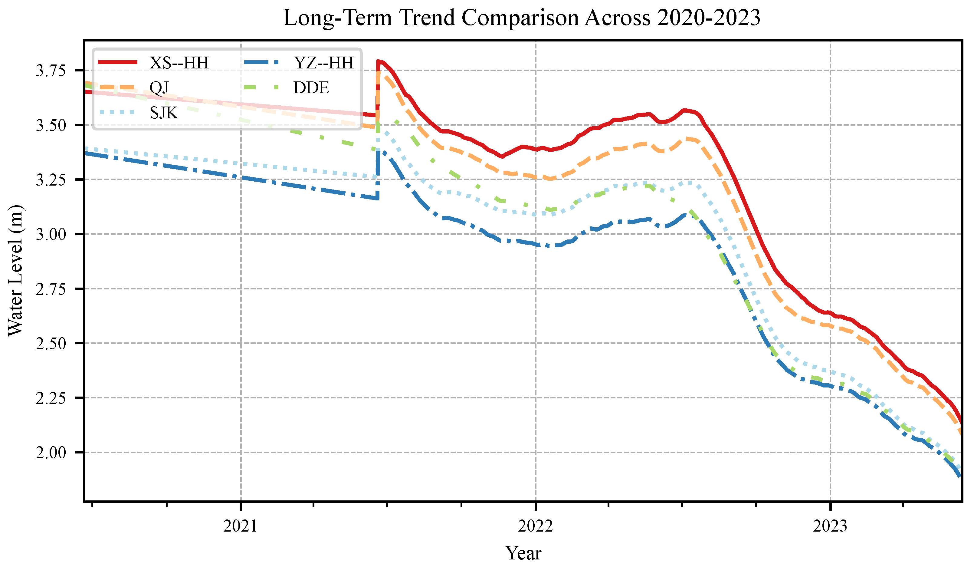
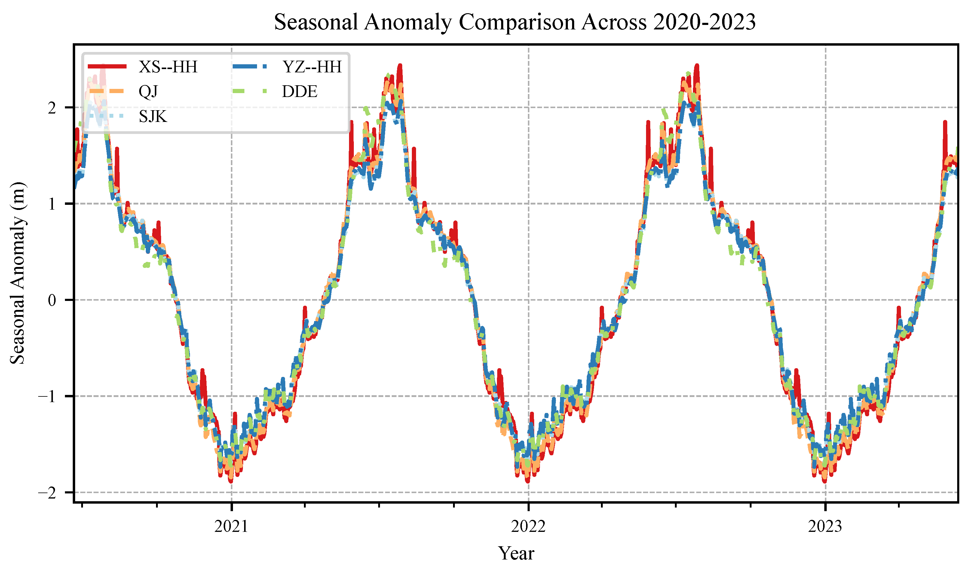
DDE Station	2.84	0.03	7.37	1.60

shows that mean water levels stay between 2.75 m and 3.14 m, while the minima (0.02–0.50 m), maxima (7.20–7.87 m), and standard deviations (1.53–1.68 m) are tightly clustered, demonstrating comparable fluctuation magnitudes along the reach. The trend signatures in Figure 3 rise and fall synchronously, and the seasonal anomaly profiles in Figure 4 share the same annual cycle with summer surges and winter recessions, confirming that the selected window captures representative upstream–downstream dynamics and tide-river interactions.

Following the data transformation described in Section 3, across all stations, this yields $L=25,945$ sliding windows. For convenience in downstream experiments, we also provide a flattened representation as a $25,945\times 144$ matrix). Equivalently, the transformed representation is $X\in {\mathbb{R}}^{L\times D\times N}$ and $Y\in {\mathbb{R}}^{L\times P\times N}$, with $N=5$ and $L=25,945$.

4.2. Experimental Settings

To validate the effectiveness and robustness of WS-STGTN across diverse forecasting horizons, model capacities, and graph configurations, we design experiments that first establish multi-step-ahead prediction baselines by benchmarking against widely used alternatives from statistics, machine learning, and deep learning, including ARIMA, SVR, LSTM, GCN, STGCN, and Transformer. In addition, to quantify the contribution of key architectural components in a spatiotemporal setting, we conduct ablation studies on a graph-based variant by constructing four controlled models: removing DTW-based temporal similarity in graph construction (NoDTW), replacing the proposed weighted MSE with standard MSE (NoWMSE), substituting graph attention with graph convolution (NoGAT), and replacing temporal self-attention with LSTM (NoTimeAttn).

We explore multiple combinations of the prediction horizon P and time window D tailored to each dataset. Unless otherwise specified, we set $P=24$ and $D=120$, and performance across four prediction horizons: 1–7, 8–16, 17–24, and 1–24. All time series are transformed following Liu [35]. All experiments use the common observation window described in Section 4 with a chronological split of 70% for training and 30% for testing. To ensure fair comparisons, we perform grid-search hyperparameter tuning to minimize MSE, focusing on a single principal hyperparameter per model: ARIMA selects the order $(p,d,q)$ by AIC within $p\in \{0,\dots ,4\}$, $d\in \{0,1,2\}$, $q\in \{0,\dots ,4\}$; SVR tunes the penalty $C\in \{1,10,100\}$; LSTM tunes the number of hidden units $\{64,128\}$; GCN tunes the number of layers $\{2,3\}$ using the adjacency A from Section 3.3; STGCN tunes the temporal kernel size $\{3,5\}$; the Transformer tunes the number of attention heads $\{4,8\}$. For WS-STGTN, we tune the graph balance parameter $\alpha \in \{0.4,0.6,0.8\}$ in Equation (8).

All experiments are conducted with Python 3.6.10 and PyTorch 1.7.1 (GPU build, CUDA 10.1) on an Intel(R) Core(TM) i7-8750H @ 2.20 GHz with 16 GB memory (Intel Corporation, Santa Clara, CA, USA). Reproducibility is ensured by fixing random seeds and preserving the chronological split to avoid information leakage. We report a set of complementary metrics for each prediction horizon, including MSE (Mean Squared Error), MAPE (Mean Absolute Percentage Error). These metrics collectively provide a comprehensive assessment of forecasting performance, capturing both absolute and relative errors. Detailed definitions of each metric are provided in the following subsection.

4.3. Performance Measurement

To comprehensively evaluate the forecasting performance of all models, we use two metrics. The Mean Absolute Percentage Error (MAPE) expresses prediction errors as a percentage of actual values:

$$\mathit{MAPE}={\displaystyle \frac{100\%}{N}}\sum _{i=1}^N{\displaystyle \frac{\left|{\widehat{y}}_i-y_i\right|}{\left|y_i\right|}}.$$

(16)

The Mean Squared Error (MSE) computes the average squared deviation, placing greater weight on larger errors:

$$\mathrm{MSE}={\displaystyle \frac{1}{N}}\sum _{i=1}^N{\left({\widehat{y}}_i-y_i\right)}^2.$$

(17)

Here, N denotes the number of observations, ${\widehat{y}}_i$ the predicted value, and $y_i$ the actual value.

Additionally, the coefficient of determination ($R^2$) is utilized to assess the proportion of variance explained by the model:

$$R^2=1-{\displaystyle \frac{{\sum }_{i=1}^N{({\widehat{y}}_i-y_i)}^2}{{\sum }_{i=1}^N{(y_i-\overline{y})}^2}},$$

(18)

where $\overline{y}$ denotes the mean of the observed values. $R^2$ provides a normalized measure of model fit, enabling comparison across datasets with differing ranges and scales.

5. Results and Discussion

5.1. Forecasting Performance Comparison

Table 2. Performance comparison of the proposed WS-STGTN and baseline models (SVR, LSTM, STGCN, Transformer) on five real-world Yangtze River water level datasets.

Dataset	Model	MSE				MAPE (%)				${\mathit{R}}^2$
		1–8	9–16	17–24	1–24	1–8	9–16	17–24	1–24	1–8	9–16	17–24	1–24
	SVR	$1.35\times {10}^{-1}$	$1.20\times {10}^{-1}$	$1.37\times {10}^{-1}$	$1.30\times {10}^{-1}$	21.90	18.17	20.44	20.17	0.79	0.81	0.79	0.80
	LSTM	$5.38\times {10}^{-2}$	$7.39\times {10}^{-2}$	$7.63\times {10}^{-2}$	$6.80\times {10}^{-2}$	8.96	12.04	12.38	11.13	0.92	0.88	0.88	0.89
XS–HH	STGCN	$7.09\times {10}^{-2}$	$9.76\times {10}^{-2}$	$1.08\times {10}^{-1}$	$9.21\times {10}^{-2}$	10.15	12.99	15.10	12.75	0.89	0.85	0.83	0.86
	Transformer	$5.58\times {10}^{-2}$	$6.99\times {10}^{-2}$	$7.52\times {10}^{-2}$	$6.70\times {10}^{-2}$	9.40	12.32	11.49	11.07	0.91	0.89	0.88	0.90
	WS-STGTN	$\mathbf{4}.\mathbf{42}\times {\mathbf{10}}^{-\mathbf{2}}$	$\mathbf{5}.\mathbf{73}\times {\mathbf{10}}^{-\mathbf{2}}$	$\mathbf{6}.\mathbf{51}\times {\mathbf{10}}^{-\mathbf{2}}$	$\mathbf{5}.\mathbf{55}\times {\mathbf{10}}^{-\mathbf{2}}$	6.99	8.76	9.50	8.42	0.93	0.91	0.90	0.91
	SVR	$1.20\times {10}^{-1}$	$9.73\times {10}^{-2}$	$9.07\times {10}^{-2}$	$1.02\times {10}^{-1}$	24.95	21.20	19.57	21.91	0.80	0.84	0.85	0.83
	LSTM	$1.98\times {10}^{-2}$	$3.30\times {10}^{-2}$	$3.84\times {10}^{-2}$	$3.04\times {10}^{-2}$	8.70	11.87	13.22	11.26	0.97	0.95	0.94	0.95
QJ	STGCN	$3.16\times {10}^{-2}$	$5.09\times {10}^{-2}$	$5.80\times {10}^{-2}$	$4.68\times {10}^{-2}$	8.79	11.91	13.51	11.40	0.95	0.92	0.90	0.92
	Transformer	$2.20\times {10}^{-2}$	$2.46\times {10}^{-2}$	$3.00\times {10}^{-2}$	$2.56\times {10}^{-2}$	7.61	9.29	10.20	9.03	0.96	0.96	0.95	0.96
	WS-STGTN	$\mathbf{1}.\mathbf{24}\times {\mathbf{10}}^{-\mathbf{2}}$	$\mathbf{2}.\mathbf{04}\times {\mathbf{10}}^{-\mathbf{2}}$	$\mathbf{2}.\mathbf{44}\times {\mathbf{10}}^{-\mathbf{2}}$	$\mathbf{1}.\mathbf{91}\times {\mathbf{10}}^{-\mathbf{2}}$	5.80	7.87	8.68	7.45	0.98	0.97	0.96	0.97
	SVR	$9.18\times {10}^{-2}$	$7.12\times {10}^{-2}$	$6.94\times {10}^{-2}$	$7.75\times {10}^{-2}$	23.11	18.45	17.63	19.73	0.84	0.87	0.87	0.86
	LSTM	$2.48\times {10}^{-2}$	$4.42\times {10}^{-2}$	$5.25\times {10}^{-2}$	$4.05\times {10}^{-2}$	10.26	15.51	17.54	14.44	0.96	0.92	0.91	0.93
SJK	STGCN	$3.19\times {10}^{-2}$	$5.09\times {10}^{-2}$	$5.98\times {10}^{-2}$	$4.76\times {10}^{-2}$	10.34	13.57	15.56	13.15	0.94	0.91	0.89	0.91
	Transformer	$2.84\times {10}^{-2}$	$2.90\times {10}^{-2}$	$3.58\times {10}^{-2}$	$3.11\times {10}^{-2}$	9.40	10.37	11.36	10.37	0.95	0.95	0.94	0.94
	WS-STGTN	$\mathbf{1}.\mathbf{43}\times {\mathbf{10}}^{-\mathbf{2}}$	$\mathbf{2}.\mathbf{18}\times {\mathbf{10}}^{-\mathbf{2}}$	$\mathbf{2}.\mathbf{56}\times {\mathbf{10}}^{-\mathbf{2}}$	$\mathbf{2}.\mathbf{06}\times {\mathbf{10}}^{-\mathbf{2}}$	7.04	8.91	9.54	8.49	0.97	0.96	0.95	0.96
	SVR	$1.15\times {10}^{-1}$	$1.02\times {10}^{-1}$	$1.02\times {10}^{-1}$	$1.06\times {10}^{-1}$	30.12	27.88	27.48	28.49	0.80	0.82	0.82	0.81
	LSTM	$2.82\times {10}^{-2}$	$4.26\times {10}^{-2}$	$7.05\times {10}^{-2}$	$4.71\times {10}^{-2}$	12.25	16.76	23.91	17.64	0.95	0.92	0.87	0.92
YZ–HH	STGCN	$3.39\times {10}^{-2}$	$5.70\times {10}^{-2}$	$6.77\times {10}^{-2}$	$5.29\times {10}^{-2}$	11.62	15.87	18.41	15.30	0.94	0.90	0.88	0.91
	Transformer	$3.11\times {10}^{-2}$	$3.97\times {10}^{-2}$	$4.25\times {10}^{-2}$	$3.78\times {10}^{-2}$	13.00	15.83	15.13	14.65	0.95	0.93	0.92	0.93
	WS-STGTN	$\mathbf{1}.\mathbf{56}\times {\mathbf{10}}^{-\mathbf{2}}$	$\mathbf{2}.\mathbf{37}\times {\mathbf{10}}^{-\mathbf{2}}$	$\mathbf{2}.\mathbf{87}\times {\mathbf{10}}^{-\mathbf{2}}$	$\mathbf{2}.\mathbf{27}\times {\mathbf{10}}^{-\mathbf{2}}$	7.58	9.97	11.14	9.57	0.97	0.96	0.95	0.96
	SVR	$1.16\times {10}^{-1}$	$9.02\times {10}^{-2}$	$8.76\times {10}^{-2}$	$9.79\times {10}^{-2}$	29.53	24.39	23.38	25.77	0.79	0.84	0.84	0.82
	LSTM	$2.63\times {10}^{-2}$	$4.07\times {10}^{-2}$	$4.17\times {10}^{-2}$	$3.63\times {10}^{-2}$	11.10	14.78	15.60	13.83	0.95	0.93	0.92	0.93
DDE	STGCN	$3.35\times {10}^{-2}$	$5.34\times {10}^{-2}$	$6.33\times {10}^{-2}$	$5.01\times {10}^{-2}$	10.99	14.46	16.76	14.07	0.94	0.90	0.88	0.91
	Transformer	$2.43\times {10}^{-2}$	$3.45\times {10}^{-2}$	$3.86\times {10}^{-2}$	$3.25\times {10}^{-2}$	8.83	11.03	12.09	10.65	0.96	0.94	0.93	0.94
	WS-STGTN	$\mathbf{1}.\mathbf{83}\times {\mathbf{10}}^{-\mathbf{2}}$	$\mathbf{2}.\mathbf{72}\times {\mathbf{10}}^{-\mathbf{2}}$	$\mathbf{3}.\mathbf{10}\times {\mathbf{10}}^{-\mathbf{2}}$	$\mathbf{2}.\mathbf{55}\times {\mathbf{10}}^{-\mathbf{2}}$	7.75	9.93	10.74	9.47	0.97	0.95	0.94	0.95

reports the forecasting performance of the proposed WS-STGTN and representative baselines on the five real-world Yangtze River water-level datasets (XS–HH, QJ, SJK, YZ–HH, DDE). Performance is evaluated in terms of MSE, MAPE and $R^2$ across different forecast horizons (1–8, 9–16, 17–24, and 1–24 steps).

On the full $1–24$ horizon, WS-STGTN reduces MSE by an average of $27.6\%$ and MAPE by $21.1\%$ relative to the Transformer, with the largest gains on YZ–HH and SJK. Relative to LSTM, average improvements are $37\%$ for MSE and $35\%$ for MAPE, underscoring the benefits of explicitly modeling spatiotemporal dependencies and lag-aware inter-station relations beyond sequence-only architectures. Across horizons, the gains are consistent, with the short and medium ranges $\left(1–8\mathrm{and}9–16\right)$ seeing the strongest boosts, while the long range $\left(17–24\right)$ still benefits notably. Compared with the graph-based STGCN, WS-STGTN delivers clear additional gains on $1–24$ of about $52\%$ lower MSE and $35\%$ lower MAPE on average, highlighting the value of lag-aware graph construction and dual attention through graph attention and temporal self-attention over static convolutional aggregation. Against classical SVR, the margins are very large. Furthermore, the coefficient of determination ($R^2$) consistently validates the superiority of WS-STGTN in capturing hydrological dynamics. Across all five stations, WS-STGTN attains the highest $R^2$ values, averaging around 0.95–0.97 on the full $1–24$ horizon, surpassing Transformer (0.93–0.94), LSTM (0.92–0.93), and STGCN (0.90–0.91). This improvement indicates that WS-STGTN not only minimizes prediction errors but also explains a substantially greater proportion of the observed variance in water-level fluctuations. The gains are especially evident at complex stations such as YZ–HH and DDE, where nonlinear flow interactions and lagged dependencies are prominent. These results confirm that the proposed model generalizes well under different hydrological regimes, achieving both lower error magnitudes and higher explanatory power.

5.2. Statistical Analysis

In this subsection, we evaluate the proposed WS-STGTN model by comparing its performance with that of other state-of-the-art forecasting methods widely recognized for their effectiveness in multistep prediction. The contenders include SVR, TCN, LSTM, GRU, and Transformer. To ensure a fair and comprehensive evaluation, all models are trained and tested under identical experimental settings using the benchmark hydrological datasets across multiple forecasting horizons (1–24 steps). The detailed results are summarized in Table 2, from which it can be observed that WS-STGTN consistently yields the lowest prediction error across all time horizons.

To further verify whether these improvements stem from systematic differences rather than random variations, we convert the Mean Absolute Percentage Error (MAPE) metric into an equivalent accuracy measure as follows:

$$\mathrm{Accuracy}=100\%-\mathrm{MAPE}.$$

(19)

Subsequently, we rank the five models based on their Accuracy for each dataset and forecasting horizon, assigning rank 1 to the worst-performing model and rank 5 to the most accurate one. To ensure a comprehensive statistical comparison, we apply the Quade test independently to both the Mean Squared Error (MSE) and Accuracy (i.e., $100\%-\mathrm{MAPE}$) metrics, thereby evaluating the consistency of model rankings across different performance criteria. This analysis determines whether the observed differences among models are statistically significant rather than attributable to random variability.

For the MSE metric, the Quade statistic yields $F(4,16)=18.000$ with a corresponding p-value of $9.01\times {10}^{-6}$, thereby rejecting the null hypothesis of equal median performance among models. As shown in Figure 5a, WS-STGTN attains a weighted mean rank close to 1.0, confirming its superiority over the competing methods, whereas SVR consistently ranks lowest. When Accuracy—a monotonic transformation of MAPE—is analyzed, the Quade test reports $F(4,16)=14.092$ with $p=4.13\times {10}^{-5}$, yielding an identical ranking pattern across all models (Figure 5b). Because Accuracy and MAPE produce equivalent rank sequences, the MAPE-based panel is omitted for brevity.

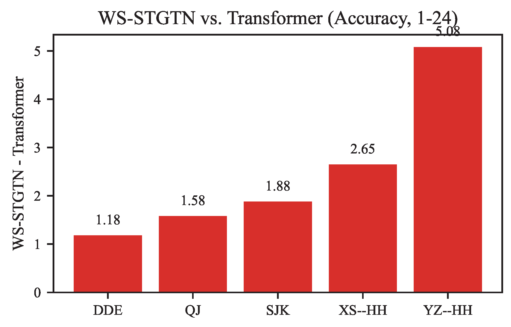
To further quantify the pairwise advantage of WS-STGTN over the strongest neural baseline, Transformer, we conduct a nonparametric sign test based on per-dataset Accuracy gains. The performance differences are summarized in

Table 3. Pairwise sign test comparing WS-STGTN and Transformer based on Accuracy across all forecasting horizons (1–24 steps). Positive differences indicate datasets where WS-STGTN outperforms Transformer.

Dataset	Transformer	WS-STGTN	Sign	Difference	Rank
DDE	89.350	90.530	+	1.180	1
QJ	90.970	92.550	+	1.580	2
SJK	89.630	91.510	+	1.880	3
XS–HH	88.930	91.580	+	2.650	4
YZ–HH	85.350	90.430	+	5.080	5

and visualized in Figure 6. In every case, WS-STGTN surpasses Transformer, yielding accuracy improvements ranging from 1.18% to 5.08%. The sign test produces five positive outcomes and no negatives, resulting in $p=0.0625$ due to the limited number of paired samples. Despite this marginal p-value, the uniformly positive differences strongly corroborate that the architectural innovations of WS-STGTN consistently enhance forecasting accuracy across all hydrological stations.

5.3. Visualization of Forecasts

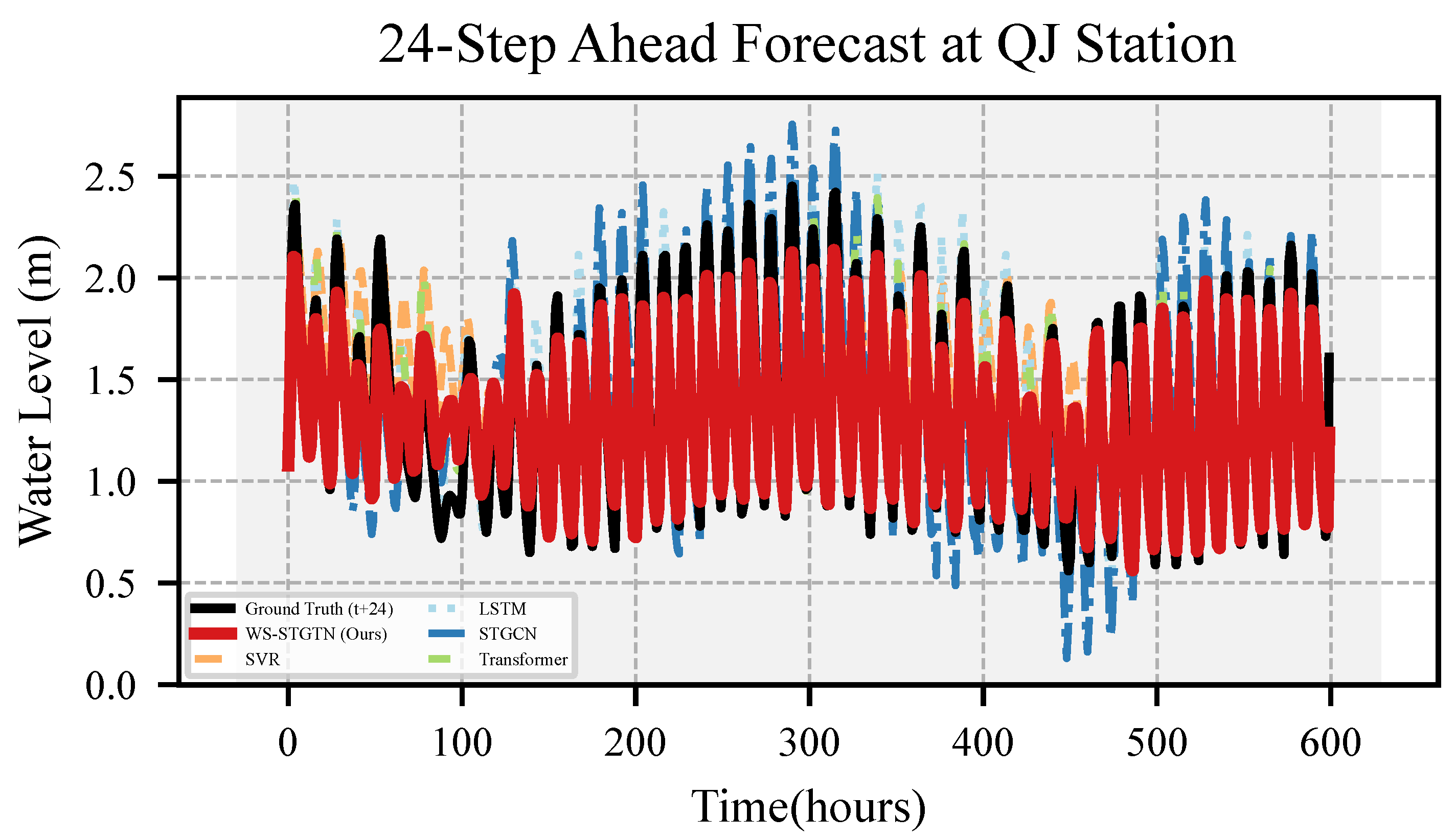
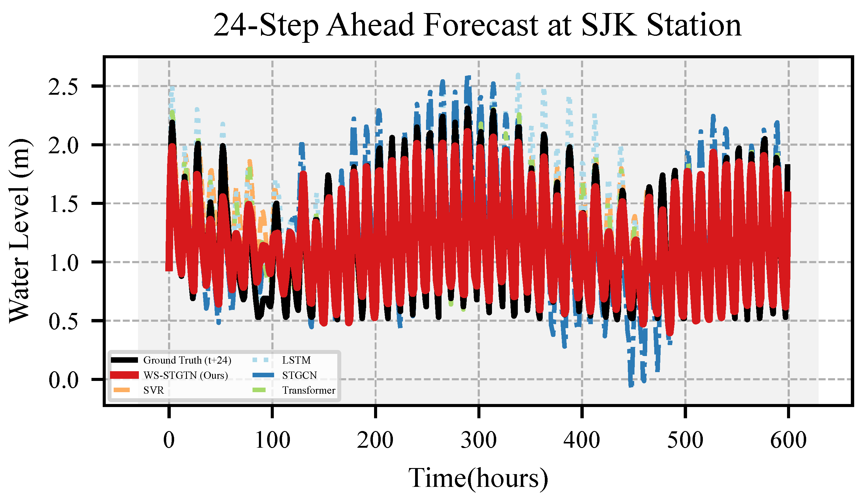
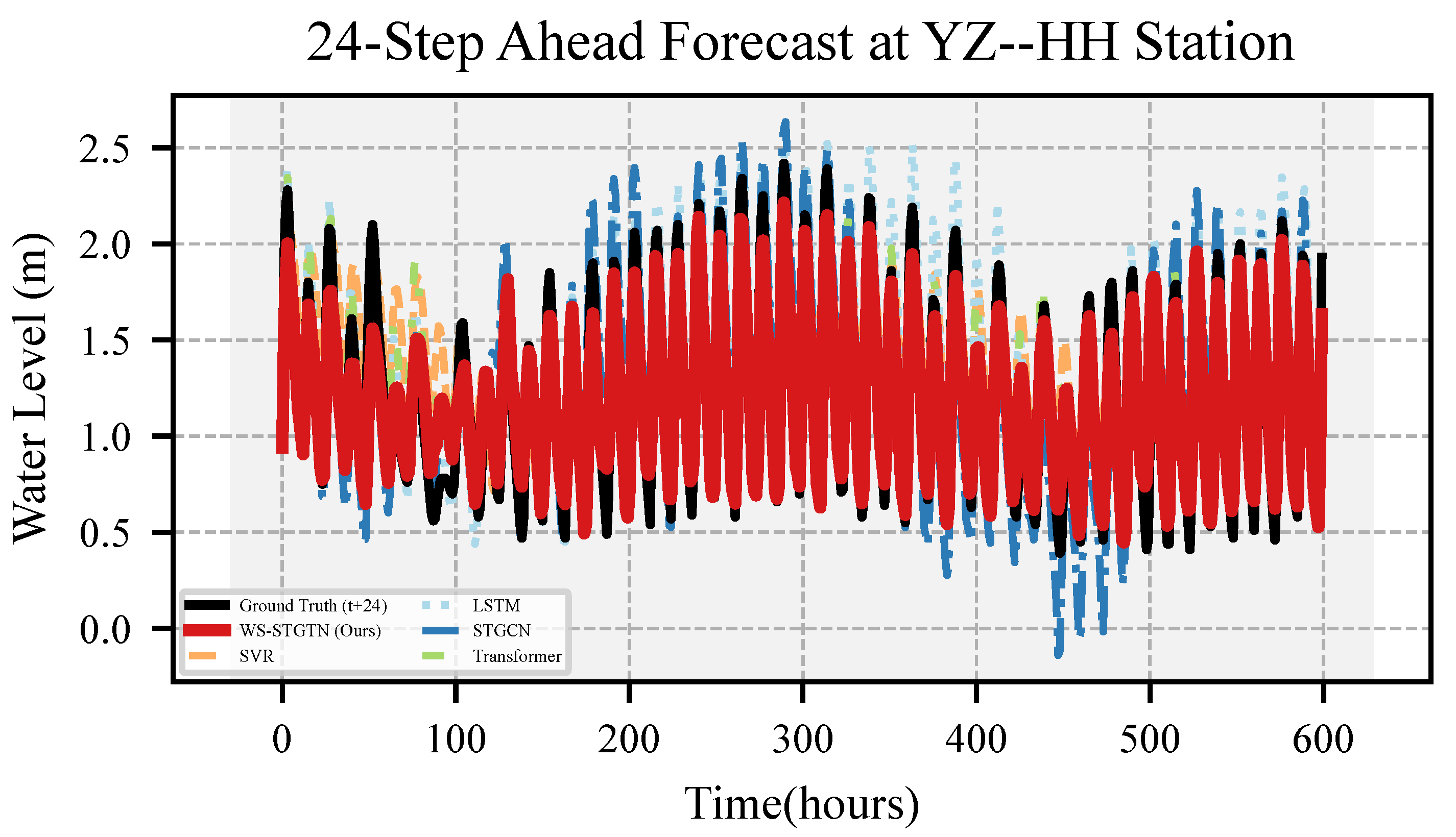
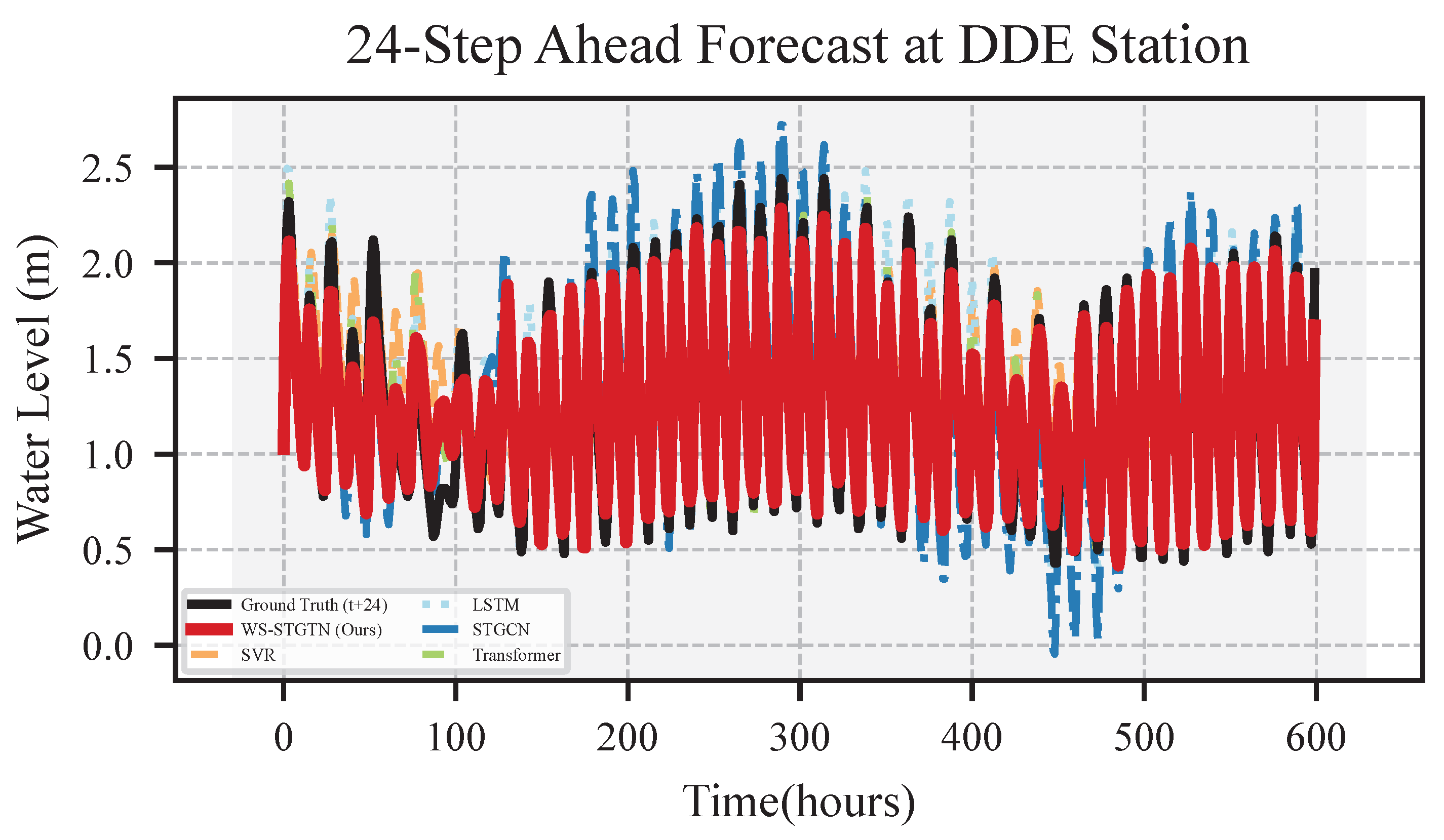
Figure 7, Figure 8, Figure 9, Figure 10 and Figure 11 present the 24-step ahead predictions conducted by WS-STGTN and the baseline models (SVR, LSTM, STGCN, Transformer), alongside the corresponding ground truth, for all five water level datasets. Here, each time step corresponds to 1 h, meaning that the 24-step ahead predictions cover a total of 24 h.

Each figure illustrates that the trend lines of the predictions generated by WS-STGTN closely align with the respective ground truth trends across all datasets. This high degree of similarity is consistently observed, even during periods of significant water level fluctuation.

In contrast, the forecasting performance of the baseline models reveals a notable lag across all datasets, suggesting that error accumulation significantly impacts their accuracy and stability, particularly in multi-step long-term predictions.

Overall, WS-STGTN demonstrates a more accurate and reliable fitted trend on all five real-world datasets compared to the baselines, effectively capturing both the overall trend and local variations in water level.

5.4. Ablation Study

We conduct ablation studies to investigate the contribution of each component of WS-STGTN: temporal DTW-based similarity in graph construction, weighted MSE, graph attention, and temporal self-attention.

Table 4. Ablation study of WS-STGTN across five Yangtze River water level datasets.

Dataset	Model Variant	MSE				MAPE
		1–8	9–16	17–24	1–24	1–8	9–16	17–24	1–24
	NoDTW	$6.87\times {10}^{-2}$	$8.40\times {10}^{-2}$	$9.03\times {10}^{-2}$	$8.10\times {10}^{-2}$	11.65	12.18	12.93	12.25
	NoWMSE	$4.73\times {10}^{-2}$	$6.03\times {10}^{-2}$	$8.50\times {10}^{-2}$	$6.42\times {10}^{-2}$	7.99	9.65	11.57	9.74
XS–HH	NoGAT	$4.94\times {10}^{-2}$	$6.10\times {10}^{-2}$	$6.62\times {10}^{-2}$	$5.89\times {10}^{-2}$	8.04	9.69	10.50	9.41
	NoTimeAttn	$5.28\times {10}^{-2}$	$7.53\times {10}^{-2}$	$1.08\times {10}^{-1}$	$7.86\times {10}^{-2}$	9.09	10.96	12.95	11.00
	WS-STGTN	$\mathbf{4}.\mathbf{42}\times {\mathbf{10}}^{-\mathbf{2}}$	$\mathbf{5}.\mathbf{73}\times {\mathbf{10}}^{-\mathbf{2}}$	$\mathbf{6}.\mathbf{51}\times {\mathbf{10}}^{-\mathbf{2}}$	$\mathbf{5}.\mathbf{55}\times {\mathbf{10}}^{-\mathbf{2}}$	6.99	8.76	9.50	8.42
	NoDTW	$3.56\times {10}^{-2}$	$5.11\times {10}^{-2}$	$5.26\times {10}^{-2}$	$4.64\times {10}^{-2}$	9.41	11.55	11.99	10.98
	NoWMSE	$1.43\times {10}^{-2}$	$2.12\times {10}^{-2}$	$2.63\times {10}^{-2}$	$2.06\times {10}^{-2}$	6.86	8.68	9.96	8.50
QJ	NoGAT	$1.62\times {10}^{-2}$	$2.35\times {10}^{-2}$	$2.63\times {10}^{-2}$	$2.20\times {10}^{-2}$	7.05	8.70	9.29	8.35
	NoTimeAttn	$1.72\times {10}^{-2}$	$2.42\times {10}^{-2}$	$2.89\times {10}^{-2}$	$2.34\times {10}^{-2}$	8.05	9.77	10.79	9.54
	WS-STGTN	$\mathbf{1}.\mathbf{24}\times {\mathbf{10}}^{-\mathbf{2}}$	$\mathbf{2}.\mathbf{04}\times {\mathbf{10}}^{-\mathbf{2}}$	$\mathbf{2}.\mathbf{44}\times {\mathbf{10}}^{-\mathbf{2}}$	$\mathbf{1}.\mathbf{91}\times {\mathbf{10}}^{-\mathbf{2}}$	5.80	7.87	8.68	7.45
	NoDTW	$3.33\times {10}^{-2}$	$4.30\times {10}^{-2}$	$4.63\times {10}^{-2}$	$4.09\times {10}^{-2}$	10.15	11.40	11.98	11.18
	NoWMSE	$1.80\times {10}^{-2}$	$2.43\times {10}^{-2}$	$2.91\times {10}^{-2}$	$2.38\times {10}^{-2}$	8.77	10.29	11.60	10.22
SJK	NoGAT	$1.78\times {10}^{-2}$	$2.48\times {10}^{-2}$	$2.73\times {10}^{-2}$	$2.33\times {10}^{-2}$	8.16	9.78	10.27	9.40
	NoTimeAttn	$2.02\times {10}^{-2}$	$2.77\times {10}^{-2}$	$3.25\times {10}^{-2}$	$2.68\times {10}^{-2}$	9.56	11.47	12.52	11.18
	WS-STGTN	$\mathbf{1}.\mathbf{43}\times {\mathbf{10}}^{-\mathbf{2}}$	$\mathbf{2}.\mathbf{18}\times {\mathbf{10}}^{-\mathbf{2}}$	$\mathbf{2}.\mathbf{56}\times {\mathbf{10}}^{-\mathbf{2}}$	$\mathbf{2}.\mathbf{06}\times {\mathbf{10}}^{-\mathbf{2}}$	7.04	8.91	9.54	8.49
	NoDTW	$3.78\times {10}^{-2}$	$4.91\times {10}^{-2}$	$5.75\times {10}^{-2}$	$4.82\times {10}^{-2}$	11.32	13.44	15.20	13.32
	NoWMSE	$1.71\times {10}^{-2}$	$2.41\times {10}^{-2}$	$3.02\times {10}^{-2}$	$2.38\times {10}^{-2}$	8.75	11.04	12.97	10.92
YZ–HH	NoGAT	$1.98\times {10}^{-2}$	$2.79\times {10}^{-2}$	$3.08\times {10}^{-2}$	$2.62\times {10}^{-2}$	9.22	11.40	12.31	10.98
	NoTimeAttn	$2.12\times {10}^{-2}$	$2.87\times {10}^{-2}$	$3.40\times {10}^{-2}$	$2.80\times {10}^{-2}$	10.94	13.65	14.92	13.17
	WS-STGTN	$\mathbf{1}.\mathbf{56}\times {\mathbf{10}}^{-\mathbf{2}}$	$\mathbf{2}.\mathbf{37}\times {\mathbf{10}}^{-\mathbf{2}}$	$\mathbf{2}.\mathbf{87}\times {\mathbf{10}}^{-\mathbf{2}}$	$\mathbf{2}.\mathbf{27}\times {\mathbf{10}}^{-\mathbf{2}}$	7.58	9.97	11.14	9.57
	NoDTW	$3.73\times {10}^{-2}$	$4.65\times {10}^{-2}$	$5.15\times {10}^{-2}$	$4.51\times {10}^{-2}$	11.29	12.94	14.16	12.79
	NoWMSE	$2.05\times {10}^{-2}$	$2.79\times {10}^{-2}$	$3.31\times {10}^{-2}$	$2.72\times {10}^{-2}$	9.30	11.42	13.00	11.24
DDE	NoGAT	$2.27\times {10}^{-2}$	$3.10\times {10}^{-2}$	$3.35\times {10}^{-2}$	$2.91\times {10}^{-2}$	8.91	10.87	11.63	10.47
	NoTimeAttn	$2.52\times {10}^{-2}$	$3.36\times {10}^{-2}$	$3.84\times {10}^{-2}$	$3.24\times {10}^{-2}$	11.34	13.50	14.76	13.20
	WS-STGTN	$\mathbf{1}.\mathbf{83}\times {\mathbf{10}}^{-\mathbf{2}}$	$\mathbf{2}.\mathbf{72}\times {\mathbf{10}}^{-\mathbf{2}}$	$\mathbf{3}.\mathbf{10}\times {\mathbf{10}}^{-\mathbf{2}}$	$\mathbf{2}.\mathbf{55}\times {\mathbf{10}}^{-\mathbf{2}}$	7.75	9.93	10.74	9.47

shows results on the XS–HH dataset. Each variant reflects a realistic modeling scenario: NoDTW ignores temporal misalignment such as flow lag; NoWMSE omits prioritization of critical hydrological events; NoGAT replaces graph attention with convolution, mimicking static spatial aggregation; and NoTimeAttn substitutes temporal self-attention with LSTM, reflecting sequence-based modeling without global context. These variants isolate the contribution of each component under real-world forecasting conditions.

5.5. Forecasting Performance Comparison

Table 2 summarizes multi-horizon results (short: $1–8$, medium: $9–16$, long: $17–24$, and overall: $1–24$) on five Yangtze River water-level datasets (XS–HH, QJ, SJK, YZ–HH, DDE). Across all datasets and horizons, WS-STGTN consistently outperforms SVR, LSTM, STGCN, and Transformer in both MSE and MAPE.

On the full $1–24$ horizon, WS-STGTN reduces errors relative to the Transformer by approximately 28% in MSE 21%in MAPE on average, reflecting robust gains over a strong sequence model with global attention. Dataset-wise, improvements range from modest to large; the biggest benefits appear on SJK and YZ–HH, e.g., on YZ–HH ($1–24$) WS-STGTN attains roughly $40\%$ MSE and $35\%$ MAPE versus the Transformer. Compared with LSTM, the average gains are about one-third on both metrics, underscoring the value of explicitly modeling spatiotemporal dependencies and lag-aware inter-station relations beyond sequence-only architectures.

Across horizons, improvements are stable and most pronounced at short and medium ranges: averaged over datasets, WS-STGTN lowers short-term ($1–8$) MSE by about $38\%$ relative to the Transformer, while long-range ($17–24$) forecasts still benefit notably. Relative to the graph-based STGCN, WS-STGTN secures clear additional gains, highlighting the advantages of lag-aware graph construction and dual (graph and temporal) attention over static convolutional aggregation; against classical SVR, margins are, as expected, very large. In aggregate, WS-STGTN achieves state-of-the-art performance across datasets and horizons, and the combination of DTW-driven, lag-aware graph construction with graph attention and temporal self-attention translates into robust, accurate multi-step water-level forecasting.

6. Conclusions

Accurate water level prediction is vital for ensuring navigational safety and optimizing the economic benefits of waterways. However, conventional forecasting models often fall short due to their inability to adequately model the complex and dynamic spatiotemporal relationships within river networks. In this paper, we proposed the Water State-aware Spatiotemporal Graph Transformer Network (WS-STGTN), a novel deep learning framework designed to overcome these limitations.

The core strengths of WS-STGTN lie in its two primary innovations: a dual-weight graph construction that fuses static geographical information with dynamic temporal correlations derived from DTW, and a state-aware weighted loss function that prioritizes forecast accuracy during critical high and low water level events.

Through extensive experiments on five real-world Yangtze River datasets (XS–HH, QJ, SJK, YZ–HH, DDE), WS-STGTN consistently outperformed representative baselines, including SVR, LSTM, STGCN, and Transformer. On the full 1–24-step horizon, WS-STGTN achieved an average reduction in MSE of 27.6% and an average improvement in Accuracy (derived from MAPE) of 21.1% relative to Transformer. Compared with LSTM, average improvements were 37% in MSE and 35% in Accuracy. Dataset-specific gains were especially notable for YZ–HH and SJK, where MSE reductions exceeded 40% and Accuracy improved by over 30%. In addition, WS-STGTN achieved the highest coefficient of determination ($R^2$) across all datasets, averaging around 0.95–0.97, which is higher than Transformer (0.93–0.94) and LSTM (0.92–0.93), demonstrating its stronger capability to explain observed water-level variance. These results quantitatively confirm the advantage of combining DTW-driven lag-aware graph construction with graph and temporal attention mechanisms. The results underscore the significant value of explicitly modeling the underlying hydrological connectivity and focusing on state-sensitive errors for robust and reliable water level forecasting.

6.1. Limitations

Despite its promising performance, this study has several limitations. The graph structure, while dynamic through DTW-based weighting, relies on a fixed set of monitoring stations and does not inherently account for sudden topological changes, such as the emergence of new tributaries or man-made alterations to the waterway. In real-world hydrological environments, the graph can be updated periodically or in an online manner by recalculating inter-station relationships within a recent time window, enabling WS-STGTN to adapt to evolving flow patterns and connectivity. Future work could explore incremental or event-driven graph updates to ensure real-time adaptability, addressing a limitation present in traditional graph-based or sequence-only models. Furthermore, the definition of water level states via k-means clustering is entirely data-driven and unsupervised; incorporating domain-specific hydrological thresholds could provide more operationally relevant state definitions. While adaptive graph updates may introduce additional computational overhead, this cost can be mitigated through sparse updates or asynchronous recalibration, as partially discussed in the experiments. Compared with previous approaches, WS-STGTN balances predictive accuracy and adaptability, offering a systematic improvement over static or purely sequential forecasting methods. Lastly, the model’s complexity, while advantageous for capturing spatiotemporal dependencies, may require substantial computational resources for training and inference, potentially limiting deployment in resource-constrained settings.

6.2. Future Work

Future research could extend this work in several promising directions. First, incorporating a wider range of exogenous variables, such as rainfall from weather station and tidal information, could significantly enhance predictive accuracy. Second, exploring methods for dynamic graph evolution, where nodes and edges can be added or removed over time, would improve the model’s adaptability to long-term changes in the river system. Finally, developing a lightweight version of WS-STGTN or employing model compression techniques could facilitate its practical application in real-time, on-board vessel navigation systems.