A New Collision Risk Assessment Algorithm Based on Ship’s Finite-Time Reachable Set

Abstract

Collision risk assessment is essential for navigators or automatic navigation systems to identify potential risks in specific encounter scenarios and to make informed decisions regarding subsequent collision avoidance measures. This paper proposes a quantitative ship collision risk assessment algorithm based on the reachability of the vessels. The concept of a ship’s finite-time reachable set is introduced to characterize spatial area accessible to the vessel within the navigator’s “action time”. A novel risk assessment algorithm is proposed that takes into account not only the probability of collision but also the anticipated consequences. Compared to previous risk assessment methodologies, this new quantitative assessment algorithm can provide both upper and lower bounds of ongoing collision risk according to the real-time motion characteristics of ships. The effectiveness of the new risk assessment algorithm is examined by simulation studies that cover three typical encounter situations: head-on, crossing, and overtaking. The results show that our risk assessment algorithm can accurately predict the trend of risk variation.

1. Introduction

Maritime collisions are some of the most complex and costly incidents that can occur at sea. According to the Global Integrated Shipping Information System (GISIS) database, which provides a comprehensive repository of data on maritime accidents reported to the International Maritime Organization (IMO), ship collision accidents account for approximately 20% of all maritime accident categories. When examining the temporal period from 2005 to 2017, the database documents a total of 936 vessel collisions, representing nearly 25% of all recorded maritime accidents [1]. Over the past decade, the number of maritime collision accidents has shown a declining trend. However, a recent collision in the North Sea has once again highlighted the critical importance of collision avoidance in maritime shipping. On 10 March 2025, the Portugal-flagged cargo ship Solong collided with a U.S.-flagged oil tanker while the latter was anchored in the North Sea, off the eastern coast of England, resulting in both vessels catching fire [2]. This accident further reminds us that ship collision avoidance continues to face significant challenges.

Numerous studies indicate that both direct and indirect human errors are predominant contributors to maritime collisions [3,4]. To enhance the quality and efficacy of navigational safety, computer-aided navigation systems have been developed, which can integrate the information from various sensors, including radar systems, Automatic Identification Systems (AIS), Electronic Chart Display and Information Systems (ECDIS), among others [5]. Recent advancements in machine vision, information fusion, and intelligent decision-making have enabled advanced algorithms to effectively utilize information from these sensors to assist ship navigators in monitoring situations, assessing navigation risks, and operating vessels, thereby mitigating human errors. Collision risk assessment, as a crucial component of computer-aided navigation systems, employs a quantitative framework to estimate navigational risks using various perception data, providing valuable reference for collision avoidance decisions.

Tremendous efforts have been made to obtain a proper collision risk assessment in the literature. Generally, techniques for collision risk assessment fall primarily into two categories. The first is qualitative risk assessment methods, which focus on the identification and characterization of potential collision events. In other words, these approaches fundamentally involve the construction of a conditional framework intended to determine the incidence of impending collisions. One widely used two-dimensional assessment method is based on the concept of ship domain (SD). SD defines “a two-dimensional area surrounding a ship which other ships must avoid” so that any target ship (TS) enters the SD of the own ship (OS) indicates a potential collision risk. SD-based methods are originally introduced to analyze the waterway capacity [6] and subsequently used to evaluate ship collision risk [7,8,9]. Its core idea is to make a qualitative judgment based on whether a TS enters the defined SD. Therefore, the most SD-based collision risk assessment methods concentrate on developing the geometric configuration of the domain model. Several excellent reviews in the literature extensively cover the basic concepts of SD models and their practical applications [7,8,9], and the reader is referred in particular to those by Li, Cheng, and coworkers [9]. Although SD-based qualitative risk assessment methods have obtained considerable academic interest primarily due to their simplicity and robustness, SD-based risk assessment methods inherently fail to capture dynamic risk variations, since the evaluated risk only changes when a TS enters the SD of OS or sails away from the inside. Some studies have employed the distance between domains [10] and the size of their intersection areas [11] as a metric for quantitative risk assessment based on SD models, yet these studies fail to address scenarios involving complete domain coverage.

On the other hand, the distance between two vessels has been used as a primary metric of collision risk and has consistently been employed in quantitative collision risk assessment, since two vessels collide if and only if they come into contact, in other words, their spatial distance is zero. Thus, the Closest Point of Approach (CPA) represents the critical position whereby the own ship and the target ship (this is regarded as the most dangerous ship among those near the own ship) are the closest, assuming the current heading angle and speed are maintained [12,13]. Two essential metrics derived from this concept are Distance to CPA (DCPA) and Time to CPA (TCPA). DCPA and TCPA are widely recognized as key parameters and are integrated into most modern Radar and ECDIS, providing navigators with valuable risk estimation capabilities. DCPA offers a direct indication of the minimum distance at the most critical moment for both vessels, while TCPA provides immediate insight into the urgency level faced by both vessels, allowing for appropriate timing of collision avoidance maneuvers [13]. However, some studies report that they may become ineffective in some specific situations [8,10,11].

Many risk assessment methods, such as COLREG-based methods [14], encounter situation recognition methods [15], and spatial–temporal analysis methods [16] are also proposed to provide a quantitative risk assessment. Recent developments in artificial intelligence have significantly contributed to maritime vessel collision risk assessment [17] introduces a novel collision risk index (NCRI) that incorporates the International Regulations for Collision Avoidance at Sea (COLREGs), establishing a Fuzzy Dynamic Elliptical Ship Domain (F-DESD) with dynamical boundaries calibrated according to vessel dimensions, velocity, maneuverability, and navigator experience [18] proposes a comprehensive index termed enhanced collision risk index with weather (ECRI-W), employing fuzzy logic to integrate collision risk index (CRI) with resultant environmental factor indices. A regional vessel collision risk prediction framework utilizing encoder–decoder LSTM neural networks, as presented in [19], facilitates collision risk prediction. The convolutional neural networks (CNN) encoder is implemented to capture spatial risk features and compress the collision risk structure scale. The authors in [20] developed a quantitative risk analysis methodology based on complex networks and decision-making trial and evaluation laboratory (DEMATEL) to investigate the evolution of ship collision accidents. By treating collision avoidance procedure as a static game with incomplete information, a predictive model for collision avoidance intentions was developed by taking account into risk attitude probabilities in [21]. Ref. [22] establishes a novel fault tree analysis–fuzzy Bayesian network (FTA-FBN) framework to conduct collision risk assessment of Maritime Autonomous Surface Ships (MASS) under conditions of data uncertainty. Although these AI-driven approaches to ship collision risk assessment have achieved notable success in specific applications, the development of corresponding models necessitates extensive training datasets. Additionally, these models encounter challenges such as poor interpretability and difficulty in maintaining stability.

Besides the area of ship collision risk assessment, the safety potential field (SPF) method quantifies driving risks originating from artificial potential field (APF) theory, which is a modeling approach to quantify the risks associated with spatial proximity between objects and is extensively used in land vehicle driving risk assessment [23,24,25,26]. APF-based risk descriptions are usually used as the constraints for collision avoidance algorithms, such as model predictive control (MPC) algorithms [27,28,29] and the minimum navigation risk algorithm [30]. Ref. [31] compared the APF method with the collision risk index (CRI) method and safe zone method in the free-running tests of unmanned surface vehicles (USVs). Although these field-based models can provide quantitative risk assessment, they rely on the assumption that repulsive forces exist between objects. However, such repulsive forces are insufficiently strong to influence the motion of macroscopic objects. These field-based models reflect considerable subjective interpretation rather than objective physical phenomena.

Actually, the collision occurs if and only if the subjects reach the same spatial place simultaneously. Thus, the reachability should be considered in the assessment of collision risk. Reachability is a fundamental concept in control theory, with the notion of reachable sets introduced in the 1960s as a method for bounding within this domain. A reachable set encompasses the collection of all states that can be attained at a given time from an initial state by exploring all control inputs within a defined control constraint set [32]. The introduction of reachable sets has garnered significant interest among researchers. Numerous scholars have investigated computational methods for reachable sets, proposing various solution approaches. Ref. [33] uses the concept of the reachability to analyze the safety of hybrid systems. Zhou C proposed a reachability analysis method based on level set approaches, utilizing Hamilton–Jacobi partial differential equations to solve for reachable sets, which subsequently informed the development of maneuvering strategies based on safety envelopes [34,35]. Manzinger and coauthors in [36] combined reachable sets with convex optimization techniques to propose a novel motion planning method for autonomous vehicles, effectively addressing the computational burden associated with this problem. Ref. [37] developed a formal safety verification method based on analytic probabilistic reachability computation, which can estimate the probability of controlled non-deterministic systems entering unsafe states subject to disturbances. Ref. [38] proposed a ship dynamic collision avoidance algorithm based on a reachable set so that the reachability of ships could be taken into account for collision avoidance. Similar concepts have been applied to the collision avoidance challenge in maritime navigation, such as [28,39], which utilize MPC algorithms to generate viable navigational trajectories. These studies indicate that the reachability of a dynamic system is closely associated with both motion and safety, which are also fundamental factors in the comprehensive assessment of ship navigational risk. Particularly, the requirement that vessels reach the same location simultaneously as an essential condition for collision implies that the point of impact must inevitably be located within the reachable range of both vessels, as defined by their respective reachable sets. Additionally, one must take into account the impact of temporal considerations, influenced by the operators’ experiential judgment and the inertia characteristics of vessels, on the vessels’ accessible range.

Therefore, this paper introduces the concept of a ship’s finite-time reachable set to establish a connection between collision risk and the reachability of ships, thereby enabling comprehensive risk evaluation across all feasible trajectories that the vessel can navigate through. Conceptually, the ship’s finite-time reachable set is defined as a region in two-dimensional space that illustrates the reachable area of the vessel within that specified time period. This set is constituted by all the trajectories that the vessel can go along. In other words, it facilitates the prediction of all feasible positions through which the ship may navigate during the given time period. Simultaneously, the vessel’s dynamics are employed to derive the finite-time reachable set so that the ship’s current states, relevant environmental influences, and the permissible actions of the navigator can be taken into account for the collision risk assessment. Thus, the ship’s finite-time reachable set also encompasses all future states into which the ship’s trajectories may evolve for any given initial states. Moreover, the finite-time reachable set can also take the reaction time of the navigator into account by selecting the temporal duration for this set to be covered, thereby reflecting the navigator’s experience. From a navigational risk assessment perspective, the area of a ship’s finite-time reachable set is compatible with conventional ship domains, since collision will not occur if no obstacles exist within its reachable set. Furthermore, regions accessible to both vessels inherently possess heightened collision probability. Consequently, the intersection area between the finite-time reachable sets of both vessels can be employed as a quantitative measure to quantify the collision probability. Similar to [10,11], the ratio of the overlapping region’s area to the area of the ship’s finite-time reachable set can serve as a geometric probability metric for collision occurrence. Therefore, the probability of collision occurrence is directly proportional to the size of the overlapping region. In addition to its compatibility, another advantage of the ship’s finite-time reach-able set is that it is characterized by all trajectories of both vessels. This enables the prediction of all potential collisions in the overlapping region and facilitates more comprehensive risk analysis. According to [40,41,42], the collision risk assessment needs to consider both the probability and the consequences related to the collision. The consequences related to potential collisions in the overlapping region can be modeled by the impact force, as the corresponding vessel states can be obtained at every location within the overlapping region, thereby enabling impact force estimation using the model employed in [10,11]. Compared to the previous research on collision risk assessment reviewed in [27,28,29], this method can provide both upper and lower bounds of collision risk, since the minimum and maximum values of the consequences can be calculated. This enables navigators to ascertain the range of navigational risk prior to making collision avoidance decisions. Simulation studies show that our collision risk assessment method is effective. The evaluated risk is also continuous with respect to time so that the trend of the risk variation can be clearly exhibited.

In summary, the main contribution of our work can be outlined as follows:

• A novel collision risk assessment model is developed based on an innovative reachability characterization—the ship’s finite-time reachable set—which effectively captures the reachability of both the own ship and the target ship, along with temporal consideration.
• The proposed risk assessment framework not only enables quantitative evaluation of collision risk but also provides its comprehensive boundary for the first time, so that it makes the model more logical and interpretable, while furnishing navigators with enhanced information for collision avoidance decision-making.
• Compared to the previous research on collision risk assessment, our risk assessment algorithm can provide a more rational interpretation and prediction of the variations and trends in risk according to the real-time motion characteristics of ships.

The remainder of the paper is organized as follows. Section 2 addresses the problem of quantitative collision risk assessment, and the requirements of risk assessment are also given. Section 3 introduces the concept of ship’s finite-time reachable set. The risk assessment algorithm based on the ship’s finite-time reachable set is proposed in Section 4. Simulations are conducted in Section 5. Finally, Section 6 presents conclusion.

2. Problem Formulation of Ship Navigation Risk Assessment

Risk assessment aims to find the relationship between collision risk and multiple contributing factors, including vessel maneuverability, kinematic situations, and environmental influences. Particularly, risk can be quantified through an evaluation function $F_{\mathrm{R}}$ that incorporates these multifaceted parameters to produce a comprehensive assessment metric

$$R_{\mathrm{own}}=F_R(X)$$

(1)

where $R_{\mathrm{own}}\in R$ denotes the risk of OS, and X is a vector that includes all the factors related to the risk. For instance, the risk evaluation function of conventional SD-based risk assessment methodologies can be mathematically expressed as

$$R_{o,k}=F_R(X)=F_R(P_t^k)=\left\{\begin{array}{l}1,\hspace{1em}{P}_t^k\in D_{own}\\ 0,\hspace{1em}{P}_t^k\notin D_{own}\end{array}\right.$$

(2)

where $D_{own}$ denotes the ship domain of OS, $R_{o,k}$ denotes the risk of OS with respect to the k-th TS, and $P_t^k$ is the position of the k-th TS. Typically, $D_{own}$ could be a two-dimensional region around OS. Thus, the ship domain of OS can be defined by its boundary points, i.e.,

$$\partial D_{own}(x_o,y_o)=\left\{(x_{o_i},y_{o_i}),i=1,\dots ,n_o\right\}$$

(3)

and for the k-th TS, its ship domain can be defined as

$$\partial D_t^k(x_t^k,y_t^k)=\left\{(x_{t_i}^k,y_{t_i}^k),i=1,\dots ,n_t^k\right\}$$

(4)

where $\partial$ denotes the boundary of a region, and $(x_o,y_o)$ and $(x_t^k,y_t^k)$ are the reference coordinates of the OS and the k-th TS, respectively (they are usually the coordinates of the center of mass); $(x_{o_i},y_{o_i}),1,\dots ,n_o$ and $(x_{t_i}^k,y_{t_i}^k),1,\dots ,n_k$ are the coordinates of the points on their boundaries, respectively.

Equation (2) is a discontinuous function with respect to the position of the k-th TS, which also indicates that the conversional SD-based risk assessment algorithms only take $P_t^k$ and $D_{own}$ into consideration. While numerous factors contribute to vessel collision scenarios, it is methodologically sound to evaluate risk primarily based on the relative kinematic relationships between vessels, data readily extractable from AIS transmissions from TSes.

Collision risk assessment conventionally entails estimating the potential hazard to involved entities assuming their current states remain unaltered. However, significant uncertainty characterizes the kinematic profiles of both OS and TS, as both vessels possess the capacity to modify their navigational parameters and motion trajectories. Therefore, such uncertainty must be incorporated into the collision risk evaluation function $F_{\mathrm{R}}(\cdot )$. It implies that the maneuverability of both OS and TS should be considered in the modeling of $F_{\mathrm{R}}(\cdot )$. Furthermore, collision risk assessment should incorporate a degree of foresight, thereby providing navigators or vessel navigation systems with adequate time to adjust the vessel’s status for collision avoidance. On the other hand, a continuous mathematical model of collision risk between OS and TS offers dual advantages: it enables precise determination of current collision risk while simultaneously facilitating trend analysis. Consequently, the collision risk assessment framework proposed in this paper concentrates on risk quantification through the development of a continuous evaluation function that satisfies the following criteria:

(R₁) $F_{\mathrm{R}}(\cdot )$ only depends on the current states and parameters of OS and TS.

(R₂) $F_{\mathrm{R}}(\cdot )$ is continuous.

3. Ship’s Finite-Time Reachable Set for Navigation Risk Assessment

A collision between two ships usually refers to two things that occur simultaneously, one of which is physical contact between the two vessels and the other is that the energy released after contact damages the vessels. Therefore, a fundamental prerequisite for a ship collision is that at least one ship must lie within the reachable area of the other; otherwise, physical contact will not occur, and subsequent collision will be precluded. Understanding the reachable area of a vessel is essential for conducting a collision risk assessment. The concepts of a ship’s reachable set and its simplified reachable set are introduced in the following sections to delineate the region accessible to the vessel.

3.1. Reachability and Reachable Set

In the field of control systems engineering, reachability is a fundamental concept that describes where the state of a computational system with a set of allowed input can reach from a given initial condition. Generally, the reachable set of a system usually means the set of all states that can be reached along trajectories from the specified initial condition. If one can accurately determine the set of states from which a system may inadvertently step or be pushed into an unsafe configuration, then system safety can be verified by ensuring that the system state remains outside of this set. Typically, a dynamical system $\sum$ can be written as

$$\sum :\dot{x}=f(x,u,t)$$

(5)

where x is an n-vector representing the state of the system $\sum$; u is an m-vector representing the input to the system. The space of inputs is the function space $L_p(t_0,t_1)$ for various values of p, $1\le p\le \infty$ and arbitrary finite intervals of time $(t_0,t_1)$. Thus, for a given problem, every admissible input u(t) must satisfy the relation

$$u\in U\subset L_p(t_0,t_1)$$

(6)

for some value of p and some set U. The reachable state and the reachable set of the system can be defined as follows [32].

Definition 1 (Reachable state).

Consider the system $\sum$ with initial state $x(t_0)=x_0$ and admissible controls which satisfy relation Equation (6) on every finite time interval $(t_0,t_1)$ for a given control set U. The state $x_1\in E^n$ is said to be reachable at time $t_1$ from $x(t_0)=x_0$ if there exists an admissible control and a time $t_1\ge t_0$ such that the corresponding solution of Equation (5) at time $t_1$ coincides with $x_1$.

Definition 2 (Reachable set).

The reachable set $R(t_1;x_0)\subset E^n$ at time $t_1$ for the system $\sum$ with control constraint set U is defined as the set of all states $x\in E^n$ reachable at time $t_1$ from $x(t_0)=x_0$ by admissible controls.

According to the above definitions, the reachable set can reflect the range that the states cover in a certain time. Moreover, the reachable set closely depends on the dynamics of the system, the control input, the initial condition and the time interval so that the reach-able set contains the essential features of the system. Thus, different systems will have different reachable sets.

In order to illustrate the reachable set of a dynamic system, we show the reachable sets of a car. The motion of a car can be modeled as [30]

$${\Sigma }_c:\left\{\begin{array}{c}\dot{x}=\omega \cos \theta \\ \dot{y}=\omega \sin \theta \\ \dot{\theta }=u\end{array}\right.$$

(7)

where the variables x, y specify the center mass position in the two-dimensional plane; $\theta$ is the angle between the direction of the velocity vector and that of the vertical axis y measured clockwise from the latter. Control u changes the angular velocity; control $\omega$ is responsible for instantaneous changes in the linear velocity magnitude. It is natural to consider control dynamics where the control u is from the interval [−1, 1] and $\omega$ is from the interval [a, 1]. If a = 1, Dubins’ car model is obtained; if a = −1, Reeds and Shepp’s car model appears. Figure 1 shows the reachable sets of a Dubins’ car model in 1 s. $\omega$ in Figure 1a is 0.5, and in Figure 1b is 1.0. The reachable sets are illustrated in 3D space. The solid line and the dashed line show the boundaries of the reachable sets. If we only focus on the range where the car can reach, we actually only need to focus on the projection of the reachable set on the X-Y plane. The projection area of Figure 1b is larger than that of Figure 1a since ω of the model in Figure 1b is also greater than in Figure 1a. Moreover, the size of the entire reachable set should be much larger than the simulations, if the simulation time is not limited.

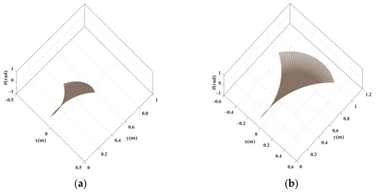
Figure 1. The reachable set of a Dubins’ car model in 1 s. (a) ω = 0.5; (b) ω = 1.0.

3.2. Ship’s Finite-Time Reachable Set

The reachability of a ship is an important consideration of risk assessment since collision will not happen if own ship cannot reach any obstacles. Thus, the ship’s reachable set can be used to model the safe domain.

According to Definition 1 and 2, the ship’s reachable set depends on its dynamics, which is usually expressed by a motion model. In particular, the maneuvering modeling group (MMG) model, which is one of the solutions for ship maneuvering predictions [31], is a second-order response maneuver model and can be used to obtain the ship’s reachable set. The MMG ship motion model could be described as follows:

$${\Sigma }_s:\left\{\begin{array}{cc}\hfill \dot{x}=& u\cos \psi -v\sin \psi \hfill \\ \hfill \dot{y}=& u\sin \psi +v\cos \psi \hfill \\ \hfill \dot{\psi }=& r\hfill \\ \hfill (m+m_x)\dot{u}-(m+m_x)vr=& X_H+X_P+X_R\hfill \\ \hfill (m+m_y)\dot{v}+(m+m_x)ur=& Y_H+Y_P+Y_R\hfill \\ \hfill (I_{zz}+J_{zz})\dot{r}=& N_H+N_P+N_R\hfill \end{array}\right.$$

(8)

where

x and y are the coordinates in the earth-fixed frame, respectively.

m and I_zz are mass and moment of inertia of the ship, respectively.

m_x, m_y and J_zz denote added mass in the x- and y-directions and added moment of inertia about z-axis, respectively.

X, Y and N denote surge forces, sway forces and yaw moments, respectively, due to hydrodynamics, propeller and rudder denoted by subscripts H, P and R.

u and v are the velocities along X (towards forward) and Y axes (towards starboard), respectively.

$\psi$ and r are the yaw angle and its rotational rate, respectively.

$X_{H,P,R}$, $Y_{H,P,R}$ and $N_{H,P,R}$ are the driven forces and can usually be regulated by operating the actuators like the shaft revolution $\omega$ of the propeller and the rudder angle $\delta$. ${\Sigma }_s$ can be simply represented as

$${\Sigma }_s:{\dot{X}}_s=F_s(X_s,U)$$

(9)

where $X_s$ is the vector of all ship states, i.e., $X_s={[x\hspace{0.33em}y\hspace{0.33em}\psi \hspace{0.33em}u\hspace{0.33em}v\hspace{0.33em}r]}^T$, $U$ is the vector of the ship’s control inputs, i.e., $U={[\omega \hspace{0.33em}\delta ]}^T$.

According to the definition of the reachable set, the ship’s reachable set can be defined as follows

$$R{S}_s(t_1,X_s)=\left\{X_s\left|{\dot{X}}_s=F_s(X_s,U),X_s(t_0)=X_{s0},t\in [t_0,t_1],U\right.\in U_s\right\}$$

(10)

where $X_{s0}$ is the initial state of ${\sum }_s$, and $U_s$ is the set that contains all admissible control inputs. Usually, $U_s$ is related to the operation range of the actuators, i.e.,

$$U_s=\left\{(\omega ,\delta )\left|\omega \right.\in \left[{\omega }_{\min },{\omega }_{\max }\right],\delta \in \left[{\delta }_{\min },{\delta }_{\max }\right]\right\}$$

(11)

Moreover, our focus centers on the potential destinations a vessel can achieve when contemplating the ship’s reachability. Practically, the ship’s reachable set can be redefined as

$${\overline{RS}}_s(t_1,x_s)=\left\{x_s\left|{\dot{X}}_s=F_s(X_s,U),X_s(t_0)=X_{s0},x_s={[x\hspace{0.33em}y]}^T,t\in [t_0,t_1],U\right.\in U_s\right\}$$

(12)

Obviously, the comprehensive exploration of the entire input space and time t₁ to ascertain the entirety of ${\overline{RS}}_s(t_1,X_s)$ is impractical, as the requisite computational resources and temporal expenditures frequently render such an approach untenable in engineering practice. Considering the necessity of risk assessment and collision avoidance, it becomes pragmatic to constrain the feasible inputs to the operational domain typically employed by a navigator for collision avoidance. For the accurate derivation of ${\overline{RS}}_s(t_1,X_s)$, two crucial aspects stipulated within the COLREGs need to be taken into consideration.

Firstly, Rule 8 of the COLREGs mandates the observance of good seamanship, which inherently implies undertaking positive and effective actions. Alteration of course alone is recommended by COLREGs to avoid a close-quarters situation and the prospective collision, if the circumstances of the case admit. Moreover, COLREGs prescribe the requisite actions when faced with collision risk. According to Rule 6 and Rule 8 of COLREGs, the vessel can alter course and speed to avoid collision. The alteration of speed usually means slackening the speed or take all way off by stopping or even reversing the propulsion. Actually, from the perspective of navigation safety, if the action taken to avoid collision in the worst situation is effective, it indicates that the risk remains manageable; otherwise, the collision is unavoidable. In such a situation, the navigator would stop the ship as soon as possible so that the engine would be reversed from ahead to full astern according to COLREGs. However, the navigator might have little experience of the ship’s motion as reversing the propeller at high maneuvering speed and most hydrodynamic models do not cover such a special moving case; therefore, more uncertainties could be involved in the risk assessment and collision avoidance if the ship’s reachable set comes from the action of the worst situation. This article only considers the critical situation where the ship’s speed needs to be reduced for collision avoidance. In other words, the operation range of the actuators is

$$U_{sa}=\left\{(\omega ,\delta )\left|\omega \right.\in \left[0,{\omega }_0\right],\delta \in \left[{\delta }_{\min },{\delta }_{\max }\right]\right\}$$

(13)

where ${\omega }_0$ is the rotation speed of the propeller and the state of the ship is $X_{s0}$.

Secondly, it is necessary to consider the duration time of a collision avoidance action, which is actually the reaction time of the navigator in making a decision and the response time of the actuators to realize the operation. This paper uses the term “action time” to express the duration of one action. Assume that the time for the ship to complete an action is t_a and the time for the navigator to make a decision is t_b, then the action time of the last action should be at least t_a + t_b. Apparently, the action time also limits the area that OS can reach. Rule 8 of COLREGs requires “If necessary to avoid collision or allow more time to assess the situation, a vessel shall slacken her speed or take all way off by stopping or reversing her means of propulsion”. It implies that the navigator has to allocate sufficient time for dynamic encounter situations. Moreover, according to Rule 8 of COLREGs, a succession of small alterations of course and/or speed should be avoided. However, realizing the apparent collision avoidance actions usually needs more action time. An experienced navigator usually allocates enough time for executing serious collision avoidance actions.

Therefore, the area that own ship can reach within a given time under collision avoidance action that complies with COLREGs is limited and can be obtained by its reachable set. Then, we can define the ship’s finite-time reachable set as follows.

Definition 3 (Ship’s finite-time reachable set).

Consider the admissible operation range and the reserved action time t_r = k(t_a + t_b), k = 1, …, n, the ship’s finite-time reachable set is

$${\overline{RS}}_{Fk}(t_r,x_s)=\left\{x_s\left|{\dot{X}}_s=F_s(X_s,U),X_s(t_0)=X_{s0},x_s={[x\hspace{0.33em}y]}^T,t\in [t_0,t_r],U\right.\in U_{sa}\right\}$$

(14)

The ship’s finite-time reachable set ${\overline{RS}}_{Fk}$ encompasses both the capabilities of the ship and the navigator to address the ongoing collision. In order to illustrate ship’s finite-time reachable set of specific vessels, the subsequent simulations are performed on the cargo ship “MARINER” and the tanker ship “TANKER”, employing their respective MMG models detailed in [43,44], respectively. Ref. [45] also provides their simulation models, whose principal characteristics are delineated in Table 1. All numerical navigations were executed at fixed speeds in calm waters. This implies that the rotational speed of the propellers remained constant, while only the rudder angle varied throughout the simulations. The initial states of the container and the tanker are all zero in the simulations except for the velocity along Y axis.

Table 1. The principal dimensions of “TANKER” and “MARINER” [33].

Principal Properties	Units	TANKER	MARINER
Ship Length	m	305	160.93
Ship Width	m	47.5	15.85
Draft	m	18.5	7.47
Displacement	m3	225,000	16,622
Design Speed	knot	16	15

Figure 2 presents the finite-time reachable sets ${\overline{RS}}_{F1}$ of the vessels “TANKER” and “MARINER”. Figure 2a,c illustrate the reachable sets of the cargo ship “MARINER” within action times of 2 min and 5 min, respectively. Figure 2b,d depict those of the tanker ship “TANKER”,, respectively. In each illustration, the solid line, the dashed line, and the dotted line illustrate the boundaries of the reachable sets of the ship with sailing speeds of 14 kn, 16 kn, 18 kn, respectively. Apparently, the shape and the size of the finite-time reachable set are highly related to the ship itself, its sailing speed, and the action time. Comparing the finite-time reachable sets of “MARINER” and “TANKER”, it seems that the larger ship has smaller reachable sets within the same action time, but in fact the larger ship takes more time to regulate speed and alter course due to its large inertia. Although these simulations did not charge the rotation speed of the propeller as well as the ship’s navigational speed, it is obvious that the size of the finite-time reachable set is in proportion to the ship’s navigational speed. It confirms that a larger and faster ship needs more time and a longer distance to avoid the navigational risk. More action time also means that the ship can sail longer and obtain a larger reachable set. The blank area outside ${\overline{RS}}_{F1}$ where there is no ship’s trajectory is the place where the ship cannot reach within the action time and no collision could happen. The blank areas can be considered as safe areas if the action is conducted. This characteristic can be described as follows

$$R_{o,k}=0,\hspace{1em}{P}_t^k\notin {\overline{RS}}_{Fk}(t_r,x_s)$$

(15)

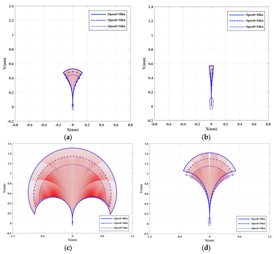
Figure 2. The finite-time reachable sets of “MARINER” and “TANKER”. (a) ${\overline{RS}}_{F1}$ of “MARINER” for the case t_r = 2 min; (b) ${\overline{RS}}_{F1}$ of “TANKER” for the case t_r = 2 min; (c) ${\overline{RS}}_{F1}$ of “MARINER” for the case t_r = 5 min; (d) ${\overline{RS}}_{F1}$ of “TANKER” for the case t_r = 5 min.

Apparently, Equation (15) is compatible with Equation (2), so we can treat the finite-time reachable sets ${\overline{RS}}_{F1}$ as the ship domain. Similar to the ship’s domains, the ship’s finite-time reachable set can be utilized to determine the collision risk between ships.

The ship’s finite-time reachable set essentially predicts its potential range of motion within a given period based on the ship’s dynamic model, similar to the approach employed in MPC for collision avoidance. For instance, ref. [40] demonstrated the feasible trajectories for prospective N_p steps of ship motion, which were computed using a discrete dynamical model of the vessel. Compared to the trajectories illustrated in Figure 2, the feasible paths presented in [40] were predicated on the assumption that rudder angle variations occurred at each computational step. Considering Rule 8 of COLREGs, small alterations of course should be avoided. Thus, when the trajectory calculation period is relatively short, it is advisable to maintain a constant rudder angle. Naturally, this is also contingent upon the vessel’s inherent maneuvering characteristics—as evidenced by Figure 2a,b, where distinct trajectory variations emerge over 2 min computation periods for different vessels. Hence, this study underscores the imperative of thoroughly considering the vessel’s maneuverability in practical applications, selecting an appropriate reaction time as the computation period to ensure compliance with the requirements of COLREGs.

As indicated in [14], uncertainties from external environmental changes, variations in the vessel itself, and sensor noise will result in uncertainties in the navigational trajectories derived from the motion model. Consequently, in practical applications, the reachable set for the vessel can yield accurate results only under conditions where the vessel model is sufficiently precise. Moreover, Equation (13) provides the full operation range of the actuators without consideration with the constrains caused by the meeting rules, such as Rule 13–17. If we consider the particular encounter situation, the operating range of the actuators will be further reduced, resulting in a corresponding contraction of the trajectory range obtained. If the complete operational range of the actuators is considered, it will only broaden the spatial range during subsequent risk assessments.

In order to obtain the ship’s finite-time reachable set, we must resolve a substantial number of vessel motion trajectories, which demands considerable computational resources. Fortunately, modern parallel computing technologies utilizing GPUs facilitate the efficient solution of differential equations, enabling computations of the limited time reach set to be completed within seconds, thereby satisfying the requirements of practical engineering applications.

4. Risk Assessment Base on Ship’s Finite-Time Reachable Set

The ship’s finite-time reachable set ${\overline{RS}}_{FK}$ reflects some features of the ship and cover its operations, so it can be considered as a criterion to distinguish safe areas and those areas where a collision may arise.

The risk assessment based on ship’s reachable sets fundamentally relies on the principle that a collision between vessels cannot occur if they do not come into contact within a spatial context. The ship’s finite-time reachable set defines the spatial area that the ship can access within a specified time. If there are no other vessels or obstacles present within this area, it indicates that the region where OS may pass through during that time is free of other targets, thus clearly indicating that the navigational risk for OS is zero. Conversely, if OS also lies outside the reachable set of other vessels, it will not obstruct their navigation within a given time and, consequently, will not pose a threat to them. Therefore, we can obtain the following property of ship’s finite-time reachable set.

Property 1.

$R_{o,k}=0, \mathrm{if}\hspace{0.33em}{P}_t^k\notin {\overline{RS}}_{Fk}(t_r,x_s)$

Property 1 means that if ship’s finite-time reachable set contains no other vessels or navigational hazards, then the subject vessel presents no collision risk. The ship’s finite-time reachable set can be considered as a new ship domain model if we qualitatively define the risk value when a TS enters the reachable set ${\overline{RS}}_{FK}$, that is

$$R_{o,k}=F_R(X)=F_R(P_t^k)=\left\{\begin{array}{l}1,\hspace{1em}{P}_t^k\in {\overline{RS}}_{Fk}(t_r,x_s)\\ 0,\hspace{1em}{P}_t^k\notin {\overline{RS}}_{Fk}(t_r,x_s)\end{array}\right.$$

(16)

Additionally, as the computation of the reachable set encompasses the states of the vessel at all positions within it, it facilitates a quantitative assessment of the potential consequences of a collision occurring within that set.

According to Property 1, a collision between vessels can only occur under the condition that their ship’s finite-time reachable sets intersect. Moreover, the greater the overlap between two vessels’ finite-time reachable sets, the more potential locations for collisions arise, thereby increasing the probability of such incidents. Specifically, the ratio of the overlapping region’s area to the area of the vessel’s finite-time reachable set can serve as a quantitative representation of the collision probability for a particular vessel.

Thus, the intersection area between the two ships’ finite-time reachable sets is used to measure the possibility of the potential collision. Define the intersection area by

$$I={\overline{RS}}_{Fk}^O\cap {\overline{RS}}_{Fk}^T$$

(17)

where ${\overline{RS}}_{Fk}^O$ and ${\overline{RS}}_{Fk}^T$ are ship’s finite-time reachable sets of OS and TS, respectively.

Therefore, the probability of collision between two ships can be described through geometric probability [29]. The collision probability of own ship can be given by the following equation

$$P_o={\displaystyle \frac{S(I)}{S({\overline{RS}}_{Fk}^O)}}$$

(18)

where $S(\cdot )$ denotes the geometric area of the set. We can also obtain the collision probability of TS

$$P_T={\displaystyle \frac{S(I)}{S({\overline{RS}}_{Fk}^T)}}$$

(19)

Equations (18) and (19) consistently align with the previously articulated understanding of the ship’s finite-time reachable set. If the intersection I is empty, i.e., $S(I)=0$, the probability of OS is 0. If I is not empty, the collision probability is related to the size of the intersection area and the vessel’s finite-time reachable set. Typically, the size of $\overline{RS}$ is directly proportional to the vessel’s speed and the reserved action time. The size of the intersection area depends on the situation between own ship and target ship. Thus, P_o and P_t are time-varying, influenced by factors affecting I and $\overline{RS}$, such as the ship speed, the reserved action time of the navigator and their respective situations.

According the definition of Equations (18) and (19), we can obtain the following property.

Property 2.

Both $P_{\mathrm{O}}$ and $P_T$ are continuous.

Property 2 can be easily proved, since the ship’s motion is always continuous whether $I=\varnothing$ or not.

Compared to the other collision probability models, Equations (18) and (19) is a comprehensive collision probability framework which considers vessel maneuverability characteristics, environmental conditions, and navigators’ experiential factors of both vessels. This correlation exists because collision probability is strongly associated with the ship’s finite-time reachable sets, which are themselves intrinsically linked to vessel maneuverability characteristics, prevailing environmental conditions, and the reaction time of navigators during maneuvering operations. It is also COLREGs-compatible and continuous according to the definition of the ship’s finite-time reachable set.

The negative consequences from a ship collision accident are not only related to both sides of the accident but also social costs, repair costs, costs of salvage, rescue, and other mitigation measures after the collision happens. According to [46], the final costs depend on the ship collision damage, which is proportional to the impact force [47,48]. In other words, there exists a cost function with respect to the total exerted force $F_n$, i.e.,

$$C_{OT}=C(F_n)$$

(20)

Strictly speaking, the cost function $C(\cdot )$ is a nonlinear function with a complicated form. For the convenience of the practical implementation, we only consider the strength of the force; then, the loss $C_{OT}$ of OS can be approximated by its linearization at $F$, that is

$$C_{OT}=b_{OT}\left|F\right|$$

(21)

where $\left|F\right|$ denotes the strength of the impact force, and it can be estimated according to impulse-momentum theorem; $b_{OT}$ is the coefficient of the linearization form.

Although a collision inevitably occurs within the intersection area of the finite-time reachable sets of two vessels, the intersection area comprises intersection points of these vessel trajectories, meaning that every point within this area could potentially be a collision location. Figure 3 illustrates the intersections of the vessel trajectories in this area. Therefore, it is necessary to calculate the collision losses at all possible points to determine the range of potential collision losses. Fortunately, the ship’s finite-time reachable sets of the vessels are derived from the vessels’ trajectories, and the states of the vessels at every intersection point can be obtained through the vessel dynamics model, which can be utilized to calculate collision losses. The method for calculating collision losses at each intersection point is outlined as follows.

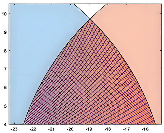
Figure 3. Ship trajectories in the intersection area.

For any point in the intersection area, the navigational velocities of both vessels can be derived from their dynamic models. Let vectors, ${\overrightarrow{v}}_o$ and ${\overrightarrow{v}}_t$, represent the velocities of OS and TS before collision, respectively. It is assumed that the two vessels collide at their navigational velocities, ${\overrightarrow{v}}_o$ and ${\overrightarrow{v}}_t$, and at the moment of impact, both vessels achieve identical velocities, leading to the maximum loss of kinetic energy and resulting in the worst consequences.

According to the principle of conservation of momentum, the post-collision velocity $\overrightarrow{v}$ can be described by the following equation.

$$\overrightarrow{v}={\displaystyle \frac{m_o{\overrightarrow{v}}_o+m_t{\overrightarrow{v}}_t}{m_o+m_t}}$$

(22)

where $m_o$ and $m_t$ denote the mass of OS and TS, respectively, ${\overrightarrow{v}}_o$ and ${\overrightarrow{v}}_t$ denote the speed of OS and TS before collision, respectively. Then, the post-collision outcomes can be calculated according to the momentum theorem as follows

$$\left\{\begin{array}{l}{F}_o={\displaystyle \frac{1}{t_{\delta }}}(m_o{\overrightarrow{v}}_o-m_o\overrightarrow{v})\\ F_t={\displaystyle \frac{1}{t_{\delta }}}(m_t{\overrightarrow{v}}_t-m_t\overrightarrow{v})\end{array}\right.$$

(23)

where $F_o$ and $F_t$ denote the compact force of OS and TS, respectively, $t_{\delta }$ is the time interval of the collision. Thus, we can obtain the strength of the impact force as follows

$$\left\{\begin{array}{l}|F_o|={\displaystyle \frac{1}{t_{\delta }}}|m_o{\overrightarrow{v}}_o-m_o\overrightarrow{v}|\\ |F_t|={\displaystyle \frac{1}{t_{\delta }}}|m_t{\overrightarrow{v}}_t-m_t\overrightarrow{v}|\end{array}\right.$$

(24)

where $|·|$ denotes the modulo operation. From Equation (23), we can obtain the loss for every point in the intersection area, that is

$$\left\{\begin{array}{l}{C}_{OT}=b_{OT}\left|F_o\right|\\ C_{TO}=b_{TO}\left|F_t\right|\end{array}\right.$$

(25)

where $C_{TO}$ denote the loss of TS at a specific point, while $b_{TO}$ is the corresponding coefficient. For the whole intersection area, we can obtain the maximum and minimum losses of both vessels, i.e.,

$$\left\{\begin{array}{l}{C}_{O\max }=\max \left\{C_{OT},P_t^k\in I\right\}\\ C_{O\min }=\min \left\{C_{OT},P_t^k\in I\right\}\\ C_{T\max }=\max \left\{C_{TO},P_t^k\in I\right\}\\ C_{T\min }=\min \left\{C_{TO},P_t^k\in I\right\}\end{array}\right.$$

(26)

According [40,41], the collision probability and the consequence need to be considered together for risk assessment. The risk can be assessed as

$$R=P\cdot C$$

(27)

where P denotes the collision probability and C denotes the consequence of the collision.

From (25), we can assess the boundary of the potential collision risk. For OS, it can be expressed as

$$R_{o\max }=P_o\cdot C_{o\max }\hspace{0.33em}\mathrm{and}\hspace{0.33em}{R}_{o\min }=P_o\cdot C_{o\min }\hspace{0.33em}$$

(28)

and for TS, it can be expressed as

$$R_{T\max }=P_T\cdot C_{T\max }\hspace{0.33em}\mathrm{and}\hspace{0.33em}{R}_{T\min }=P_T\cdot C_{T\min }\hspace{0.33em}$$

(29)

It is remarkable that the collision risks obtained using the above methods are all continuous with respect to time. Property 2 already shows the continuity of the probability. We only need to prove the continuity of the loss. It is obvious that Equations (28) and (29) are continuous. Moreover, the intersection area is also connected and dense. Therefore, the extreme points of the loss function are also continuous. It means that the requirements R₂ and R₂ are both satisfied.

For engineering practice, the states of OS are provided by its navigation devices, while the states of TS can also be obtained from the AIS device equipped on own ship. Usually, AIS information includes the position, speed, and yaw angle of the target ship, as well as its length and width. However, AIS transmission delays and inherent sensor noise may introduce inaccuracies in the data pertaining to target vessels. It is imperative to implement filtering algorithms to obtain more precise vessel state information in order to ensure the reliability of collision risk assessments. Thus, the risk assessment algorithm can be written as follows.

Algorithm 1 provides a risk assessment process for ships with collision risks, which can be conducted in real time during ship navigation. Furthermore, this algorithm not only quantifies the collision risk but also establishes the upper and lower boundaries of the risk.

Algorithm 1. Collision Risk Assessment Algorithm

► Given: $X_o$: the state vector of own ship      $X_T$: the state vector of target ships     ${\overline{RS}}_o$: get own ship’s finite-time reachable set, from own ship state vector     ${\overline{RS}}_T$: get target ship’s finite-time reachable set, from target ship state vector    $S({\overline{RS}}_o)$: get the area of own ship’s reachable set, from the reachable set boundary of own ship    $S({\overline{RS}}_T)$: get the area of target ship’s reachable set, from the reachable set boundary of target ship   $I_{{\overline{RS}}_o\cap {\overline{RS}}_T}$: get the intersection boundary area of the reachable set  $S(I_{{\overline{RS}}_o\cap {\overline{RS}}_T})$: get the area of target ship’s reachable set, from the reachable set boundary of target ship ► Initialize: $b_{OT}$, $b_{TO}$, $t_{\delta }$, $U_O$, $U_T$, $T_r$ if $I_{{\overline{RS}}_o\cap {\overline{RS}}_T}=0$   $P_o={\displaystyle \frac{S(I_{{\overline{RS}}_o\cap {\overline{RS}}_T})}{S({\overline{RS}}_o)}}=0$   $P_T={\displaystyle \frac{S(I_{{\overline{RS}}_o\cap {\overline{RS}}_T})}{S({\overline{RS}}_T)}}=0$   $R_o=R_T=0$  else   $P_{o,k}={\displaystyle \frac{S(I_{{\overline{RS}}_o\cap {\overline{RS}}_T})}{S({\overline{RS}}_o)}}$   $P_t^k={\displaystyle \frac{S(I_{{\overline{RS}}_o\cap {\overline{RS}}_T})}{S({\overline{RS}}_T)}}$   $C_{OT}={\displaystyle \frac{b_{OT}}{t_{\delta }}}|m_o{\overrightarrow{v}}_o-m_o\overrightarrow{v}|$   $C_{TO}={\displaystyle \frac{b_{TO}}{t_{\delta }}}|m_t{\overrightarrow{v}}_t-m_t\overrightarrow{v}|$   $\left\{\begin{array}{l}{C}_{O\max }=\max \left\{C_{OT},P_t^k\in I\right\}\\ C_{O\min }=\min \left\{C_{OT},P_t^k\in I\right\}\\ C_{T\max }=\max \left\{C_{TO},P_t^k\in I\right\}\\ C_{T\min }=\min \left\{C_{TO},P_t^k\in I\right\}\end{array}\right.$   $R_{o\max }=P_o\cdot C_{o\max }\mathrm{and}{R}_{o\min }=P_o\cdot C_{o\min }$   $R_{T\max }=P_T\cdot C_{T\max }\mathrm{and}{R}_{T\min }=P_T\cdot C_{T\min }$ end

5. Simulation Studies

To validate the proposed collision risk assessment method, this paper conducted simulation experiments involving the vessels “TANKER” and “MARINER”, exploring three encounter situations: head-on, crossing, and overtaking. These three encounter situations represent the most common situations faced by vessels during collision avoidance maneuvers. The algorithm was implemented and executed using MATLAB 2024a. The simulation experiments were conducted on a system with an AMD Ryzen9 7940HS processor running at 4.00 GHz and 32.0 GB of RAM.

In order to more clearly delineate the distinctive characteristics of the method presented in this paper, we simultaneously provide the risk assessment results based on both the DCPA method and the APF method. The APF method is formulated based on the following equation [27,28,31]:

$$\begin{array}{cc}\hfill R_{o,k}(p_o,p_k)=& U_{att}(p_o,p_k)+U_{rep}(p_o,p_k)\hfill \\ \hfill =& \left\{\begin{array}{l}{\displaystyle \frac{1}{2}}{k}_{att}{\rho }^2(p_o,p_g)+{\displaystyle \frac{1}{2}}{k}_{rep}{\left({\displaystyle \frac{1}{\rho \left(p_o,p_k\right)}}-{\displaystyle \frac{1}{{\rho }_0}}\right)}^2\hspace{0.33em}\hspace{0.33em},0\le \rho \left(p_o,p_k\right)\le {\rho }_0\\ {\displaystyle \frac{1}{2}}{k}_{att}{\rho }^2(p_o,p_g)\hspace{1em}\hspace{1em}\hspace{1em}\hspace{1em}\hspace{1em}\hspace{1em}\hspace{1em}\hspace{1em}\hspace{1em}\hspace{1em}\hspace{1em},\rho \left(p_o,p_k\right)>{\rho }_0\end{array}\right.\hfill \end{array}$$

(30)

where p_o and p_k represent the positions of the OS and TS, respectively; U_att and U_rep denote the attractive potential field and the repulsive potential field, respectively; k_att and k_rep are the coefficients of the attractive potential field and the repulsive potential field, respectively; ρ(p_o, p_g) denotes the distance between the own ship and the goal point, ρ(p_o, p_k) denotes the distance between the OS and TS; and ρ₀ is the influence radius of the TS. The parameters specified in [27] are implemented in the simulations, i.e., k_att = 5, k_rep = 200, and ρ₀ = 2.

The flow diagram of simulation experiments involving the vessels “TANKER” and “MARINER” is shown in Figure 4. The simulations start with the initialization of the motion models of the vessels and end with the final simulation time t_f. In our studies, t_f = 2500s. For every loop, the simulation program will update the positions of the vessels according to their motion models and their finite-time reachable sets. Then, the program will determine whether two finite-time reachable sets have intersection. If there is no intersection, the program returns to the decision of whether to terminate; otherwise, it proceeds to further calculate the collision probability and risk. Then, the simulation program will perform the calculation for the next step. The simulation period is one second so that the time is updated with t = t + 1. After spending 2500 steps, we can obtain a set of curves representing the navigational situation.

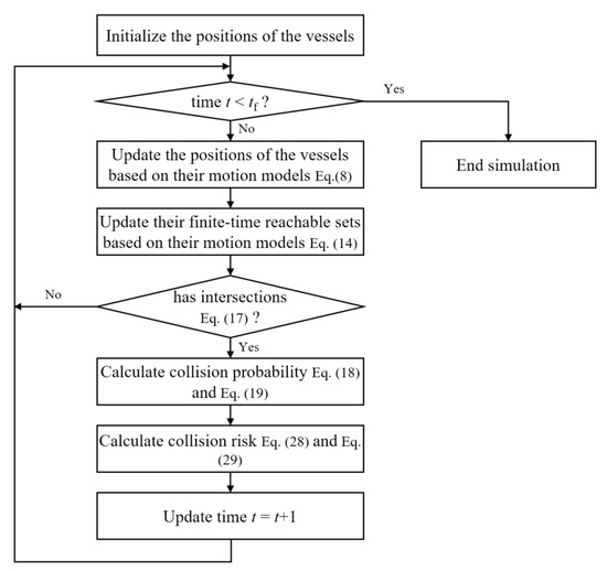
Figure 4. Flow diagram of simulation experiments involving the vessels “TANKER” and “MARINER”.

The initial conditions in head-on encounter situation are provided in Table 2. The collision risk prediction between “TANKER” and MARINER during encounter situations is illustrated in Figure 5. In Figure 5a, the red and blue regions represent the finite-time reachable sets of “TANKER” and “MARINER”, respectively, showcasing their respective navigation trajectories. The pink and green three-dimensional curves depict the collision probabilities of “TANKER” and “MARINER” as they evolve over time. Figure 5b shows how the collision probability varies over time during the encounter between “TANKER” and “MARINER”. As time progresses, the distance between the two vessels decreases while the intersection area of their reachable sets increases, followed by a phase in which the vessels begin to distance themselves again. Consequently, the probability of collision initially rises and subsequently diminishes.

Table 2. Initial conditions in head-on situation.

Ship	Position (nm)	Velocity (knots)	Course (°)
TANKER(OS)	(0, 7)	18	0
MARINER(TS)	(2, 32)	14	190

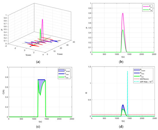
Figure 5. Simulation results of the head-on encounter situation of “TANKER” and “MARINER”, (a) the navigation trajectories of “TANKER” and “MARINER”, along with the three-dimensional curves depicting the variation in collision probabilities over time; (b) the collision probability curves for “TANKER” and “MARINER”; (c) the range of collision consequences; (d) the maximum and minimum collision risks for “TANKER” and “MARINER” compared with the risk estimated by DCPA (dotted-line) and APF (dash-dotted-line) methods.

In Figure 5c, the blue and green curves record the maximum and minimum consequences of a collision between “TANKER” and “MARINER” over continuous time intervals. The blue area indicates the range of collision consequences at various moments in time. As the vessels navigate, the intersection area of their reachable sets changes, thereby causing the consequences of a collision to evolve continuously. The magnitude of the collision consequences is influenced not only by the vessels’ speeds and masses but also by their positions and velocity directions. The position and velocity direction that yield the maximum consequence remains constant, while that yielding the minimum consequence changes over time. As a result, when the collision consequences are non-zero, the maximum value remains stable, whereas the minimum value first decreases and then increases over time.

Figure 5d illustrates the maximum and minimum collision risks for “TANKER” and “MARINER”, showing how these values change with time. The blue and green curves correspond to the maximum and minimum collision risks, respectively. The trend observed indicates that the collision risks first increase and then decrease, allowing us to ascertain that the blue region represents the variation range of collision risk for the “TANKER” and “MARINER” during their navigation. The dotted line in Figure 5d shows DCPA value between “TANKER” and “MARINER”. For this encounter situation, DCPA is a small constant. The dashed–dotted line in Figure 5d illustrates the risk estimated by APF method. Obviously, the risk estimated by APF method is relatively larger than the results of other methods.

The initial conditions in crossing encounter situation are given in Table 3. Figure 6a illustrates the navigation trajectories of “TANKER” and “MARINER”, along with the three-dimensional curves depicting the variation in collision probabilities over time. Figure 6b presents the collision probability curves for “TANKER” and “MARINER”, represented by the pink and green lines, respectively. Figure 6c indicates the range of collision consequences throughout this continuous process. Figure 6d provides a comprehensive overview of the collision risk experienced by “TANKER” and “MARINER” during their entire operation, from which specific moments of maximum collision consequences can be clearly identified, along with the collision risks at different times. It can be concluded that the collision risk at any given moment is consistently confined between the determined maximum and minimum values for that time. Similar to Figure 5, the dotted line and dash–dotted line demonstrate the DCPA and the risk estimated by the APF method between two vessels. Compared to the head-on encounter situation, the DCPA increases. Nevertheless, the risk estimated by both the proposed methodology and the APF method demonstrate a commensurate decrease, which confirms with the observed variation in DCPA.

Table 3. Initial conditions in crossing situation.

Ship	Position (nm)	Velocity (knots)	Course (°)
TANKER(OS)	(0, 0)	18	0
MARINER(TS)	(12, 13)	14	280

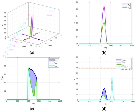
Figure 6. Simulation results of the crossing encounter situation of “TANKER” and “MARINER”, (a) the navigation trajectories of “TANKER” and “MARINER”, along with the three-dimensional curves depicting the variation in collision probabilities over time; (b) the collision probability curves for “TANKER” and “MARINER”; (c) the range of collision consequences; (d) the maximum and minimum collision risks for “TANKER” and “MARINER” compared with the risk estimated by DCPA (dotted line) and APF (dash–dotted line) methods.

Table 4 provides the initial conditions of an overtaking encounter situation. Figure 7 depicts the collision risk during the overtaking process between “TANKER” and “MARINER”. Figure 7a illustrates the navigation trajectories of both vessels during overtaking, along with the curves representing the variation in collision probabilities for “TANKER” and “MARINER” throughout this process. From Figure 7b, the values of collision probabilities at different time points can be clearly observed, with the pink curve representing the collision probability of “TANKER” and the green curve representing that of “MARINER”. The continuous changes in the intersection area of their reachable sets lead to a dynamic alteration in collision probability over time.

Table 4. Initial conditions in overtaking situation.

Ship	Position (nm)	Velocity (knots)	Course (°)
TANKER(OS)	(0, 7)	18	0
MARINER(TS)	(3, 9)	14	345

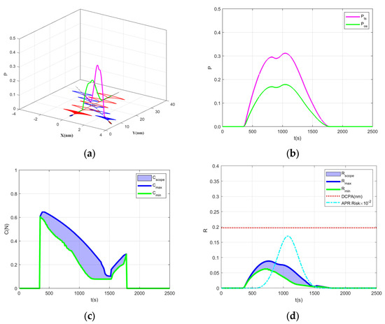
Figure 7. Simulation results of the overtaking encounter situation of “TANKER” and “MARINER”: (a) the navigation trajectories of “TANKER” and “MARINER”, along with the three-dimensional curves depicting the variation in collision probabilities over time; (b) the collision probability curves for “TANKER” and “MARINER”; (c) the range of collision consequences; (d) the maximum and minimum collision risks for “TANKER” and “MARINER” compared with the risk estimated by DCPA (dotted line) and APF (dashed–dotted line) methods.

Figure 7c describes the trend of collision consequences for “TANKER” and “MARINER” during the overtaking maneuver. The collision consequences initially decrease gradually due to the influence of varying positions and velocity directions within the intersection area of their reachable sets, followed by a gradual increase after some time. The blue and green curves denote the maximum and minimum values of the collision consequences, respectively, while the area between these extremes represents the range of collision consequences throughout the entire process. Figure 7d presents the collision risk for “TANKER” and “MARINER” under the assumptions of collision probability and consequences, elevating the one-dimensional concept of risk into a two-dimensional space, thereby illustrating the range of collision risk values. The dotted line in Figure 7d also demonstrates a larger DCPA value between two vessels than the head-on case, but smaller than the crossing case. The risk estimated by APF method is illustrated by the dashed–dotted line in Figure 7d and is also much smaller than the crossing case.

In the above simulation, the speeds of “TANKER” and “MARINER” remains constant throughout the specific simulation. The variance in collision risk is closely associated with the vessels’ courses. It is observed that the highest risk manifests during vessels head-on encountering, as this scenario yields the greatest probability and consequences of collision. From the perspective of the duration time, the high-risk situation in the head-on case persists for the shortest period when compared to the other two scenarios, while the longest duration of risk is observed in the overtaking encounter case. This observation aligns with the relative velocities of the simulation cases.

Moreover, all DCPA values between the two vessels remain constant. In the head-on scenario, DCPA is very small, thereby constituting a high-risk encounter situation. It conforms with the risk evaluation given by the proposed method. For the other two cases, the DCPA values are not compatible with the risk assessment results. This discrepancy may be attributable to the explicit consideration of consequence within the proposed risk assessment framework. Compared to DCPA method, the risk evaluated by the proposed algorithm varies according to the situational dynamics between the own vessel and target vessel. The trend of risk variation is critically important for navigators in formulating collision avoidance decisions, as all collision avoidance maneuvers are designed to achieve risk reduction. Therefore, if the evaluated risk exhibits an upward trend, the navigator must maintain heightened vigilance and stand prepared to execute collision avoidance procedures.

In comparison to the APF method, the approach proposed in this paper exhibits a consistent variation in the assessed risk values. However, it demonstrates superior capability in collision risks at an earlier stage. This advantage may be attributed to the fact that the risks indicated by the APF method are primarily generated by repulsive forces, whose effective range is confined to within 2 nm in the simulations.

The results of the above simulations also indicate that, due to the continuous nature of collision probabilities and consequences, which can fluctuate based on the vessels’ positions and respective states, we can conclude that the collision risk always remains continuous. It effectively captures the collision risk throughout the entire navigation process of the vessels, enabling a quantitative prediction of the collision risk range. Furthermore, the shape of the probability curve closely resembles that of the collision risk curve, which is particularly evident in their shared patterns of variation. It implies that the probability of risk serves as the determining factor in these simulation scenarios. Consequently, in most cases, the probability of risk can be employed as a reliable representation of collision risk.

Certainly, the aforementioned simulations only consider three typical encounter scenarios between two vessels and do not account for situations involving multiple vessels. In fact, when addressing the complexities of multi-vessel encounters, it is generally feasible to categorize these scenarios into pairwise encounters for individual risk evaluation, followed by a comprehensive assessment of navigational risks.

6. Conclusions

This study examined ship collision risk based on the attributes in their reachability. The ship’s finite-time reachable set is introduced to set up the connection between collision risk, the vessel’s dynamics, its current states, and the permissible actions of the navigator. A new quantitative collision risk assessment algorithm is developed based on the ship’s finite-time reachable set so that it can take advantage of the dynamic models of vessels and integrates factors such as the vessel’s current states, environmental conditions, and navigator characteristics. The probability of collision is characterized by the intersection of the finite-time reachable sets of the involved vessels. Moreover, the algorithm is continuous and only depends on the current states and parameters of OS and TS. It can dynamically provide both upper and lower bounds of collision risk, thereby equipping the navigator with enhanced information for informed collision avoidance decisions.

Issues such as uncertainties and constrained waterways are also major concerns in the field of maritime navigation safety. Although this paper does not delve into these matters in detail, the proposed methodology offers a potential approach to address these challenges. Furthermore, while the proposed collision risk assessment algorithm based on the finite-time reachable set still regards the navigator as the primary operator in vessel navigation, taking into account their “action time”, it can also be adapted for risk assessment in unmanned vessels by treating the response time of intelligent navigation systems as a similar parameter.

It is noteworthy that the proposed method based on the ship’s reachable set, which contains all possible trajectories within a specified time, not only provides collision risk assessment results but can also be employed to select feasible trajectories for collision avoidance during decision-making. If there exist trajectories that circumvent the intersection area between two ship’s finite-time reachable set, these trajectories can be candidates for the navigator as making the collision avoidance decision and the operations of propeller and rudder are also provided.

References

- Antão, P.; Sun, S.; Teixeira, A.P.; Guedes Soares, C. Quantitative assessment of ship collision risk influencing factors from worldwide accident and fleet data. Reliab. Eng. Syst. Saf. 2023, 234, 109166. [Google Scholar] [CrossRef]
- Osborne, M.; Magee, Z.; Deliso, M. Container Ship Collides with Anchored US-Flagged Oil Tanker in North Sea. Available online: https://abcnews.go.com/International/us-flagged-oil-tanker-collides-container-ship-north/story?id=119630008 (accessed on 11 March 2025).
- Dominguez-Péry, C.; Vuddaraju, L.N.R.; Corbett-Etchevers, I.; Tassabehji, R. Reducing maritime accidents in ships by tackling human error: A bibliometric review and research agenda. J. Shipp. Trd. 2021, 20, 6. [Google Scholar] [CrossRef]
- Zhang, X.; Wang, C.; Jiang, L.; An, L.; Yang, R. Collision-avoidance navigation systems for maritime autonomous surface ships: A state of the art survey. Ocean Eng. 2021, 235, 109380. [Google Scholar] [CrossRef]
- Aylward, K.; Weber, R.; Lundh, M.; MacKinnon, S.N.; Dahlman, J. Navigators’ views of a collision avoidance decision support system for maritime navigation. J. Navig. 2022, 75, 1035–1048. [Google Scholar] [CrossRef]
- Fujii, Y.; Tanaka, K. Traffic Capacity. J. Navig. 1971, 24, 543–552. [Google Scholar] [CrossRef]
- Wang, N.; Meng, X.; Xu, Q.; Wang, Z. A unified analytical framework for ship domains. J. Navig. 2009, 62, 643–655. [Google Scholar] [CrossRef]
- Szlapczynski, R.; Szlapczynska, J. Review of ship safety domains: Models and applications. Ocean Eng. 2017, 145, 277–289. [Google Scholar] [CrossRef]
- Li, W.; Cheng, K.; Shi, G.; Desrosiers, R.; Wang, X. Ship domain models: Reviewing the advancements and exploring the future directions in the maritime autonomous surface ships. Ocean Eng. 2025, 326, 120935. [Google Scholar] [CrossRef]
- Zheng, K.; Jiang, Y.; Zhou, S.; Xue, Y. A comprehensive spatiotemporal metric for ship collision risk assessment. Ocean Eng. 2022, 256, 112446. [Google Scholar] [CrossRef]
- Zheng, K.; Chen, Y.; Jiang, Y.; Qiao, S. A SVM based ship collision risk assessment algorithm. Ocean Eng. 2020, 202, 107062. [Google Scholar] [CrossRef]
- Kang, L.; Lu, Z.; Meng, Q.; Gao, S.; Wang, F. Maritime simulator based determination of minimum DCPA and TCPA in head-on ship-to-ship collision avoidance in confined waters. Transp. A Transp. Sci. 2019, 15, 1124–1144. [Google Scholar] [CrossRef]
- Ha, J.; Roh, M.-I.; Lee, H.-W. Quantitative calculation method of the collision risk for collision avoidance in ship navigation using the CPA and ship domain. J. Comput. Des. Eng. 2021, 8, 894–909. [Google Scholar] [CrossRef]
- Yuan, X.; Zhang, D.; Zhang, J.; Zhang, M.; Guedes Soares, C. A novel real-time collision risk awareness method based on velocity obstacle considering uncertainties in ship dynamics. Ocean Eng. 2021, 220, 108436. [Google Scholar] [CrossRef]
- Liu, Z.; Zhang, B.; Zhang, M.; Wang, H.; Fu, X. A quantitative method for the analysis of ship collision risk using AIS data. Ocean Eng. 2023, 272, 113906. [Google Scholar] [CrossRef]
- Chen, Y.; Liu, Z.; Zhang, M.; Yu, H.; Fu, X.; Xiao, Z. Dynamics collision risk evaluation and early alert in busy waters: A spatial-temporal coupling approach. Ocean Eng. 2024, 300, 117315. [Google Scholar] [CrossRef]
- Cheng, K.; Li, W.; Zhou, Y.; Shi, G.; Wang, X. A novel fuzzy comprehensive evaluation method for ship collision risk. Ocean Eng. 2025, 332, 121462. [Google Scholar] [CrossRef]
- Korupoju, A.K.; Kapadia, V.; Vilwathilakam, A.S.; Samanta, A. Ship collision risk evaluation using AIS and weather data through fuzzy logic and deep learning. Ocean Eng. 2025, 318, 120116. [Google Scholar] [CrossRef]
- Lin, C.; Zhen, R.; Tong, Y.; Yang, S.; Chen, S. Regional ship collision risk prediction: An approach based on encoder-decoder LSTM neural network model. Ocean Eng. 2024, 296, 117019. [Google Scholar] [CrossRef]
- Shi, J.; Liu, Z.; Feng, Y.; Wang, X.; Zhu, H.; Yang, Z.; Wang, J.; Wang, H. Evolutionary model and risk analysis of ship collision accidents based on complex networks and DEMATEL. Ocean Eng. 2024, 305, 117965. [Google Scholar] [CrossRef]
- Liu, J.; Zhang, J.; Yang, Z.; Zhang, M.; Tian, W. A game-based decision-making method for multi-ship collaborative collision avoidance reflecting risk attitudes in open waters. Ocean. Coast. Manag. 2024, 259, 107450. [Google Scholar] [CrossRef]
- Li, P.; Wang, Y.; Yang, Z. Risk assessment of maritime autonomous surface ships collisions using an FTA-FBN model. Ocean Eng. 2024, 309, 118444. [Google Scholar] [CrossRef]
- Wang, J.; Wu, J.; Li, Y. The driving safety field based on driver–vehicle–road interactions. IEEE Trans. Intell. Transp. Syst. 2015, 16, 2203–2214. [Google Scholar] [CrossRef]
- Wang, J.; Wu, J.; Zheng, X.; Ni, D.; Li, K. Driving safety field theory modeling and its application in pre-collision warning system. Transp. Res. Part C Emerg. Technol. 2016, 72, 306–324. [Google Scholar] [CrossRef]
- Zuo, D.; Bian, Z.; Zuo, F.; Ozbay, K. Composite safety potential field for highway driving risk assessment. Accid. Anal. Prev. 2025, 220, 108080. [Google Scholar] [CrossRef]
- Lei, C.; Zhao, C.; Chen, K.; Ji, Y.; Du, Y. A novel ellipsoidal safety potential field model for quantifying driving risk. Transp. A Transp. Sci. 2025, 6, 1–30. [Google Scholar] [CrossRef]
- Li, H.; Wang, X.; Wu, T.; Ni, S. A COLREGs-compliant ship collision avoidance decision-making support scheme based on improved APF and NMPC. J. Mar. Sci. Eng. 2023, 11, 1408. [Google Scholar] [CrossRef]
- He, Z.; Chu, X.; Liu, C.; Wu, W. A novel model predictive artificial potential field based ship motion planning method considering COLREGs for complex encounter scenarios. ISA Trans. 2023, 134, 58–73. [Google Scholar] [CrossRef]
- Tang, C.; Xia, J.; Wang, W.; Shang, H.; Ji, W.; Bao, Q.; Yang, D. A dynamic window model prediction of artificial potential field method for improving the coincidence of actual and predicted trajectory of underactuated planing craft. Ocean Eng. 2024, 313, 119351. [Google Scholar] [CrossRef]
- Gan, L.; Yan, Z.; Zhang, L.; Liu, K.; Zheng, Y.; Zhou, C.; Shu, Y. Ship path planning based on safety potential field in inland rivers. Ocean Eng. 2022, 260, 111928. [Google Scholar] [CrossRef]
- Kim, J.-H.; Jo, H.-J.; Kim, S.-R.; Choi, S.-W.; Park, J.-Y.; Kim, N. Comparison of collision avoidance algorithms for unmanned surface vehicle through free-running test: Collision risk index, artificial potential field, and safety zone. J. Mar. Sci. Eng. 2024, 12, 2255. [Google Scholar] [CrossRef]
- Isidori, A. Nonlinear Control Systems, 3rd ed.; Springer: London, UK, 1995; pp. 53–69. [Google Scholar]
- Guéguen, H.; Lefebvre, M.A.; Nasri, O.; Zaytoon, J. Safety verification and reachability analysis for hybrid systems. In Proceedings of the 17th World Congress the International Federation of Automatic Control, Seoul, Republic of Korea, 6–11 July 2008; Volume 41, pp. 8949–8959. [Google Scholar]
- Zhou, C.; Li, Y.; Zheng, W.; Wu, P.; Dong, Z. Safety Envelope Determination for Impaired Aircraft During Landing Phase Based on Reachability Analysis. In Proceedings of the 2018 Asia-Pacific International Symposium on Aerospace Technology; Springer: Singapore, 2019. [Google Scholar]
- Zhou, C.; Li, Y.; Zheng, W.; Wu, P.; Dong, Z. Safety analysis for icing aircraft during landing phase based on reachability analysis. Math. Probl. Eng. 2018, 2018, 3728241. [Google Scholar] [CrossRef]
- Manzinger, S.; Pek, C.; Althoff, M. Using reachable sets for trajectory planning of automated vehicles. IEEE Trans. Intell. Veh. 2021, 6, 232–248. [Google Scholar] [CrossRef]
- Xiao, Y.; Xia, T.; Wang, H. Formal safety verification of non-deterministic systems based on probabilistic reachability computation. Syst. Control. Lett. 2025, 196, 106014. [Google Scholar] [CrossRef]
- Zhang, B.; Bai, Y.; Zhang, K.; Zheng, K.; Jiang, Y. Ship Dynamic Collision Avoidance Algorithm Based on Reachable Set. In Proceedings of the 37th Chinese Control and Decision Conference (CCDC 2025), Xiamen, China, 16–19 May 2025; pp. 5264–5269. [Google Scholar]
- Potočnik, P. Model predictive control for autonomous ship navigation with COLREG compliance and chart-based path planning. J. Mar. Sci. Eng. 2025, 13, 1246. [Google Scholar] [CrossRef]
- Huang, Y.; Chen, L.; Chen, P.; Negenborn, R.R.; van Gelder, P.H.A.J.M. Ship collision avoidance methods: State-of-the-art. Saf. Sci. 2020, 121, 451–473. [Google Scholar] [CrossRef]
- Terndrup Pedersen, P. Review and application of ship collision and grounding analysis procedures. Mar. Struct. 2010, 23, 241–262. [Google Scholar] [CrossRef]
- Wang, G.; Spencer, J.; Chen, Y. Assessment of a ship’s performance in accidents. Mar. Struct. 2002, 15, 313–333. [Google Scholar] [CrossRef]
- Fossen, T.I. Handbook of Marine Craft Hydrodynamics and Motion Control, 2nd ed.; Wiley: Hoboken, NJ, USA, 2021; pp. 135–180. [Google Scholar]
- Son, K.; Nomoto, K. On the coupled motion of steering and rolling of a high speed container ship. J. Soc. Nav. Archit. Jpn. 1981, 150, 232–244. [Google Scholar] [CrossRef]
- Fossen, T.I.; Perez, T. Marine Systems Simulator (MSS). Available online: https://github.com/cybergalactic/MSS (accessed on 1 June 2004).
- Kuznecovs, A.; Ringsberg, J.W.; Mallaya Ullal, A.; Janardhana Bangera, P.; Johnson, E. Consequence analyses of collision-damaged ships—Damage stability, structural adequacy and oil spills. Ships Offshore Struct. 2022, 18, 567–581. [Google Scholar] [CrossRef]
- Li, S.; Meng, Q.; Qu, X. An overview of maritime waterway quantitative risk assessment models. Risk Anal. 2012, 32, 496–512. [Google Scholar] [CrossRef]
- Brown, A.J.; Chen, D. Probabilistic method for predicting ship collision damage. Ocean. Eng. Int. J. 2002, 6, 54–65. [Google Scholar]
Disclaimer/Publisher’s Note: The statements, opinions and data contained in all publications are solely those of the individual author(s) and contributor(s) and not of MDPI and/or the editor(s). MDPI and/or the editor(s) disclaim responsibility for any injury to people or property resulting from any ideas, methods, instructions or products referred to in the content. |
© 2025 by the authors. Licensee MDPI, Basel, Switzerland. This article is an open access article distributed under the terms and conditions of the Creative Commons Attribution (CC BY) license (https://creativecommons.org/licenses/by/4.0/).