Abstract
For the ship pipe routing design (SPRD) problem, previous studies have mainly employed bio-inspired algorithms such as multi-objective ant colony optimization (MOACO), non-dominated sorting genetic algorithm II (NSGA-II), and multi-objective particle swarm optimization (MOPSO). This paper proposes a novel approach based on the multi-objective A* (MOA*) algorithm to solve the SPRD. First, the optimization objectives and constraints of the SPRD problem are defined, and then an MOA*-based routing framework is developed. The time and space complexities of the approach are analyzed, and key components such as the cost functions, the solution dominance relationship, dynamic probability-based pruning, and neighbor node exploration strategy are designed to enhance solution diversity and search efficiency. Additionally, a space cascade expansion method is proposed to improve the computational efficiency of the MOA* in large-scale grid spaces. Comparative studies with MOACO, NSGA-II, GA-A*, and gray wolf optimization (GWO) on simulated cases of varying complexities and practical piping scenarios demonstrate the effectiveness of the MOA*. Furthermore, the applicability of the MOA* is validated against practical piping requirements, including the rapid generation of sub-optimal solutions, non-orthogonal routing, and partitioned pipe layouts. Experimental results, supported by a C++/OpenGL-based prototype software, show that the MOA* requires no extensive parameter tuning, exhibits stable computational efficiency and optimization capability, and demonstrates competitive performance in Pareto-optimal diversity compared with other algorithms.
1. Introduction
Ship pipe route design (SPRD) is one of the crucial aspects of ship design engineering, directly impacting the safety, functionality, and economic efficiency of the vessel. The ship pipe system can be likened to the blood vessels of the human body, responsible for transporting various fluids such as fuel, lubricating oil, water, and air. A rational pipe layout not only effectively enhances the operational efficiency of the ship but also reduces maintenance costs and energy consumption. However, as modern ships trend towards larger sizes, greater complexity, and higher performance, SPRD faces significant challenges. For instance, it is necessary to arrange a large number of different types of pipes within limited space, avoiding interference between pipes and other ship structures, while also considering various requirements such as pipe length, bends number, space occupation, and installation costs. Moreover, SPRD accounts for approximately 50% of the entire detailed design workload of a ship, and other detailed design activities depend on it [1,2]. Although current CAD software, such as Catia, AVEVA Marine, CADDS 5, and FORAN, include pipe design modules and provide tools that can achieve a certain level of automated routing, there is still room for improvement in design efficiency and quality when dealing with complex ship structures and extensive piping tasks. Particularly in addressing multi-objective pipe route design, there are numerous shortcomings. Currently, pipe engineers primarily utilize these tools for interactive pipe route design. Therefore, how to achieve efficient automated design of ship pipe routes has become one of the pressing challenges.
To address these challenges, researchers have conducted extensive studies on the SPRD problem and proposed a variety of automated pipe routing algorithms. Generally, the existing algorithms can be classified from different perspectives. From the perspective of algorithm randomness, they can be divided into deterministic algorithms and probabilistic algorithms. From the perspective of pipe layout evaluation, they can be classified into single-objective optimization and multi-objective optimization (MOO). Due to the high complexity of SPRD, the requirements for algorithms vary across different scenarios. Developing a practical ship piping system typically requires the integration of multiple methods with distinct characteristics.
Research on SPRD based on deterministic algorithms primarily focuses on optimizing path length and bends objectives, with other objectives typically implemented as algorithm constraints. Classical methods include graph theory-based algorithms such as Dijkstra’s algorithm [3], A* algorithm [4], and Jump Point Search [5]. These algorithms aim to plan pipe routes through shortest-path searches. However, due to the inherently complex nature of SPRD, scholars aim to incorporate more objectives and constraints into automated pipe route design algorithms. As a result, many studies employ the weighted sum method, transforming multiple objectives into a single objective for optimization. This approach balances multiple objectives by setting weight coefficients for each objective. Especially for the research employing bio-inspired algorithms, such as genetic algorithms [6], ant colony optimization [7], gray wolf optimization [8], and hybrid algorithms [9]. Among these, some representatives are selected for further discussion. Fan et al. [7,10] proposed ship piping methods based on ant colony optimization and genetic algorithms, using weighted sums to integrate sub-objectives such as path length and bend count to achieve optimized pipe layouts. Dong et al. [11] utilized genetic algorithms, incorporating additional sub-objectives such as parallel routing and ease of installation into the weighted summation objective. Ha et al. [9] proposed combining the expert system’s evaluation scores with other objectives, such as path length and bend count, through weighted summation as the path’s objective. This approach offers the advantage of easily modifying pipe metrics through the expert system interface, making the system more practical.
With the development of SPRD, scholars have recognized that optimization methods converting multiple objectives into a single objective cannot comprehensively balance design goals and rely on the setting of weights. Therefore, in recent years, the application of multi-objective optimization to solve SPRD has gained attention. Multi-objective optimization can simultaneously balance conflicting objectives like pipe length, bend count, and location. Therefore, the evolutionary or swarm-based MOO algorithms, such as NSGA-II, MOACO, and MOPSO, are now mainstream approaches in this field. For instance, Niu et al. [12] proposed a SPRD method based on a multi-objective genetic algorithm, which can optimize three sub-objectives: path length, bends number, and overlapping length between branches, achieving optimized design of branched pipes. Dong et al. [13,14] and Yan et al. [15] used NSGA-II and MOACO to optimize complex ship pipe layouts, considering trade-offs among multiple objectives including path length, bends number, installation position, bending length limit, and pocket structure, and achieved good results by incorporating actual constraints. Lin and Zhang [16] proposed using MOPSO to optimize the pipe length, bends number, and parallel assembly length of multiple pipes, obtaining a Pareto optimal set of layout schemes. Jiang et al. [17], Yan et al. [18], and Zhang [19] proposed a collaborative layout optimization of ship pipes and connected equipment, offering a new direction to multi-objective optimization of ship pipes. In contrast to bio-inspired algorithms, deterministic search-based multi-objective algorithms such as the multi-objective A* (MOA*) have also been explored for path planning. For instance, Ren et al. [20] and Martins et al. [21] improved MOA*-based frameworks to enhance computational efficiency and solution accuracy in 2D environments. These methods can generate exact Pareto-optimal solutions and have shown promising results in multi-objective shortest path problems. However, applying MOA* to SPRD faces several challenges, such as high computational cost in large 3D grid spaces, the need to handle complex engineering constraints, and the relatively low diversity of Pareto-optimal solutions compared with bio-inspired algorithms. To the best of the authors’ knowledge, no existing studies have yet applied MOA*-based approaches to address the SPRD problem.
As artificial intelligence advances, reinforcement learning (RL) methods have also been attempted for path optimization and pipe route design. Wang et al. [22] utilized an improved Q-Learning algorithm to solve path planning problem in two-dimensional space, optimizing the path length and bends number, demonstrating the feasibility of RL in the field of pipe route design. Yang et al. [23] improved the parameter update and exploration strategy of the reinforcement learning actor-critic algorithm, showing good performance in ship trajectory planning. Kim et al. [24] integrated curriculum learning into reinforcement learning and applied it to address SPRD problem. Compared to A*, Jump Point Search, and other traditional reinforcement learning algorithms, the new algorithm reduces the time required for pipe routing and generates paths with fewer bends than those produced by A* and Jump Point Search. However, this method only focuses on two objectives, i.e., the pipe length and bends number, and incurs high computational costs during model training.
Based on the literature review above, we summarize and classify representative algorithms applicable to path planning and pipe routing design in Table 1.

Table 1.
Classification and comparison of path planning and pipe routing algorithms.
As summarized in Table 1, a variety of algorithms have been applied to pipe route design (PRD) or SPRD, yet challenges remain regarding the level of automation and optimization performance. First, many methods use weighted summation to convert multiple objectives into a single objective, which often fails to capture true trade-offs and produces solutions that depend heavily on weight settings. Second, multi-objective optimization methods based on swarm intelligence or evolutionary algorithms can handle multiple objectives but are non-deterministic, sensitive to numerous hyperparameters, prone to local optima, slow to converge, and computationally demanding. Additionally, reinforcement learning-based approaches, while promising in some scenarios, face practical limitations such as long training times, data confidentiality constraints in shipyards, and the highly customized nature of ship designs. Overall, SPRD still requires more efficient, deterministic, and flexible methods capable of handling multiple objectives.
In this work, we adopt the improved MOA* algorithm for SPRD, as it systematically explores non-dominated layouts. When combined with a space cascade expansion strategy for a specific pipe routing task, the MOA* can efficiently handle large-scale grids and complex pipe layouts, producing diverse and feasible solutions suitable for engineering applications. While recent studies primarily employ stochastic multi-objective algorithms such as MOACO or NSGA-II for SPRD, few works have explored deterministic multi-objective search in this domain. This motivates our adoption and adaptation of MOA*, aiming to balance Pareto optimality with practical computational efficiency.
The remainder of this paper is structured as follows: Section 2 outlines the formulation of SPRD. Section 3 introduces approaches for solving SPRD using the MOA* algorithm, including its framework, complexity analysis, cost functions, dominance relationship comparison, node exploration strategy, space cascaded expansion method, and more. Section 4 validates the feasibility and effectiveness of the proposed algorithm through simulations and practical case studies. Finally, Section 5 concludes the paper and discusses future research directions.
2. Formulation of SPRD
2.1. Multi-Objective Optimization
Multi-objective optimization refers to the simultaneous optimization of multiple competing objectives within a single optimization problem. Its goal is to find a balanced solution, achieving a trade-off among the various objectives. Such problems are widely applied in fields such as engineering design, resource allocation, and path planning [25]. A multi-objective optimization problem can be formulated as follows:
where represents the decision variables, and are the m objective functions, where m > 1. The goal is to find a set of optimal solutions that achieve the best possible trade-off across all objective functions.
Since conflicts may exist among different objectives, the solutions typically form a set known as the Pareto front. In multi-objective optimization, a Pareto optimal solution is one where no objective can be improved without worsening at least one other objective. In other words, if a solution x∗ is Pareto optimal, then for any other solution x, the following condition holds:
And there exists at least one objective i such that:
which indicates that x∗ is superior to x in some objectives while not being worse in others.
Although Pareto-dominance based multi-objective optimization has higher computational costs and requires post-processing, it remains the mainstream method for multi-objective problems, as it is intuitive, weight-independent, and yields a more comprehensive Pareto front.
2.2. Objectives and Constraints of SPRD
Ship CAD software can export ship models into STL format files, which contain triangular mesh data representing the contours of equipment and structures within the pipe routing space. The pipe interface configurations are derived from equipment interface specifications and the spatial coordinates of pipe penetrations across compartment boundaries. The envelope bounding box, which serves as the pipe routing space, can be constructed according to the contours of equipment, compartment structures, and pipe nozzle locations. Discretizing the bounding box into grids facilitates the implementation of routing environments and algorithms. In previous studies, rectangular cuboids were commonly employed to approximate original ship equipment models, which resulted in insufficient accuracy and labor-intensive modeling processes. This study proposes an approach that marks grids intersected by the triangular mesh contours of equipment and hull structures from STL file as obstacles, enabling efficient collision detection in subsequent pipe routing algorithms. Figure 1a,b illustrates the contour of an equipment before and after grid extraction, respectively, while Figure 1c shows the grid contours of all structures and equipment within the layout space.
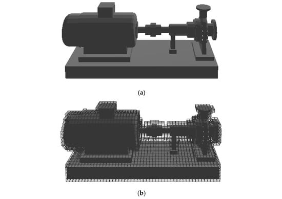
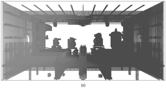
Figure 1.
Grid-based representation of ship equipment and hull structures. (a) Contour of the equipment; (b) Grid contour of the equipment; (c) Grid contour of the entire layout space.
Notably, the grid discretization can employ either uniform or non-uniform grids. Uniform grids result in an exponential increase in grid count as the space expands or grid size decreases. Non-uniform grids, such as those generated by the octree method [26,27], can significantly reduce grid counts in large spaces. However, non-uniform grids are less convenient for constraint representation and algorithm implementation. Since this paper focuses on the multi-objective A* algorithm and its comparative analysis, the uniform grid discretization is adopted. Future work will investigate its performance in non-uniform grid spaces. A smaller grid size improves routing precision but increases computational cost; thus, the grid size is typically set comparable to the diameter of the smaller pipes.
In a three-dimensional grid space, a pipe path P can be described by a sequence of grid cells from the starting point s to the endpoint t:
where a grid k is defined by the structure {idk, (xk, yk, zk), (rowk, columnk, layk), lengthk, bendk, energyk, violatek, pocketk}. Here, idk represents the grid marker; (xk, yk, zk) denotes the coordinates of the grid center point; and (rowk, columnk, layerk) indicates the indices of the grid in the spatial grid system. The remaining attributes describe evaluation quantities used for route optimization:
P = {grids, …, gridk, …, gridt}
- lengthk—represents the contribution of the grid k to the total pipe length;
- bendk—indicates whether a direction change (bend) occurs at the grid k;
- energyk—reflects the installation preference or difficulty of the grid k region, where a higher value implies less desirable routing space;
- violatek—records whether, at the grid k, the straight segment between two bends violates the minimum length constraint;
- pocketk—marks whether, at the grid k, a local “pocket” structure is formed between two vertical adjacent bends.
These attributes serve as auxiliary variables for computing the objective functions introduced in the following section and are used to evaluate the quality of each candidate pipe path in the multi-objective optimization process.
2.2.1. Objectives
- (1)
- Minimize pipe path length
The pipe path length should be as short as possible. The path length is calculated as the product of the grid edge length and the length of the grid sequence. This objective is expressed as:
- (2)
- Minimize pipe bends number
The bends in the ship pipe should be minimized. To determine whether a bend occurs at grid k, the vectors v1 (formed by the center points of grid k and its preceding grid k − 1) and v2 (formed by the center points of grid k and its succeeding grid k + 1) are analyzed. If the angle between v1 and v2 is not 180 degrees, a bend is formed. This objective is expressed as:
- (3)
- Minimize pipe energy (Preference for easy pipe installation areas)
The pipe energy should be as low as possible, favoring paths through grids with low energy values, which indicate areas where pipe installation is preferred. High-energy grids represent areas to avoid. The pipe energy objective is the summation of the energy values of the grids along the path, expressed as:
- (4)
- Ensure straight pipe segments between bends meet length constraints
The straight pipe segments between adjacent bends should not be shorter than the minimum required length (Lmin). If the distance between two adjacent bends is less than Lmin, a violation is counted. The algorithm works as follows: when bendk = bendt + 1, the first grid t with bend count bendk − 1 is identified in the sequence. If the distance between k and t is less than Lmin, the violation count is incremented. This objective is expressed as:
where violatek = 0 for non-bend grids, violatek = 1 if the bend grid violates the minimum length constraint, and violatek = 0 otherwise.
- (5)
- Avoid “pocket” structures in the pipe path
The pipe path should avoid forming “pocket” structure. For two adjacent bending grids k1 and k2, if the vector v1 (from grid k1 to grid k1 − 1) forms an angle less than 90 degrees with the z+ (vertical) axis, and the vector v2 (from grid k2 to grid k2 + 1) also forms an angle less than 90 degrees with the z+ (vertical) axis, the pipe segment between k1 and k2 forms a “pocket” structure with its adjacent segments. This objective is expressed as:
where pocketk = 0 for non-bend grids, pocketk = 1 if the bend grid forms a “pocket” structure with the previous adjacent bend grid, and pocketk = 0 otherwise.
Therefore, the multi-objective formulation for the SPRD in this paper can be described by Formula (10). It aims to achieve an optimal pipe layout that balances multiple competing objectives.
To facilitate the explanation of the algorithms and experimental results, the units of the main evaluation metrics used in this paper are specified in Table 2.
Table 2.
Definitions and units of main evaluation metrics.
2.2.2. Constraints
- (1)
- No collision between pipes, equipment, and ship structures
In the grid space, the occupied regions of equipment, structures, and pipes can be represented by their respective grid areas. To avoid collisions, the environmental objects are inflated based on the pipe diameter before routing a pipe. This inflation can be viewed as expanding the obstacle-occupied grid regions outward by n layers of grids, where the total thickness of the n layers is no less than half of the pipe diameter. In the grid space after the inflation, the algorithm only needs to search for the grid path that the pipe centerline passes through. Once the pathfinding is completed, the pipe can be expanded to its actual size along the centerline without colliding with the ship structures or the routed pipes. This preprocessing approach simplifies the algorithm implementation and enables the layout of pipes with different diameters within the same grid resolution. The number of inflation grid layers n can be calculated as follows:
where D denotes the diameter of the pipe, L denotes the side length of a grid, and floor() is a function used to round down to the nearest integer.
- (2)
- Orthogonal pipe routing with local non-orthogonal optimization
Orthogonal and straight pipe layouts are generally preferred in automated SPRD due to their advantages in space utilization and maintenance. However, because equipment interface orientations may not always be orthogonal, and certain local non-orthogonal pipe routes may better satisfy requirements like space savings and cost reduction, automated pipe design should prioritize orthogonal layouts while permitting non-orthogonal routing as a supplementary approach.
3. SPRD Based on MOA*
The Multi-objective A* (MOA*) algorithm is an extension of the classical A* algorithm designed to address path planning problems involving multiple optimization objectives. This paper proposes its application to the field of SPRD. Unlike the traditional single-objective A* algorithm, which focuses on minimizing a single cost function, the MOA* algorithm can consider multiple conflicting or independent objectives. Integrating heuristic search and multi-objective optimization, the MOA* algorithm efficiently produces Pareto-optimal solutions.
Previous bio-inspired multi-objective algorithms, which are based on population iteration and probabilistic mechanisms, are non-deterministic. In contrast, MOA* is a deterministic algorithm, offering advantages such as a solid theoretical foundation, flexible heuristic design, and adaptability to high-dimensional objective problems. It allows for controlled optimization strategies during path search, resulting in stable algorithm performance.
3.1. Multi-Objective A* Pipe Routing Framework
The pseudocode of the MOA* is presented as Algorithm 1, and the flow chart of the MOA* is depicted in Figure 2.
| Algorithm 1: MOA* |
Input:
Step 1. Initialization.
|
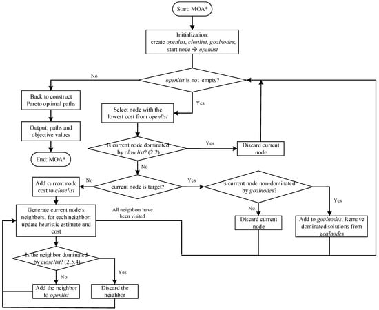
Figure 2.
The flow chart of the MOA* algorithm.
It may be noted that the standard MOA* algorithm directly performs dominance checks on the current node and its neighboring nodes during exploration. The dynamic probability-based pruning strategy proposed later uses the alternative steps. In Figure 2, the two boxes labeled 2.2 and 2.5.4 represent the standard steps of the MOA* algorithm. If the dynamic probability-based pruning strategy outlined in the pseudocode is adopted as an alternative, adjustments to these two boxes are required, as illustrated in Figure 3.
Figure 3.
Alternative flow charts for steps 2.2 and 2.5.4 in the MOA* algorithm.
Several key terms in the algorithm are briefly explained below.
The node in the algorithm has the following members. position: represents the node’s current location. g_cost: actual cost to reach the node. h_cost: heuristic cost to the goal. f_cost: total cost (g_cost + h_cost). parent_node: pointer to the parent node for path construction. direction: movement direction to reach the neighboring node.
The open list (openlist) and close list (closelist) are designed to manage nodes during the search. openlist: a priority queue that stores nodes to be explored, ordered by their total cost using a custom comparator, and ensures the most promising nodes are explored first. closelist: a hash map that stores non-dominated cost vectors for each visited position, using grid position as the key. It tracks explored nodes and their costs to avoid redundant exploration and maintain Pareto optimal solutions. goalnodes: a list stores the Pareto optimal paths that reach the target position. It keeps track of the non-dominated solutions at the goal (end_position) after the search process.
3.2. Time and Space Complexity
To evaluate the computational efficiency of the proposed MOA* routing algorithm, both theoretical and practical aspects of time and space complexity are analyzed. The following assumptions and notations are adopted for clarity.
Assumptions: (1) the routing space is discretized into grids with ; (2) each node expands to an average of m neighbors (6–26 directions, depending on whether non-orthogonal bends are allowed); (3) up to k non-dominated solutions are stored per grid cell; and (4) priority queue operations take . The probabilistic threshold only affects average pruning behavior, not the asymptotic bounds.
Time complexity: The worst-case time complexity is arising from node generations, queue operations, and dominance checks per exploration.
Space complexity: The memory consumption of the MOA* algorithm mainly comes from three components: (a) the discretized grid space, (b) the open list that stores nodes to be expanded, and (c) the close list that stores non-dominated solutions for each grid cell.
Let fcell the per-cell geometric and occupancy memory footprint, sobj the memory footprint of a single objective vector stored in the close list, and snode the average memory footprint of a node in the open list. The total memory consumption can be approximated as , where o is the maximum number of nodes in the open list and the close list (o n). Thus, the overall space complexity is upper-bounded by .
Practical scaling: Empirically, runtime grows roughly linearly with grid size n and branching factor m, and increases with k. However, obstacle density shows a non-monotonic effect, e.g., dense obstacles can sometimes reduce the number of explored nodes by shrinking accessible free space, but the exact impact depends on the spatial distribution of obstacles and may vary between cases. Allowing non-orthogonal neighbors (e.g., 135°) increases complexity but improves routing flexibility.
Practical limitations and mitigation: Since both computation and memory scale with n, fine-grained or large-scale pipe layouts may become inefficient. To address this, the cascade space expansion method (introduced later) first searches within a small region and only enlarges the search space when necessary, effectively balancing efficiency and scalability.
3.3. Cost Functions
In the proposed MOA* algorithm, the design of the cost functions primarily takes two forms, i.e., vector form and weighted sum form. Theoretically, the vector form is more commonly used for the cost function in the MOA* algorithm, as the comparison of solutions is based on dominance relationships among objectives. However, in the context of SPRD, using the vector form for the cost function results in lots of mutually non-dominated solutions in the open list, which can degrade the algorithm’s performance. In contrast, the weighted sum form addresses this issue. Therefore, one of the proposed methods employs the weighted sum approach for the design of open list comparator.
- (1)
- Vector form
Actual cost function: The costs of multiple objectives are represented as a vector.
Estimated cost function: Similarly, the heuristic values are represented as a vector.
Total cost function: The summation of the actual costs and estimated costs is represented as a vector.
- (2)
- Weighted sum form
Actual cost function: The costs of multiple objectives are weighted and summed to form a scalar value. For example,
where is the cost of the i-th objective, and is the corresponding weight.
Estimated cost function: Similarly, a weighted sum is used,
where is the heuristic estimate for the i-th objective.
Total cost function: The total estimated cost of node n is equal to the actual cost from the start node to node n plus the estimated cost from node n to the goal node.
Both forms have their advantages and disadvantages. The weighted sum approach is simple and easy to implement, but the selection of weights may influence the results. The vector form, on the other hand, can more comprehensively reflect the characteristics of multiple objectives, but it comes with higher computational complexity and may result in mutually non-dominated solutions during comparison. As illustrated in Figure 4, the vector dominance approach identifies a diverse set of Pareto-optimal solutions distributed across the Pareto front, whereas the weighted sum approach typically captures specific points determined by the selected weights. However, in practical applications, either form can be chosen based on the specific context, or both can be combined. Later experiments have shown that in the context of SPRD, the weighted sum method exhibits low sensitivity to weight selection, and assigning equal weights to all the sub-objectives can achieve satisfactory performance.
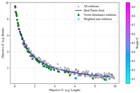
Figure 4.
Comparison between vector dominance and weighted sum.
For the heuristic function, the estimated values of the objectives only need to consider path length and bends number. This is because A*-like algorithms require that the estimated values of the objectives must not exceed the actual values (i.e., no overestimation) to ensure optimal solutions can be found. For the distance objective from the current node to the goal node, it can be estimated using the Manhattan or Euclidean distance. The bends number can be estimated by comparing the coordinates of the current node and the goal node across three dimensions (if the coordinates differ in any dimension, at least one bend is required, so the estimated number of bends ranges from 0 to 3). However, accurate lower-bound estimates cannot be provided for the other objectives, so they are simply set to 0. Thus, the heuristic function can be expressed as or .
3.4. Dominance Relationships for Pareto-Optimal Solutions
In the MOA* algorithm, node comparisons occur in several scenarios: (a) determining the dominance relationship between two nodes during exploration, (b) determining the dominance relationship between a node and its historical exploration records, and (c) determining the priority relationship between nodes in the exploration priority queue (open list) using a node comparator. Scenarios (a) and (b) are essentially the same.
If the cost function and heuristic function are designed based on the weighted sum of objectives, comparisons can be performed directly using the total cost values. If the cost function and heuristic function are represented in vector form, the dominance checking algorithm described in Section 2.1 is used.
For the node comparator in scenario (c), when using the weighted sum form, the total cost values can again be directly compared. However, when the cost is in vector form, two nodes may be mutually non-dominated. In this case, a deterministic tie-breaking rule is applied in our implementation. First, Pareto dominance is checked; if neither node dominates the other, a comparison is performed according to a predefined objective order (length, bend, energy, violation, pocket), and the node with a smaller value in the first differing objective is given higher priority. If two nodes have exactly identical cost vectors, the node inserted earlier is treated as having higher priority. This tie-breaking mechanism only affects the queue order among non-dominated nodes and preserves the admissibility and consistency required for obtaining Pareto-optimal solutions.
3.5. Dynamic Probability-Based Pruning Strategy
Bio-inspired multi-objective search algorithms (e.g., MOACO, NSGA-II) do not impose layout constraints during the exploration phase of generating individuals, allowing path exploration to span the entire layout space. Subsequently, the objective vectors of the individuals are calculated and compared to determine their quality. In contrast, the MOA* algorithm evaluates the superiority of newly added nodes (based on the cost value, which includes objectives such as length and bends) during the generation of paths. Nodes deemed non-superior are pruned, which can lead to insufficient exploration of the search space. The nodes pruning explains why MOA* usually finds fewer solutions than bio-inspired algorithms. To address this issue, an improved strategy is proposed to relax the restrictions on new nodes added to the open list, enabling the algorithm to explore more possibilities.
This paper introduces a dynamic probability-based pruning strategy. In the standard MOA*, when selecting the next node to expand from the open list or adding new neighboring node to the open list, the algorithm compares the node’s objective costs with the historical Pareto-optimal solutions recorded in the close list. The node is only processed if it is not dominated by the historical optimal solutions; otherwise, it is skipped. As mentioned earlier, this approach may prematurely prune nodes that appear unpromising at the current stage but have potential in later stages, leading to a reduction in the number of optimal solutions. The new strategy calculates a dynamic probability threshold σ. Each time a node is processed (either popped from or added to the open list), if a randomly generated probability is less than σ, the node is processed without dominance comparison. If the probability is not less than σ, the node is processed only if it is not dominated. This approach effectively balances exploration and exploitation, enhancing the algorithm’s ability to discover more solutions while maintaining computational efficiency. Moreover, as the new strategy represents a more relaxed version of the standard MOA* pruning rule, it still preserves the admissibility and consistency required for obtaining Pareto-optimal solutions.
The selection of the threshold σ is crucial. If σ is too large, too many nodes are expanded, significantly reducing the algorithm’s efficiency. If σ is too small, insufficient nodes are expanded, degrading the algorithm’s optimization capability. To address this, a dynamic threshold is proposed. σ is calculated as follows:
where n is the count of nodes popped from the open list, and b is the total number of grids in the layout space. The value of σ decreases from nearly 1 to nearly 0 as the number of explored nodes n increases. When n = b, σ(n) = 0.5. Before n reaches b, even nodes that are not currently optimal have a higher probability of being explored. After n exceeds b, the pruning probability becomes stricter to ensure convergence of the search process. Additionally, a tuning coefficient a can be introduced to further control the decay rate by multiplying (n − b). However, in ship pipe routing cases, setting a = 1 generally yields satisfactory results. The schematic diagram of σ(n) is illustrated in Figure 5.
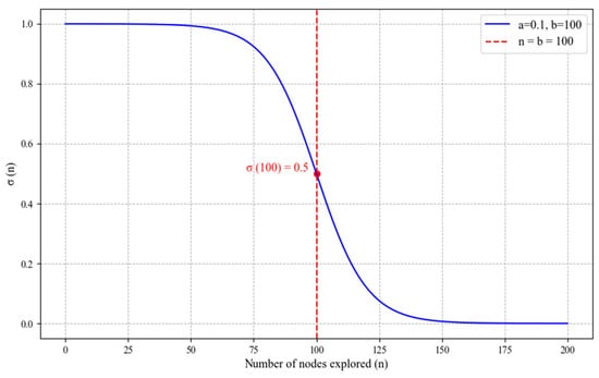
Figure 5.
Function curve of σ(n).
The dynamic probability-based pruning strategy is implemented in steps 2.2 [Alternative] and 2.5.4 [Alternative] of the MOA*. Unlike the standard MOA* algorithm, which performs dominance comparisons for all nodes, this strategy determines whether to perform dominance comparisons based on a dynamic probability threshold.
3.6. Neighbor Node Exploration and Non-Orthogonal Piping
In actual ship pipe engineering, besides 90-degree bends or elbows, common bending angles also include 120 degrees, 135 degrees, and 150 degrees. However, current research on algorithm-based piping primarily employs orthogonal piping (90-degree bends). The main reasons are firstly, the layout obtained through orthogonal piping, though possibly not optimal, are feasible; secondly, permitting more bending angles increases the complexity of the algorithm and necessitates handling more exceptional cases (e.g., unreasonable bending angles, excessive non-orthogonal scenarios making installation difficult). The proposed MOA* algorithm can support non-orthogonal pipe path to a certain extent. By setting the exploration directions of neighbor nodes, it can generate a wider variety of paths. In step 2.5 of the MOA* algorithm, it explores the non-obstacle neighbor nodes around the current node. If considering the neighbors in the orthogonal directions of the current node’s faces, there are 6 directions: East (“E”), West (“W”), South (“S”), North (“N”), Up (“U”), and Down (“D”). If considering the neighbors in the diagonal directions of the current node’s edges, there are an additional 12 directions: (“NE”, “SE”, “NW”, “SW”, “EU”, “ED”, “WU”, “WD”, “NU”, “ND”, “SU”, “SD”). If further considering the neighbors in the diagonal directions of the current node’s vertexes, there are another 8 directions: (“NEU”, “NED”, “SEU”, “SED”, “NWU”, “NWD”, “SWU”, “SWD”). The schematic diagram of the positional relationships between nodes is shown in Figure 6. Clearly, as the exploration directions increases, the search space expands dramatically, and the excessive complexity can render the routing algorithm impractical.
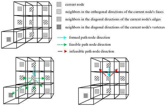
Figure 6.
The schematic diagram of the positional relationships between neighboring nodes.
Therefore, the following recommendations are made: for most pipes, orthogonal directions should be used to explore neighboring nodes, ensuring a clear and regular layout. For pipes where minimizing path length is more critical than maintaining orthogonality, it is advisable to allow limited non-orthogonal exploration. When the search space is large, 1 to 4 additional non-orthogonal directions can be introduced to improve routing flexibility. In practical ship piping design, moderate non-orthogonal bends—typically around 135°—can be adopted in appropriate cases to balance routing flexibility and installation feasibility while reducing excessive detours. Compared with sharp 90° turns, 135° bends can, when applicable, alleviate local flow resistance and stress concentration, promoting smoother fluid transition and easier installation within confined compartments.
A constraint can be added in step 2.5.1 of the MOA* to ensure that the bending angle formed between a new neighboring node and adjacent path node is not acute, thereby skipping the exploration of such undesirable nodes; in engineering, a stop control variable can be added in step 2 of the MOA* to support software UI operation to abandon a complete search.
3.7. Cascade Space Expansion Method
The efficiency of the MOA* algorithm is directly related to the scale of the search grid space. In SPRD, the number of pipes is substantial, and exploring the entire space for each pipe would be computationally expensive. This is because the pipe path connecting interfaces typically does not span the entire space but is usually confined to a specific spatial region. To enhance efficiency, a cascade space expansion approach is proposed. Initially, a bounding box space containing the interfaces or branch points is constructed and slightly expanded to serve as the initial search space. If the algorithm fails to find feasible pipe paths within this space, the space is expanded by a ratio. This process continues until the MOA* algorithm obtains a solution or reaches the threshold of iterations. Each generated space must undergo an intersection operation with the entire layout space to ensure the validity of the search space. The algorithmic workflow is described as Algorithm 2. Figure 7 demonstrates how the cascade space expansion method constructs paths between interfaces across a partition.
| Algorithm 2: Cascade space expansion |
Input:
Step 1. Set parameters.
|
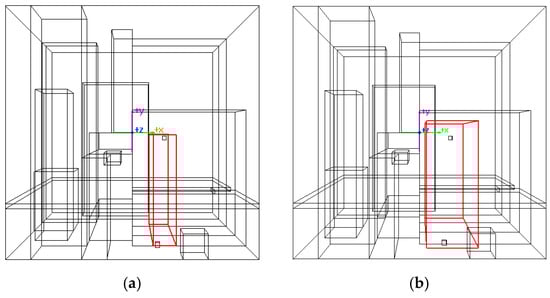
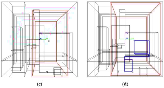
Figure 7.
Example of pipe routing via the cascade space expansion. (a) The 1st attempt; (b) The 2nd attempt; (c) The 3rd attempt; (d) The 4th attempt.
4. Experiments and Results
4.1. Configuration
Unlike bio-inspired algorithms that require the setting of many hyperparameters, the standard MOA* does not require any hyperparameters. The probability-based pruning version requires only two parameters, a and b, where setting a = 1 typically yields satisfactory results, while b is directly set to the spatial grid count. Once configured, these parameters do not require further adjustment. In the case of weighted sum cost functions, uniform weights (i.e., 1.0) are assigned to each objective. Conversely, when using vector-form cost functions, Pareto dominance is evaluated based solely on the objectives, obviating the need for weight assignment. Therefore, compared to previous multi-objective algorithms, the proposed algorithm significantly reduces the demand for user expertise. For exploring neighbor nodes, the algorithm uses 6 orthogonal directions as its default setting. Unless otherwise specified, the parameter settings used in the subsequent experiments follow the configuration described here, and only adjusted parameters and settings are explicitly stated.
Software development and runtime environment: Windows 11 x64, Visual Studio 2022, C++ optimization set to prioritize speed (/O2), OpenGL 10.0; CPU: 12th Gen Intel(R) Core (TM) i7-12700H 2.30 GHz, RAM: 32 GB, SSD: 1 TB.
4.2. A Simulation Piping Case
The environment for the case study is a cubic space of 100 mm 100 mm 100 mm, with the center of the space as the origin. Inside this space, there are 22 rectangular obstacles, and their diagonal positions are shown in Table 3. To compare the MOA* with the previous multi-objective algorithms [13,14], the space is divided into 50 50 50 grids, the grid energy near the obstacles, floors and walls is set to 0, with other settings detailed in [13,14]. There are two pipes to be routed, with their start and end grid positions (i.e., row, column, layer) as follows: P1: (49, 0, 49)~(49, 23, 0), P2: (49, 0, 49)~(0, 40, 0).
Table 3.
Obstacle positions.
- (1)
- Experiment 1: Performance evaluation under different algorithm settings
This experiment aims to compare the performance of different algorithm settings, utilizing the entire space as the search area. Based on the forms of the cost functions, as well as the pruning strategy for nodes exploration, the MOA* algorithms are divided into four types. _weight denotes the use of weighted sum form for cost functions, _vector denotes the use of vector form for cost functions, and _dynamic denotes the use of a probability-based pruning strategy for historical dominance comparison of nodes; otherwise, all nodes undergo historical dominance comparison. Since the two _dynamic MOA* variants based on the probability-based pruning strategy involve randomness, while the other two are deterministic, four layout spaces with progressively increasing obstacle density and distribution complexity were designed to ensure a more objective assessment of the algorithms’ performance. In each layout, two pipes with significantly different routing orientations were selected to conduct validation experiments. The experimental results are shown in Table 4. Since the algorithms produce a large number of Pareto-pattern solutions that are mutually non-dominated, it is not feasible to list the detailed indicator values for all patterns in the tables due to space limitations. Therefore, most of the experimental tables present only the comparison of the number of patterns, while specific indicator values are provided only for the representative optimal solutions and the statistical results.
Table 4.
Data results of MOA* under different settings.
From the consistent trends observed in the results presented in Table 4, the main conclusions can be summarized as follows.
- (1)
- MOA*_weight_dynamic and MOA*_vector_dynamic, which incorporate a dynamic probability-based pruning strategy, yield a greater number of Pareto-optimal solutions across different obstacle distributions compared to their counterparts without the strategy (P2 is more obvious). However, the dynamic strategy does not enhance the number of Pareto patterns. This approach loosens early-stage pruning constraints, allowing the algorithm to retain initially suboptimal nodes that may become advantageous. Consequently, as the algorithm explores more nodes, the search duration is extended accordingly.
- (2)
- A comparison between MOA_weight_dynamic and MOA_vector_dynamic, as well as between MOA_weight and MOA_vector, reveals that algorithms using the weighted sum cost functions exhibit slightly better performance than their vector-based counterparts. The primary reason lies in the design of the comparator in the MOA* open list. In the vector-based method, there are many cases of mutual non-dominance solutions, which complicates the priority comparation. In contrast, the weighted sum method does not encounter this issue. Overall, when balancing the algorithm’s optimization and time performance, MOA*_weight_dynamic holds a slight advantage.
Figure 8 illustrates the layouts of P1 and P2 under various obstacle distributions after one run of MOA*_weight_dynamic. The data depicted in Figure 8 is as shown in Table 5. The MOA* algorithms can provide Pareto optimal solutions, offering valuable references for engineers.
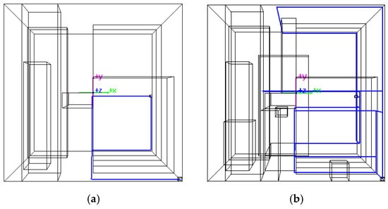
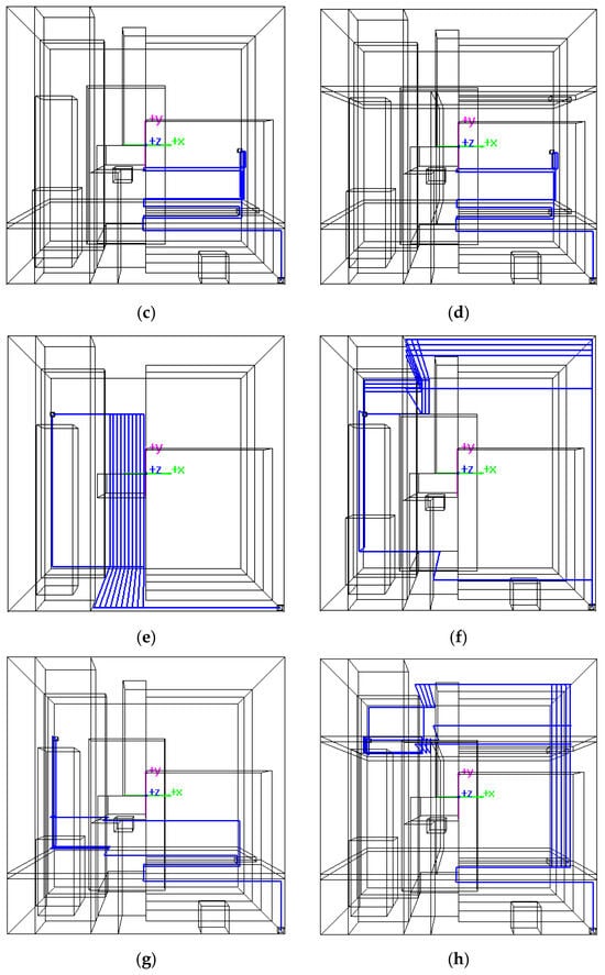
Figure 8.
Layout of the Pareto optimal solutions for case 1 (MOA*_weight_dynamic, P1 and P2). (a) P1, 6 obstacles, pareto num. 2, pattern num. 1; (b) P1, 13 obstacles, pareto num. 16, pattern num. 5; (c) P1, 17 obstacles, pareto num. 5, pattern num. 1; (d) P1, 22 obstacles, pareto num. 4, pattern num. 1; (e) P2, 6 obstacles, pareto num. 20, pattern num. 1; (f) P2, 13 obstacles, pareto num. 15, pattern num. 6; (g) P2, 17 obstacles, pareto num. 6, pattern num. 1; (h) P2, 22 obstacles, pareto num. 39, pattern num. 9.
Table 5.
Data results corresponding to Figure 8.
- (2)
- Experiment 2: Sensitivity analysis of weight settings in MOA*_weight
In the above experiment, both MOA_weight and MOA_weight_dynamic achieved satisfactory results with all weights in cost functions set to 1. In the following experiment, MOA_weight is chosen as the representative algorithm. Some weights are adjusted in the space with 13 obstacles to observe the performance in routing P1 and P2. The weights were kept in their original scale (without normalization) for intuitive comparison. As MOA_weight is deterministic, only one execution is needed for each setting. The results are shown in Table 6.
Table 6.
Weights effect comparison in MOA*_weight (13 obstacles).
Analysis of the table data shows that the number of nodes explored by the algorithm may vary under different weight settings, potentially leading to different Pareto optimal solutions. This is consistent with A* algorithm’s principle of relying on cost functions for pathfinding. Furthermore, the experiment demonstrates that the MOA* for SPRD, using a weighted sum as the cost function, is not highly sensitive to weight settings in discovering optimal solutions. A key metric of the algorithm, the number of Pareto patterns, remained stable despite weight adjustments, indicating strong robustness and reducing parameter tuning requirements.
- (3)
- Experiment 3: Comparative analysis of search directions in MOA*
The results of the A* algorithm are related to the search direction primarily due to the asymmetry of the heuristic function, the non-uniform distribution of obstacles, and the dependency of node expansion sequence. Taking MOA*_weight and MOA*_vector as instances, the impact of pathfinding direction on the MOA* algorithms is verified by swapping the start and end grids of P1 and P2, resulting in two pipes P1*: (49, 23, 0)~(49, 0, 49) and P2*: (0, 40, 0)~(49, 0, 49). The results after one execution of the algorithms are shown in Table 7.
Table 7.
Routing results of swapping start and end interfaces.
A comparison of the MOA*_weight and MOA*_vector data in Table 7 with their counterparts in Table 4 reveals that for pipes P1 and P1*, P2 and P2*, which share identical interface positions but have their start and end swapped, the number of Pareto optimal solutions and patterns obtained by the same algorithm varies significantly. Additionally, the runtime nearly doubles. This discrepancy mainly arises because the distribution of obstacles and the positions of interfaces are asymmetric, influencing the final layouts. A key insight from this experiment is that when employing the MOA* algorithm, initiating the search from different directions may help uncover more optimal solutions.
- (4)
- Experiment 4: MOA* vs. bio-inspired multi-objective algorithms
In the following experiment, MOA*_weight_dynamic is compared with the MOACO and NSGA-II algorithms, all executed under the same hardware environment. To ensure a fair comparison, the number of iterative generations for both MOACO and NSGA-II is set to 100, and other algorithm parameters are configured according to the best settings reported in studies [13,14]. Both MOACO and NSGA-II contain multiple algorithmic and framework-level hyperparameters that require careful tuning to achieve satisfactory performance. In contrast, the proposed MOA algorithm involves only a few hyperparameters, as described in Section 4.1, making it easier to configure and more robust across different problem settings. Because the algorithms are non-deterministic, we perform five runs for each obstacle configuration to ensure reliable comparisons. The mean and standard deviation (SD) of the results are shown in Table 8.
Table 8.
Comparison of results from three multi-objective algorithms (* marked results indicate premature termination).
The data shows that the MOA* algorithm sometimes finds fewer Pareto-optimal solutions than the bio-inspired algorithms (e.g., with 17 and 22 obstacles) but produces more diverse solution patterns. Crucially, in complex obstacle distributions, it reliably finds a path when one exists, and both mean and standard deviation metrics demonstrate its clear superiority over bio-inspired approaches. As the number of obstacles increases, the MOA* algorithm explores fewer nodes, leading to higher efficiency. In practical applications, the number of pipe routing patterns formed by objectives is more important to users than the number of Pareto-optimal solutions. This is because different Pareto solutions within the same pattern exhibit minimal differences, and an excessive number of solutions can burden users with decision-making. The MOA* algorithm demonstrates superior performance due to its diverse routing patterns and stable performance.
The weakness of the MOACO lies in the decreased success rate of its heuristic pathfinding algorithm in complex space, which necessitates repeated attempts and significantly increases the time for pipe routing. In some cases, the algorithm may even exceed the pathfinding retry threshold. For instance, in the case of the P2 pipe with 22 obstacles, all five iterations were terminated prematurely at the 29th, 9th, 22nd, 13th, and 20th generations, respectively. Thus, its statistical results are marked with an asterisk (*).
In contrast, the NSGA-II introduces a randomly positioned intermediate connection point and constructs paths using the A* algorithm based on the pipe’s starting point, the connection point, and the end point. Although pathfinding may fail when the connection point is in an enclosed space, the pathfinding capability of the A* ensures success upon regenerating new connection points. However, this strategy reduces the algorithm’s efficiency.
- (5)
- Experiment 5: Validation of non-orthogonal and partial exploration scenarios
As mentioned in the previous section, when the MOA* allows exploration of non-orthogonal neighbors, it can generate non-orthogonal pipe routes. This is particularly feasible for pipes where length is prioritized over orthogonality. Figure 9 illustrate the layout of pipe P2 in a space with 17 obstacles, with exploration enabled in both 6 orthogonal directions and the “NU”, “ND”, “SU”, “SD” directions. Figure 9a displays all Pareto-optimal solutions, while Figure 9b showcases a selected layout. It is evident that non-orthogonal routing can reduce pipe length but increase installation complexity. Users can decide whether to enable this feature based on their requirements.
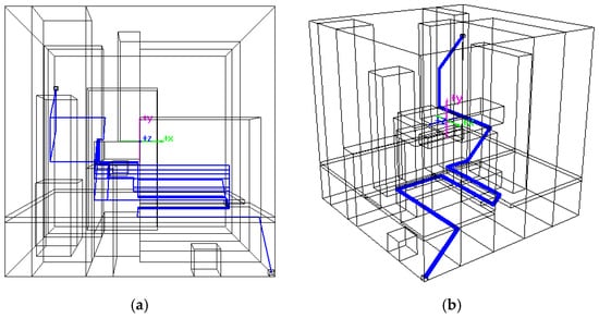
Figure 9.
Layout with non-orthogonal routing. (a) Pareto optimal solutions; (b) a user selected solution.
The search time of the MOA* is proportional to the number of nodes traversed. If speed is prioritized over obtaining all optimal solutions, the algorithm can be terminated early to obtain partial optimal solutions. For example, an observation-based method can be employed: when the explored grids cover most of the space between the pipe’s start and end points, the algorithm can be manually terminated. Upon detecting the termination signal, the algorithm ceases to explore new nodes. In most cases, the solutions are sufficient to meet the requirements. Figure 10 illustrates the comparison between partial and full exploration of nodes in the space (obstacles occupied spaces are not explored).
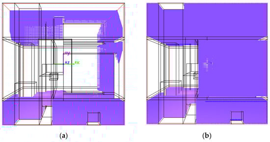
Figure 10.
Partial and full exploration of nodes. (a) Partial exploration; (b) full exploration.
4.3. A Fuel Piping Case in Engine Room
The experiment was conducted on the fuel piping system of a ship’s engine room, as described in [11]. The space contains 3 daily fuel tanks, 1 steam boiler, 1 hot water boiler, 2 diesel generators, 1 main engine, and 2 fuel transfer pumps. The layout space encompassing all equipment measures 10,000 mm × 4000 mm × 6000 mm. The design requires the layout of 8 fuel pipes (P1–P8) connecting the equipment. Detailed configuration of the equipment models, pipe interface locations, and dimensions can be found in [11]. The pipe schematic is shown in Figure 11, where P1, P6, P7, and P8 are branched pipes, and P2, P3, P4, and P5 are single pipes. The original CAD model is shown as Figure 12. The grid size is set to 50 mm based on the minimum pipe diameter size. In the actual pipe engineering, to improve efficiency, the entire space is not used as the search space. Instead, the space cascaded expansion method proposed in Section 3.7 is employed. The initial space for each pipe or branch is a cuboid enveloping the terminals to be connected. When the MOA* algorithm fails to find a valid path, the space is automatically expanded. In this study, the expansion coefficient is set to 1.5. The extension distances of pipe interfaces, grid energy distribution, and pipe arrangement order are kept consistent with those in [11,14]. For ease of installation, pipes P6 and P7 extend 7 and 4 grid distances, respectively, at the lower interfaces of the daily fuel tanks, while the remaining interfaces extend 2 grid distances. The pipes are arranged in the order of P1, P4, P5, P3, P2, P6, P7, and P8. The order of branches within the pipes is arranged from the largest to the smallest diameter. To enhance efficiency, the connection points of branches are automatically selected based on distance, i.e., the nearest grid on the routed branch to the target interface is selected as the connection point. For fair comparison, this study maintains the envelope bounding box method for equipment modeling as previous works. This case study employs the MOA*_weight_dynamic variant for the comparative experiments, with the weight and other parameter settings described in Section 4.1.
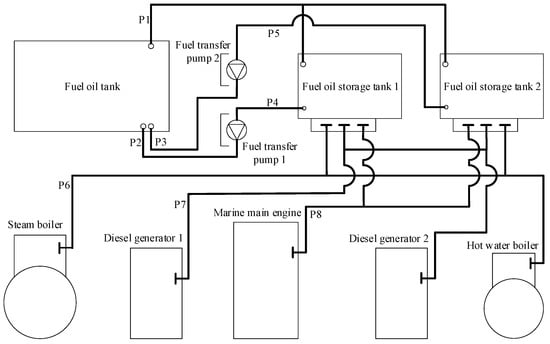
Figure 11.
The pipe schematic diagram.
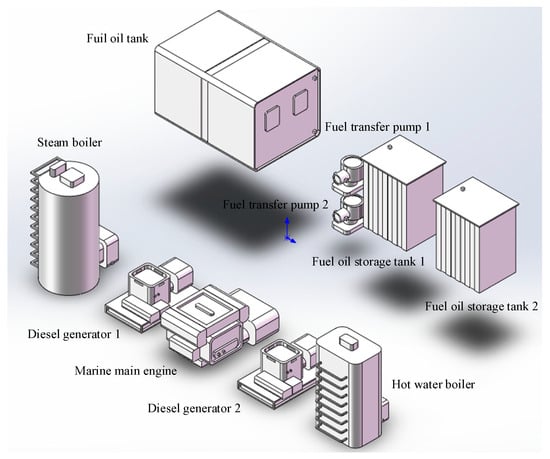
Figure 12.
The CAD model of the fuel piping equipment.
- (1)
- Experiment 1: Performance benchmarking of MOA* against prior bio-inspired algorithms
First, the grid energy is initially set to 0, thereby excluding the path energy objective from searching. When energy is not considered, the pipe layout design prioritizes straight pipe runs and minimal bends over proximity to the floor or equipment surfaces. The routing results are shown in Figure 13.
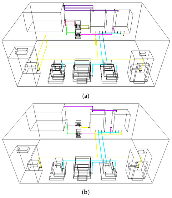
Figure 13.
The routing effects of MOA* that ignores the path energy objective. (a) Pareto optimal pipe routings; (b) one selected optimal pipe routing.
If the energy objective is considered, the pipes can be prioritized to pass through low-energy regions. For example, only the grids close to equipment and floor are set to energy value of 0. The routing results are shown in Figure 14.
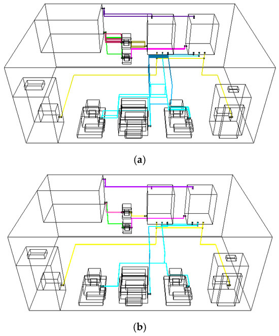
Figure 14.
The routing effects of MOA* that considers the path energy objective. (a) Pareto optimal pipe routings; (b) one selected optimal pipe routing.
A comparison with the results of the MOACO [14] and GA-A* [11] algorithms is shown in Table 9. The data include the pipe and branch lengths (L), number of bends (B), number of branch points (R), energy values (E), and runtime cost (T) for each pipe. All solutions meet the requirements for straight-pipe segment limit and no “pocket” structures, so these are not listed in the table. When the algorithms do not consider grid energy, the energy value (E) in the results is marked as NA.
Table 9.
Routing results of the fuel piping system using multiple algorithms.
It may be noted that the comparison is based on the same practical engine-room routing case, where the MOACO and GA-A* reported the optimized layouts under their best parameter settings. As MOACO (multi-objective evolutionary), GA-A* (hybrid), and MOA* (deterministic search) differ greatly in algorithmic principles, the experiments were not unified under identical iterative generations or implemented in the same computing environment. The comparison mainly focuses on the routing quality indicators corresponding to the best experimental results, including pipe length, number of bends, branch points, and energy value.
For reference, the hardware environments used in the respective studies are as follows: GA-A*—Intel i5-7500 CPU 3.40 GHz; MOACO—Intel i5-8265U CPU (base 1.60 GHz, up to 3.90 GHz); and MOA*—Intel i7-12700H CPU (base 2.30 GHz, up to 4.70 GHz). All experiments were executed with sufficient memory, and the latter two processors are mobile platforms whose frequencies may fluctuate during runtime.
From the comparison of the Total data in the table, it can be observed that the MOA* algorithm improves the metrics for all eight pipes in terms of pipe length, bends number, and runtime when grid energy is not considered, while the number of branch points remains the same. When grid energy is considered, only the grid energy metric is slightly higher due to the cascaded spatial expansion limiting the initial search space. The number of branch points remains unchanged, while all other metrics show improvement. Referring to the Total data, compared to the MOACO algorithm, which previously demonstrated better performance, the total pipe length is reduced by 7.2% and 6.6%, and the total bends number is reduced by 6.8% and 9.3% for cases with and without energy, respectively. Analysis of the data reveals that the MOA* algorithm, when routing pipes 6 and 7, can identify layouts that allow for more shared paths between branches, resulting in shorter pipe lengths and fewer bends.
In terms of computational efficiency, the MOA* algorithm reduces runtime by 74.5% and 89.8% compared with the MOACO, and by 92.5% and 96.9% compared with the GA-A*, for cases with and without energy, respectively. It should be noted that the runtime comparison is indicative rather than strictly quantitative, as the experiments were performed on different hardware platforms. Nonetheless, the results clearly demonstrate that the proposed MOA* achieves an order-of-magnitude advantage in computation time while maintaining superior routing quality. Moreover, the proposed algorithm requires no parameter tuning, making it convenient and robust for practical applications.
In Table 10, the number of Pareto optimal solutions and patterns for each pipe and its branches under energy-considered and energy-ignored scenarios is shown. As analyzed in Case 1, the MOA*_weight_dynamic algorithm employs a probability-based pruning strategy, introducing randomness in the results. Moreover, in multiple pipes routing, the choice of optimal solutions for earlier pipes influences the routing space for subsequent pipes, resulting in different solutions for the latter. Thus, the data in Table 9 and Table 10 reflect optimal solutions from a single run and do not represent the global optima.
Table 10.
Pareto optimal solution number and pattern number of each pipe.
Although automated routing algorithms can generate preliminary layout designs, manual adjustments are still necessary when design constraints are not fully incorporated. For instance, the routing algorithm connects branches based on the shortest distance, ignoring the flow requirements. Thus, in Figure 13 and Figure 14, P6 and P7 share branch paths to the greatest extent possible. If the branch pipe diameters are insufficient, it can be addressed by increasing the sub-branch diameter or connecting the sub-branch to main branch.
- (2)
- Experiment 2: Attraction zone-based pipe routing
In practical piping, low-energy zones can be defined to attract pipes with close interfaces, enabling compact layouts for easier installation or more workspace. For example, Figure 15 shows the layout after setting a low-energy zone in the 6-to-11-layer grids. Most branches of pipes P6, P7, and P8 passing through this zone are concentrated, which mitigates the issue of dispersed branch layouts in large spaces.
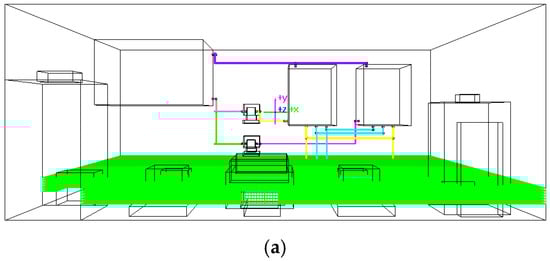
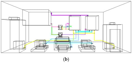
Figure 15.
The routing effects of MOA* that sets a low-energy zone. (a) The low-energy zone; (b) concentrated pipe layout in the low-energy zone.
- (3)
- Experiment 3: Non-orthogonal routing validation for ship fuel piping system
In this experiment, without considering grid energy, the MOA*_weight_dynamic algorithm is allowed to explore nodes in both orthogonal and horizontal diagonal directions (“EU”, “ED”) during pathfinding. The Pareto optimal paths are shown in Figure 16, revealing the presence of 135-degree bends. Figure 17a illustrates the user-selected layout from Figure 16 integrated into the original CAD model. Compared to the orthogonal pipe layout in Figure 17b generated by the same algorithm, the non-orthogonal configuration reduces total pipe length by 1300 mm but requires 9 additional bends and increases runtime by approximately 68 s. To mitigate the complexity introduced by non-orthogonal directions, a constraint can be added in step 2.5.1 of the MOA* to ensure that the bending angle formed between the new neighboring node and its adjacent predecessor node is not acute. If the angle is acute, this neighbor is discarded. After this change, the performance improves by approximately 10%. When installation conditions allow, non-orthogonal pipe design can shorten the pipe length and save workspace, consistent with the rationale behind manual piping practices.
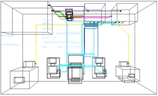
Figure 16.
Pareto optimal solutions of non-orthogonal pathfinding for pipe route design.
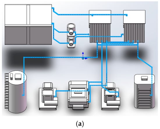
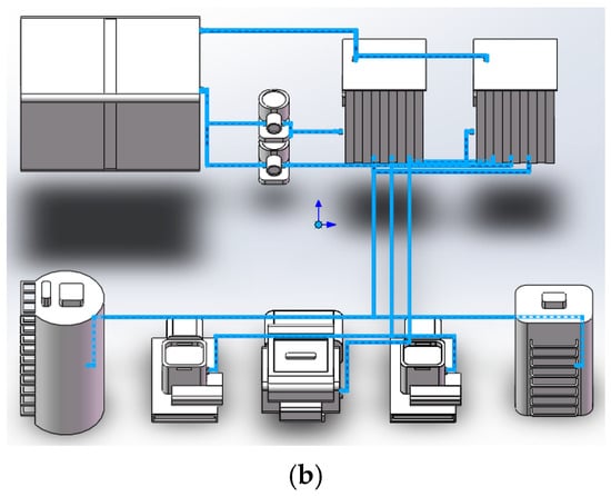
Figure 17.
Comparison between partial orthogonal and fully orthogonal pipe layouts. (a) LTotal = 52,850 mm, BTotal = 38, RTotal = 6, TTotal = 78,039 ms; (b) LTotal = 54,150 mm, BTotal = 29, RTotal = 6, TTotal = 10,485 ms.
4.4. A Complex Piping Case in System Compartment
As the ultimate benchmark, the MOA_weight_dynamic and MOA_vector variants with parameter settings described in Section 4.1, together with the comparative algorithms NSGA-II and MOACO, were tested against the complex ship pipe routing case established in [8]. To balance solution quality and computational efficiency, both NSGA-II and MOACO were configured with 20 iterative generations, and other parameters followed the best practices reported in [13,14]. The case defines a rectangular space of 3080 mm × 4860 mm × 2340 mm containing all the pipe interfaces, within which hull structures, equipment, five pipes to be routed, and a virtual workspace to be avoided exist. The pipe configurations are as follows: Pipe 1 (9 interfaces), Pipe 2 (7 interfaces), Pipe 3 (2 interfaces), Pipe 4 (8 interfaces), and Pipe 5 (5 interfaces). Detailed interface specifications (positions, orientations, diameters, initial extension distances, and connected equipment/hull penetrations) are provided in [8]. The space was discretized using 20 mm cubic grids considering pipe diameters and installation clearances.
Unlike previous studies that used bounding boxes to model equipment, which compromises accuracy and efficiency. This case study directly initializes the routing space by marking grids intersected by the triangular mesh contours of equipment and hull structures from STL files as obstacles.
To address the SPRD problem, the authors’ team developed a three-dimensional ship pipe route design software based on C++ and OpenGL technologies, integrating various design algorithms. The spatial meshing effect of the STL model and the interfaces for this case study are shown in Figure 18.
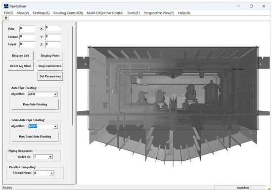
Figure 18.
Visualization of the layout space within the software.
Since the five pipes were routed sequentially, each pipe or branch could generate multiple Pareto-optimal solutions. The selection of different solutions consequently influenced the layout environment for subsequent pipelines. Moreover, the routing algorithms themselves involve a certain degree of stochasticity. Therefore, each algorithm was executed five times, and the mean and standard deviation (SD) of the obtained results were calculated, as presented in Table 11.
Table 11.
Comparison of results from different pipe routing algorithms.
It is worth noting that the MOA* variants enabled the “NE” and “SE” directions in non-orthogonal layouts. For all layout solutions produced by the compared algorithms, the minimum straight pipe segment constraint (i.e., no less than three times the pipe diameter) was satisfied, and no “pocket” structures were formed in the vertical direction. Consequently, only four comparative indicators are reported in Table 11.
The results in Table 11 lead to several key findings:
- (1)
- In the orthogonal routing case, NSGA-II achieved the shortest average pipe length and, together with MOA*_weight_dynamic, yielded the smallest count of bends. It also exhibited relatively low memory consumption. However, the algorithm required significantly longer computation time than the others.
- (2)
- MOACO performed the worst in orthogonal routing, generating the longest pipelines and the highest count of bends. Nevertheless, it demonstrated the lowest memory consumption and much shorter computation time compared with NSGA-II, though its overall performance was still inferior to that of the MOA* variants.
- (3)
- MOA*_weight_dynamic produced slightly longer pipe lengths than NSGA-II but with smaller standard deviations and also the best performance in terms of the count of bends. It showed a clear advantage in computation time while incurring only a minor increase in memory usage relative to NSGA-II and MOACO.
- (4)
- MOA*_vector exhibited balanced performance in orthogonal routing. Its results for pipe length, count of bends, and memory consumption were moderate, but it achieved the shortest computation time among all tested algorithms.
- (5)
- In the non-orthogonal routing scenario, MOA*_weight_dynamic was slightly inferior to MOA*_vector in pipe length and count of bends but outperformed it considerably in computation time and memory usage.
Based on these findings, the following recommendations are proposed for the practical algorithm selection:
- (1)
- The MOA* variants are preferable. Among them, MOA*_weight_dynamic demonstrates the most balanced overall performance, while MOA*_vector is particularly suitable for orthogonal routing scenarios where computational efficiency is a primary concern.
- (2)
- When computation time is not a limiting factor, NSGA-II or MOACO may also be adopted. Increasing the number of iterative generations or iterations can potentially improve the solution quality.
- (3)
- For non-orthogonal routing, it is advisable to enable only limited (1–4) additional 135° directions based on specific design requirements. Activating more non-orthogonal directions will significantly increase the number of explored nodes, leading to a sharp rise in the spatiotemporal complexity of the MOA* variants.
In addition, the optimal layout reported in [8] achieved a total pipe length of 58,160 mm with 68 bends. In contrast, the improved MOA* variants proposed in this study produced several solutions that outperform these metrics. Figure 19a,b illustrate orthogonal routing results, which are superior to those presented in [8], while Figure 19c,d show non-orthogonal routing solutions obtained by enabling the orthogonal “NE” and “SE” directions.
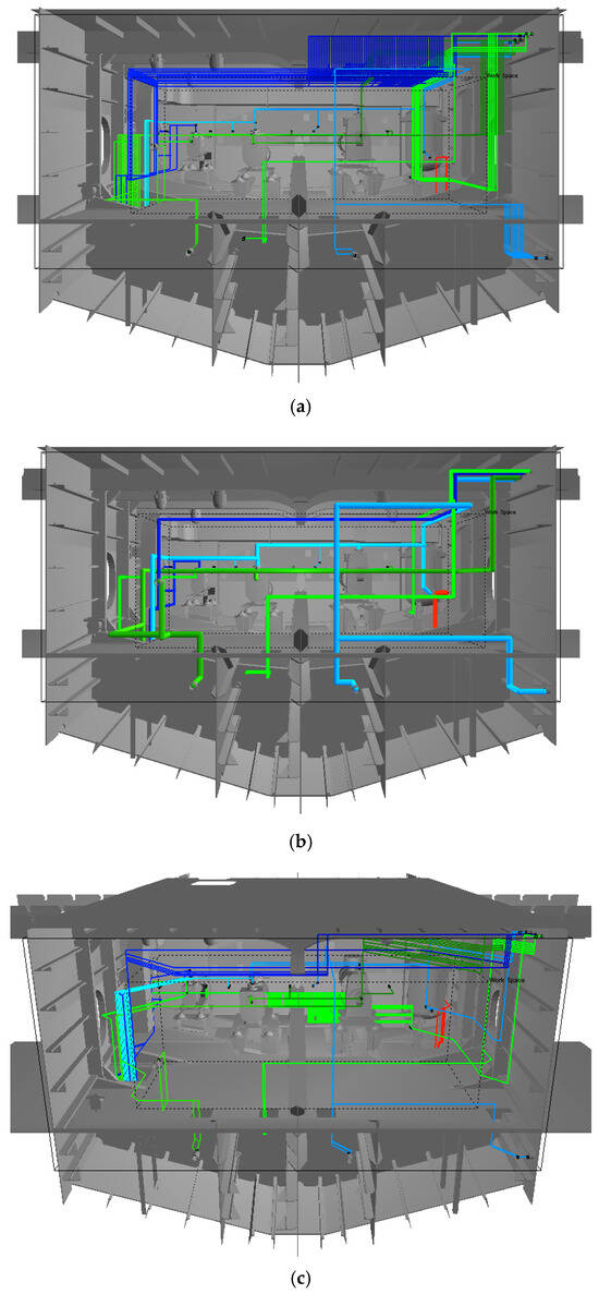
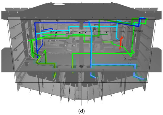
Figure 19.
The optimized layout results. (a) Pareto optimal solutions (orthogonal); (b) a user selected layout (orthogonal, length = 58,060 mm, bends = 67); (c) Pareto optimal solutions (partial orthogonal); (d) a user selected layout (partial orthogonal, length = 52,220 mm, bends = 72).
The experimental results confirm that our method delivers diversified routing layouts through multi-objective optimization, demonstrating advantages in several typical scenarios.
5. Conclusions
In this paper, we introduce MOA* algorithms to solve the SPRD problem. Unlike the conventional evolutionary or swarm-based multi-objective algorithms that require substantial hyperparameter tuning, MOA* offers a deterministic, non-iterative approach with significantly reduced parameter tuning demands.
Within the MOA* framework, we present several key design steps, along with two effective enhancements. First, a dynamic probability-based pruning strategy relaxes dominance checks, preserving nodes that exhibit suboptimal early-stage performance but strong latent potential, thereby improving layout diversity. Second, to address computational challenges in large routing spaces, we propose a space-cascaded expansion method. This approach dynamically expands the search space when no feasible layout exists within the initial bounding box, significantly improving MOA*’s scalability for large-scale SPRD.
Simulation results analyze the impact of cost functions and pruning strategies on MOA*, comparing it with MOACO and NSGA-II. The improved MOA* demonstrates superior capabilities in discovering Pareto optimal patterns, performs better in spaces with complex obstacle distributions, and can support non-orthogonal pipe layouts to some extent. In the fuel pipe routing case, MOA* outperforms MOACO and GA-A* in pipe length, bends number, and time cost, reducing execution time by over 70% compared to the MOACO and over 90% compared to the GA-A*. Furthermore, in the complex compartment pipe routing scenario, the proposed MOA* algorithm achieved comparable pipe layout indicators to NSGA-II and MOACO, while significantly reducing execution time with an acceptable increase in memory cost, and improved upon the GWO method in solution diversity and key performance metrics.
Future research will focus on the following directions: (a) enhance MOA* pathfinding strategy to boost computational efficiency [28]; (b) implement octree-based grids space decomposition [27], addressing efficiency challenges in large-scale problem; (c) post-process orthogonal pipe layout to support more non-orthogonal bending angles; (d) improve the adaptability and usability of the ship pipe route design software.
Author Contributions
Z.D.: original manuscript, software, data analysis; K.L.: CAD modeling; H.C.: laboratory efforts, review; C.S.: data curation, editing. All authors have read and agreed to the published version of the manuscript.
Funding
The research is supported by the Liaoning Provincial Natural Science Foundation of China (General Project) under Grant Nos. 2025-MS-284 and 2024-MS-174.
Data Availability Statement
The data presented in this study are available on request from the corresponding author.
Conflicts of Interest
The authors declared no potential conflicts of interest with respect to the research, authorship, and/or publication of this article.
References
- Park, J.; Storch, R.L. Pipe-routing algorithm development: Case study of a ship engine room design. Expert Syst. Appl. 2002, 23, 299–309. [Google Scholar] [CrossRef]
- Blokland, M.; van der Mei, R.D.; Pruyn, J.F.J.; Berkhout, J. Literature survey on automatic pipe routing. Oper. Res. Forum 2023, 4, 35. [Google Scholar] [CrossRef]
- Ando, Y.; Kimura, H. An automatic piping algorithm including elbows and bends. J. Jpn. Soc. Nav. Archit. Ocean Eng. 2012, 15, 219–226. [Google Scholar][Green Version]
- Choi, W.; Kim, C.; Heo, S.; Na, S. The modification of A* pathfinding algorithm for building mechanical electronic and plumbing (MEP) path. IEEE Access 2022, 10, 65784–65800. [Google Scholar] [CrossRef]
- Min, J.G.; Ruy, W.S.; Park, C.S. Faster pipe auto-routing using improved jump point search. Int. J. Nav. Archit. Ocean Eng. 2020, 12, 596–604. [Google Scholar] [CrossRef]
- Sui, H.; Niu, W. Branch-pipe-routing approach for ships using improved genetic algorithm. Front. Mech. Eng. 2016, 11, 316–323. [Google Scholar] [CrossRef]
- Fan, X.; Lin, Y.; Ji, Z. Ship pipe routing design using the ACO with iterative pheromone updating. J. Ship Prod. 2007, 23, 36–45. [Google Scholar] [CrossRef]
- Lu, Y.; Li, K.; Lin, R.; Wang, Y.; Han, H. Intelligent layout method of ship pipelines based on an improved grey wolf optimization algorithm. J. Mar. Sci. Eng. 2024, 12, 1971. [Google Scholar] [CrossRef]
- Ha, J.; Roh, M.; Kim, K.; Kim, J. Method for pipe routing using the expert system and the heuristic pathfinding algorithm in shipbuilding. Int. J. Nav. Archit. Ocean Eng. 2023, 15, 100533. [Google Scholar] [CrossRef]
- Fan, X.; Lin, Y.; Ji, Z. A variable length coding genetic algorithm to ship pipe path routing optimization in 3D space. Ship Build. China 2007, 48, 82–90. [Google Scholar]
- Dong, Z.; Bian, X. Ship pipe route design using improved A* algorithm and genetic algorithm. IEEE Access 2020, 8, 153273–153296. [Google Scholar] [CrossRef]
- Niu, W.; Sui, H.; Niu, Y.; Cai, K.; Gao, W. Ship pipe routing design using NSGA-II and coevolutionary algorithm. Math. Probl. Eng. 2016, 2016, 7912863. [Google Scholar] [CrossRef]
- Dong, Z.; Wang, F.; Lou, O.; Bian, X. Ship pipe route design based on improved NSGA-II. Comput. Integr. Manuf. Syst. 2022, 28, 1129–1142. [Google Scholar] [CrossRef]
- Dong, Z.; Bian, X.; Zhao, S. Ship pipe route design using improved multi-objective ant colony optimization. Ocean Eng. 2022, 258, 111789. [Google Scholar] [CrossRef]
- Yan, W.; Yang, M.; Lin, Y. A hybrid algorithm based on the proposed square strategy and NSGA-II for ship pipe route design. Ocean Eng. 2024, 305, 117961. [Google Scholar] [CrossRef]
- Lin, Y.; Zhang, Q. A multi-objective cooperative particle swarm optimization based on hybrid dimensions for ship pipe route design. Ocean Eng. 2023, 280, 114772. [Google Scholar] [CrossRef]
- Jiang, W.; Lin, Y.; Chen, M.; Yu, Y. An optimization approach based on particle swarm optimization and ant colony optimization for arrangement of marine engine room. J. Shanghai Jiaotong Univ. Sci. 2014, 48, 502–507. [Google Scholar]
- Yan, W.; Yang, Z.; Yu, Y.; Lin, Y. A hybrid algorithm and collaborative optimization strategy based on novel coding method for SPRD. Ocean Eng. 2024, 311 Pt 1, 118911. [Google Scholar] [CrossRef]
- Zhang, H.; Yu, Y.; Song, Z.; Han, Y.; Yang, Z.; Ti, L. Method for collaborative layout optimization of ship equipment and pipe based on improved multi-agent reinforcement learning and artificial fish swarm algorithm. J. Mar. Sci. Eng. 2024, 12, 1187. [Google Scholar] [CrossRef]
- Ren, Z.; Hernández, C.; Likhachev, M.; Felner, A.; Koenig, S.; Salzman, O.; Rathinam, S.; Choset, H. EMOA*: A framework for search-based multi-objective path planning. Artif. Intell. 2025, 339, 104260. [Google Scholar] [CrossRef]
- Martins, O.O.; Adekunle, A.A.; Olaniyan, O.M.; Bolaji, B.O. An improved multi-objective A-star algorithm for path planning in a large workspace: Design, implementation, and evaluation. Sci. Afr. 2022, 15, e01068. [Google Scholar] [CrossRef]
- Wang, C.; Yang, X.; Li, H. Improved Q-learning applied to dynamic obstacle avoidance and path planning. IEEE Access 2022, 10, 92879–92888. [Google Scholar] [CrossRef]
- Yang, X.; Han, Q. Improved reinforcement learning for collision-free local path planning of dynamic obstacle. Ocean Eng. 2023, 283, 115040. [Google Scholar] [CrossRef]
- Kim, Y.; Lee, K.; Nam, B.; Han, Y. Application of reinforcement learning based on curriculum learning for the pipe auto-routing of ships. J. Comput. Des. Eng. 2023, 10, 318–328. [Google Scholar] [CrossRef]
- Deb, K.; Jain, H. An evolutionary many-objective optimization algorithm using reference-point-based nondominated sorting approach, part I: Solving problems with box constraints. IEEE Trans. Evol. Comput. 2014, 18, 577–601. [Google Scholar] [CrossRef]
- Qu, Y.; Jiang, D.; Zhang, X. A new pipe routing approach for aero-engines by octree modeling and modified max-min ant system optimization algorithm. J. Mech. 2018, 34, 11–19. [Google Scholar] [CrossRef]
- Massonnat, Q.; Verbrugge, C. Efficient octree-based 3D pathfinding. In Proceedings of the 2024 IEEE Conference on Games, Milan, Italy, 5–8 August 2024; pp. 1–8. [Google Scholar] [CrossRef]
- Liu, C.; Wu, L.; Li, G.; Zhang, H.; Xiao, W.; Xu, D.; Guo, J.; Li, W. Improved multi-search strategy A* algorithm to solve three-dimensional pipe routing design. Expert Syst. Appl. 2024, 240, 122313. [Google Scholar] [CrossRef]
Disclaimer/Publisher’s Note: The statements, opinions and data contained in all publications are solely those of the individual author(s) and contributor(s) and not of MDPI and/or the editor(s). MDPI and/or the editor(s) disclaim responsibility for any injury to people or property resulting from any ideas, methods, instructions or products referred to in the content. |
© 2025 by the authors. Licensee MDPI, Basel, Switzerland. This article is an open access article distributed under the terms and conditions of the Creative Commons Attribution (CC BY) license (https://creativecommons.org/licenses/by/4.0/).