Article

Data-Driven Optimization of Ship Propulsion Efficiency and Emissions Considering Relative Wind

1
Interdisciplinary Program of Blue Food, Pukyong National University, 45 Yongso-Ro, Nam-Gu, Busan 48513, Republic of Korea
2
Department of Mechanical System Engineering, Pukyong National University, Busan 48513, Republic of Korea
3
Division of Marine Production System Management, Pukyong National University, 45 Yongso-Ro, Nam-Gu, Busan 48513, Republic of Korea
*
Author to whom correspondence should be addressed.
J. Mar. Sci. Eng. 2025, 13(11), 2120; https://doi.org/10.3390/jmse13112120
Submission received: 13 October 2025 / Revised: 5 November 2025 / Accepted: 5 November 2025 / Published: 9 November 2025
(This article belongs to the Special Issue Advanced Research on Path Planning for Intelligent Ships)

Abstract

The relative wind is a significant but underexplored influencing factor on the tradeoff between propulsion efficiency and pollutant emissions for ships. In this study, full-scale measurements obtained from four voyages of the training ship of Baekkyung were used to quantify the effects of relative wind on ship propulsion efficiency and pollutant emissions. The collected navigational, engine performance, and emission data—including parameters such as shaft power, engine load, specific fuel oil consumption (SFOC), and NOx and SOx concentrations—were synchronized and then analyzed using statistical methods and a generalized additive model (GAM). Statistical correlation analysis and a GAM were applied to capture nonlinear relationships between variables. Compared with linear models, the GAM achieved higher predictive accuracy (R2 = 0.98) and effectively identified threshold and interaction effects. The results showed that headwind conditions increased the engine load by ~12% and SFOC by 8.4 g/kWh while tailwind conditions reduced SFOC by up to 6.7 g/kWh. NOx emissions peaked under headwind conditions and exhibited nonlinear escalation beyond a relative wind speed of 12 kn. An operational window was identified for simultaneous improvement of the propulsion efficiency and reduction in pollutant emissions under beam wind and tailwind conditions at moderate relative wind speeds of 6–10 kn and an engine load of 30–40%. These findings can serve as a guide for incorporating relative wind into operational strategies for maritime autonomous surface ships.

1. Introduction

Stricter environmental regulations in the maritime sector have forced ship operators to find ways to maintain propulsion efficiency while simultaneously reducing the emission of air pollutants [1]. Under Annex VI of the International Convention for the Prevention of Pollution from Ships (MARPOL), the International Maritime Organization (IMO) requires ships operating within emission control areas to comply with the Tier III limit for NOx emissions, which is ~80% lower than the Tier I limit. Since 2023, IMO has also enforced the existing ship energy efficiency index and carbon intensity indicator, which both emphasize compliance based on propulsion efficiency [1,2,3]. To comply with these regulations, hardware measures such as selective catalytic reduction and emission gas recirculation have been widely applied [4,5]. Operational optimization has emerged as a complementary or alternative pathway [6,7,8], but prior studies investigating measures such as slow steaming, weather-aware routing, and load optimization often considered narrow subsets of variables or assumed steady-state environmental conditions [9,10].
A key external factor that simultaneously influences the propulsion efficiency and emissions of ships but remains under-characterized under real operational conditions is the relative wind, which is defined as the apparent wind on the ship’s frame. In other words, the true wind is transformed by the ship’s heading and speed into the relative wind direction (RWD) and relative wind speed (RWS). Aerodynamically, headwinds increase the pressure drag and required power whereas tailwinds reduce hull resistance in air and shift the engine–propeller operating point [11]. However, the direct impact of the relative wind on major emission species (NOx, SO2, CO2) under real operational conditions remains poorly resolved [12].
Advances in onboard monitoring now enable the high-resolution and synchronous logging of navigational, meteorological, engine performance, and emission data [13,14], which has opened the door to integrated and data-driven modeling [15,16,17]. While ma-chine learning has been used to predict fuel consumption and propulsion efficiency [18,19], the joint prediction and operational optimization of emissions with environmental and engine covariates remain limited. In this study, a dataset comprising the RWS/RWD, shaft power, engine load, and NOx, SO2, and CO2 emissions of the training ship Baekkyung during its coastal voyages was collected and analyzed (Pukyong National University, Busan, Republic of Korea). A framework was developed that combines multivariate statistical modeling with operational optimization to quantify the effect of the relative wind on propulsion efficiency and major emission species and to identify operational windows that maximize the propulsion efficiency while still satisfying Tier III limits.

2. Materials and Methods

Figure 1 shows the workflow of the study, which comprised the acquisition of measurement data onboard the training ship, synchronization and preprocessing of the data, and data analysis.

2.1. Training Ship

Table 1 summarizes the specifications of Baekkyung, which is a training ship operated by Pukyong National University, Republic of Korea. Training ships are advantageous as a research platform because they can be operated at different headings and speeds without the economic constraints of cargo operations [14,16]. This operational flexibility allows controlled exposure to different wind conditions and supports comprehensive performance testing. The training ship is powered by a single two-stroke and low-speed diesel engine that is directly coupled to a four-blade controllable pitch propeller (CPP) for precise thrust control, which is necessary to study propulsion–environment interactions under varying engine loads [19]. Four ballast voyages were conducted in the Korea Strait between 29 April, and 2 May 2025, which is a period characterized by spring monsoon activity and diverse wind conditions [20]. Each voyage comprised headwind, beam wind, and tailwind legs. The engine load, CPP pitch, and speed over ground (SOG) were intentionally varied to capture propulsion–environment interactions while minimizing displacement effects.
The dataset was categorized into three representative relative-wind sectors—head (0–45°), beam (70–110°), and tail (150–210°)—following conventional aerodynamic classifications for ship performance studies [21,22]. These narrower ranges were chosen to preserve clear physical separation among dominant aerodynamic regimes: headwinds mainly increase frontal pressure drag, beam winds generate strong lateral forces, and tailwinds substantially reduce aerodynamic resistance. The intermediate oblique sectors (approximately 45–70° and 110–150°) were not sufficiently represented because the training ship’s coastal route and navigational constraints did not allow steady-state operation at those headings. Moreover, apparent-wind vectors in these oblique ranges tend to fluctuate rapidly, which would have introduced additional noise and mixed effects into the statistical modeling. Alternative broader binning schemes (e.g., 0–45°, 45–115°, 115–235°) could be considered in future work to increase angular coverage; however, the present study adopted narrower bins to maintain consistent aerodynamic interpretation and model robustness.

2.2. Data Acquisition and Sensor Configuration

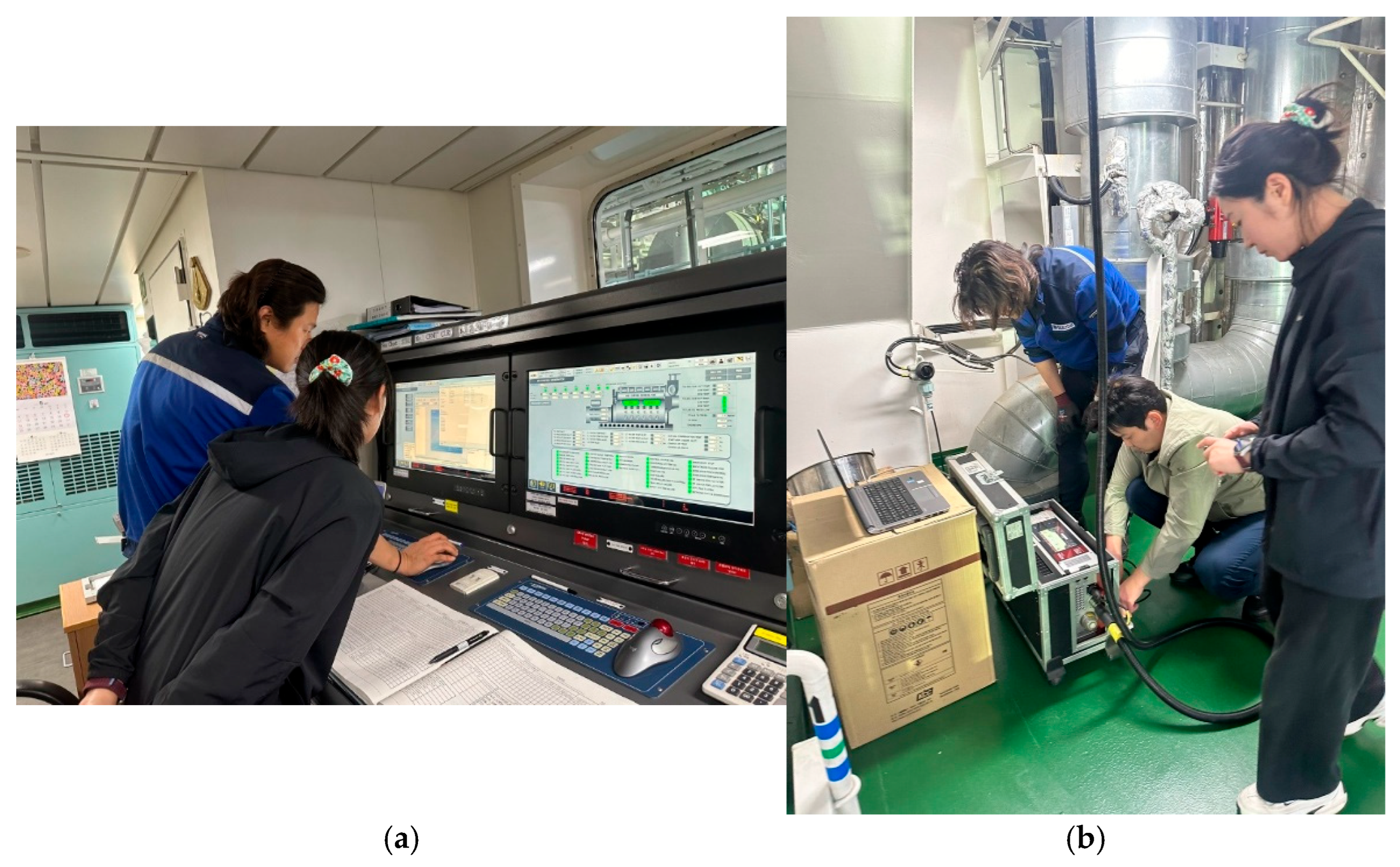
Four data streams were collected onboard the training ship: navigational, meteorological, engine performance, and emissions. Navigational data such as the latitude/longitude, course over ground, and SOG were recorded by a global navigation satellite system (GNSS) receiver and gyrocompass at 1–10 s intervals. Meteorological data were obtained from an ultrasonic anemometer mounted high on the foremast to minimize superstructure interference. The anemometer was calibrated and zero-checked and sampled at ~10 s intervals. Because the anemometer senses the relative wind on the ship frame, the RWS and RWD were used as environmental covariates. The true wind was derived by vector composition with the ship’s velocity vector when required, such as for quality assurance/quality control (QA/QC). Engine performance data were logged at up to 1 Hz and included the engine load (% maximum continuous rating (MCR)), shaft power (kW), engine speed (RPM), CPP pitch (%), and specific fuel oil consumption (SFOC, g/kWh). The SFOC was computed as the ratio of the engine’s instantaneous fuel-mass flow rate to the corresponding shaft power output (g kWh−1). It was therefore based solely on the engine’s mechanical power rather than the combined aerodynamic effects of wind. The aerodynamic influence of the relative wind was analyzed independently through the parameters RWS and RWD. For reference, the main engine of the training ship exhibits a characteristic parabolic SFOC–load relationship with a minimum SFOC occurring at approximately 70–90% of the rated load. Operation below 50% load leads to a rapid rise in SFOC owing to reduced combustion efficiency, whereas CPP adjustments enable the engine to maintain near-optimal conditions under varying environmental resistance. This description has been added to clarify how the SFOC changes with engine load and how the CPP contributes to maintaining efficient operation. Emissions data were sampled every 10–15 s in the main-engine uptake by a continuous emission monitoring system (CEMS) using nondispersive infrared (NDIR) and electrochemical analyzers and included NOx (ppm), SO2 (ppm), and CO2 (% or ppm). Emissions were reported on a dry basis with pre- and post-voyage zero/span checks conducted in accordance with the QA/QC requirements of MARPOL Annex VI Tier III. The extraction of raw data is illustrated in Appendix A (Figure A1 and Figure A2). The analyzer ranges, response times (T90), O2-correction basis, and QA/QC protocols are summarized in Appendix A (Table A1). All data streams were time-stamped with the shipboard clock and later converted to Coordinated Universal Time (UTC) for integration.

2.3. Data Synchronization and Preprocessing

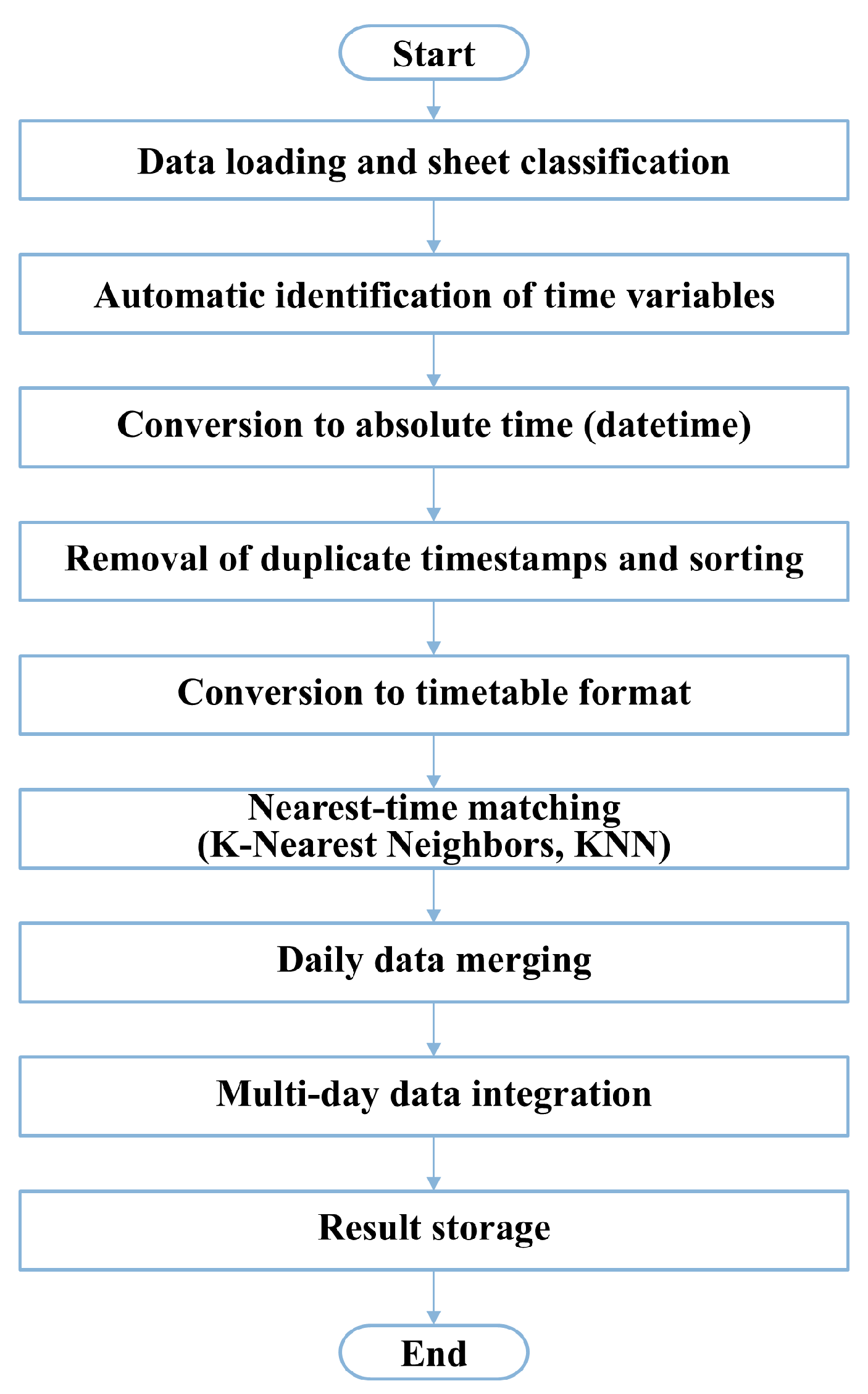
Proper preprocessing of raw data is essential to ensure reliable regression and optimization outcomes. Figure 2 illustrates the data synchronization and preprocessing workflow used in the present study. Raw data were stored in two groups: navigational/meteorological and engine performance/emissions. The two groups of data had different sampling intervals and local time stamps (HH:mm:ss), which made direct integration infeasible. Therefore, calendar dates were appended to convert the data to UTC. Then, duplicates were removed, and the data were sorted chronologically. Finally, data streams were aligned on a common time axis [13,15]. The data were parsed and classified as navigational, meteorological, engine performance, and emissions based on the metadata and column names. Each stream was converted to a timetable and as-of joined (nearest-time match) within ±5 s to align the navigational/meteorological group with the engine performance/emissions group. The unified series was then resampled to a fixed 10 s grid by using median aggregation to reduce noise while preserving dynamics.
To ensure statistical reproducibility and transparency, outliers were detected and removed using two complementary approaches: (1) the Z-score method, where observations with absolute standardized residuals |z| > 3 were excluded, and (2) the interquartile range (IQR) rule, in which values outside [Q1 − 1.5 × IQR, Q3 + 1.5 × IQR] were flagged as outliers. These filters were applied independently to each continuous variable (e.g., engine load, SFOC, NOx, SO2, CO2) to suppress the influence of transient sensor spikes or logging noise. The QA/QC process included the removal of outliers (|z| > 3), removal of segments with continuous missing data (>60 s), and cross-checks among redundant indicators (e.g., SOG versus shaft power). Daily merges were subsequently concatenated across the four voyages, which yielded a consolidated matrix suitable for multivariate analysis and regression modeling that was reduced from 129,632 × 42 data points to 18,178 × 42 data points. Similar challenges in data integration and noise removal have been reported in large-scale studies using automatic identification system (AIS) and engine logs [23].

2.4. Data Analysis and Modeling

The synchronized dataset (18,178 × 42 data points) was used to investigate the influence of relative wind on propulsion efficiency and emissions. The data analysis was designed to quantify correlations, identify statistically significant predictors, and develop operational optimization strategies in compliance with Tier III requirements [1].

2.4.1. Variable Selection

The selected predictor variables included the RWS (kn), RWD (°), engine load (% MCR), engine speed (RPM), and shaft power (kW). The response variables included the NOx concentration (ppm), SO2 concentration (ppm), CO2 concentration (ppm), and SFOC (g/kWh). The RWS and RWD were used instead of their true wind counterparts because they directly reflect the hydrodynamic and aerodynamic forces acting on the hull and propeller and thus provide a more realistic representation of operational conditions [21,22].
The inclusion of both engine load and shaft power was not intended to represent completely independent physical quantities. Indeed, the engine load (expressed as a percentage of the rated power) is directly related to the shaft power delivered to the propeller through the equality of torque, rotational speed, and transmitted power, except for minor transmission losses. However, in full-scale operational conditions, small deviations can occur owing to control settings such as the CPP pitch, transient engine responses, and shafting efficiency variations. Therefore, both variables were retained in the regression model to capture these practically relevant differences and to distinguish between control-side settings (engine load) and output-side responses (measured shaft power). To evaluate potential multicollinearity among predictors, Variance Inflation Factors (VIFs) were calculated for all explanatory variables. All VIF values ranged between 1.2 and 2.8, indicating the absence of severe multicollinearity and confirming that the selected variables contribute independent explanatory power to the regression models.

2.4.2. Data Transformation

To account for the periodic nature of wind direction data (0–360°), the following trigonometric transformation was applied to the RWD:
R W D x = cos ( θ R W D )   and   R W D y = sin ( θ R W D )
This transformation eliminated discontinuity artifacts when the RWD wrapped around 0° and 360° and facilitated linear regression modeling [10,24]. All continuous variables were normalized to a zero mean and unit variance prior to regression to prevent scale dominance in multivariate analysis [19].

2.4.3. Correlation Analysis

Pearson’s correlation coefficient (r) was calculated for each pair of predictor and response variables to identify significant linear relationships. Circular–linear correlation methods were applied for angular variables [24]. The statistical significance threshold was set at p < 0.05 following standard practice in maritime performance studies [15]. Multiple testing corrections were not applied as the analysis was primarily exploratory.

2.4.4. Regression Modeling

Multiple linear regression (MLR) was applied to quantify the combined effects of relative wind conditions and engine parameters on the pollutant emissions and SFOC:
y = β o + i = 1 n β i X i + ϵ
where y represents the response variable (e.g., NOx), Xi represents the predictor variables, and ϵ represents the residual error term. The model performance was evaluated by using the coefficient of determination (R2) and root mean square error (RMSE).
A generalized additive model (GAM) was employed to capture potential nonlinear relationships between the relative wind conditions and emissions [25,26]. While various machine learning approaches such as the artificial neural network, support vector machine, and random forest have been widely applied to predicting the SFOC [27,28,29], they often lack interpretability which is essential for operational decision-making. In contrast, GAM provides a balance between predictive performance and transparency and thus was selected as a representative nonlinear method owing to its interpretability compared with black-box machine learning models [25]. All data preprocessing, statistical analysis, and modeling were conducted using MATLAB R2022b (MathWorks, Natick, MA, USA).

2.4.5. Operational Optimization

The optimization involved determining operational windows that minimize pollutant emissions while maintaining propulsion efficiency [30,31]. The weighted sum approach was used to formulate an objective function that combines the normalized NOx, SO2, and CO2 emissions with the SFOC, which explicitly represents the propulsion efficiency. However, because SO2 and CO2 were found to vary almost proportionally with SFOC and contributed less than 5% to the total variance, only NOₓ and SFOC were explicitly retained in the simplified equation for clarity of presentation. The full weighted objective function was nevertheless computed using all four variables to preserve consistency between the model and the text.
J = ω 1 · N O x N O x , m a x + ω 2 · S F O C S F O C m a x
where ω_1 and ω_2 were determined by prioritizing compliance with Tier III limits over propulsion efficiency (baseline: ω1 > ω2). In addition, an ε-constraint variant (e.g., NOx ≤ ε) was solved to minimize the SFOC. Although full-scale application of advanced multi-objective evolutionary algorithms (e.g., NSGA-II) was beyond the scope of the pre-sent study, a sensitivity analysis with alternative weights was also conducted to assess the robustness of the optimization outcomes [7,8].

2.4.6. Validation

A four-fold voyage-blocked cross-validation procedure was applied to assess the generalization of the regression models and optimization outcomes. The k-fold cross-validation approach is considered robust for modeling the SFOC across diverse voyages [29]. Each fold corresponded to one voyage; the model was trained on data from three voyages and validated on the remaining one. This rotation was repeated four times so that each voyage served once as the validation set. The average predictive performance of the GAM was R2 = 0.98 ± 0.01 and RMSE = 30 ± 4 ppm for NOx emissions, demonstrating strong generalization and low voyage-to-voyage variance. Residual diagnostics confirmed no systematic bias or autocorrelation (Durbin–Watson ≈ 2.0).

3. Results

3.1. Distribution of Relative Wind Conditions and Navigational Characteristics

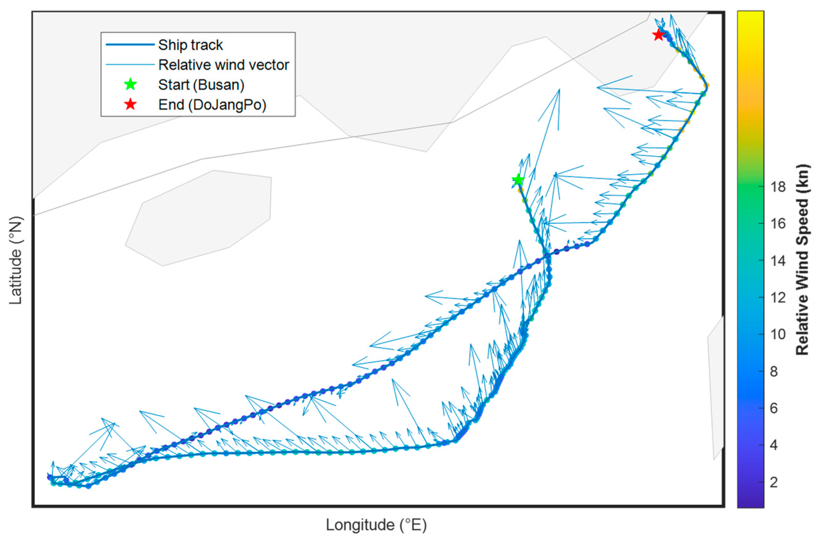
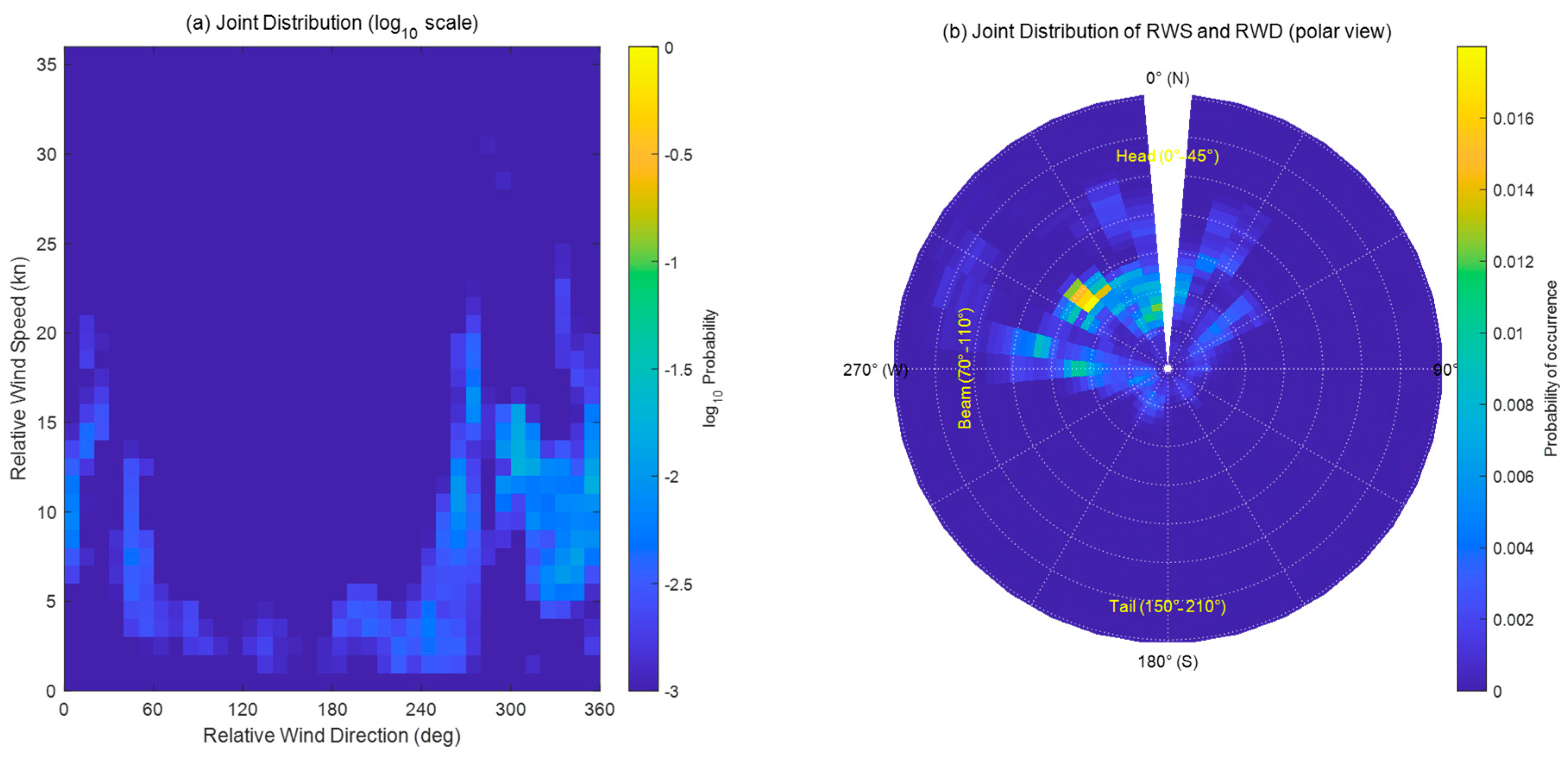
The voyages were strongly influenced by the seasonal monsoon winds, which resulted in diverse relative wind conditions. Approximately 42% of the dataset correspond-ed to headwind conditions (0° ± 45°), 28% corresponded to beam wind conditions (70–110°), and 20% corresponded to tailwind conditions (150–210°). The remaining ~10% of observations corresponded to transitional or oblique wind sectors (approximately 45–70° and 110–150°) that occurred during course changes or maneuvering periods. These records were not classified into a specific sector because the relative wind vectors were highly unstable and short-lived, and their influence on propulsion performance could not be quantified with statistical confidence. The RWS had a range of 2–18 kn with a median of 8.7 kn, which reflects differences engine load caused by aero-dynamic drag. Headwinds increased the pressure drag on the bow, which amplified the hull resistance and increased the engine load for the ship to maintain a constant speed [21,22]. Tailwinds reduced the hull resistance, which lowered the engine load and SFOC. Beam winds exhibited intermediate characteristics because of lateral drag forces. Thus, the relative wind was not a secondary variable but a key determinant of the SFOC and pollutant emissions. As shown in Figure 3, headwinds were stronger during the northbound leg of the voyages, which was attributed to the influence of the seasonal wind patterns. Meanwhile, Figure 4 shows the dominance of the headwind and beam wind sectors, which jointly accounted for ~70% of observations. These findings highlight the necessity of considering the effects of the RWD in statistical analysis and modeling.
Figure 3 and Figure 4 illustrate the navigational tracks and the relative wind conditions recorded during the four voyages. In Figure 3, the northbound leg (Busan → DoJangPo) mainly experienced headwinds, while the southbound return leg encountered beam and tailwinds. Figure 4 shows the corresponding distribution of relative wind speed and direction, highlighting the dominance of head and beam winds during the observation period.

3.2. Changes in Propulsion Efficiency

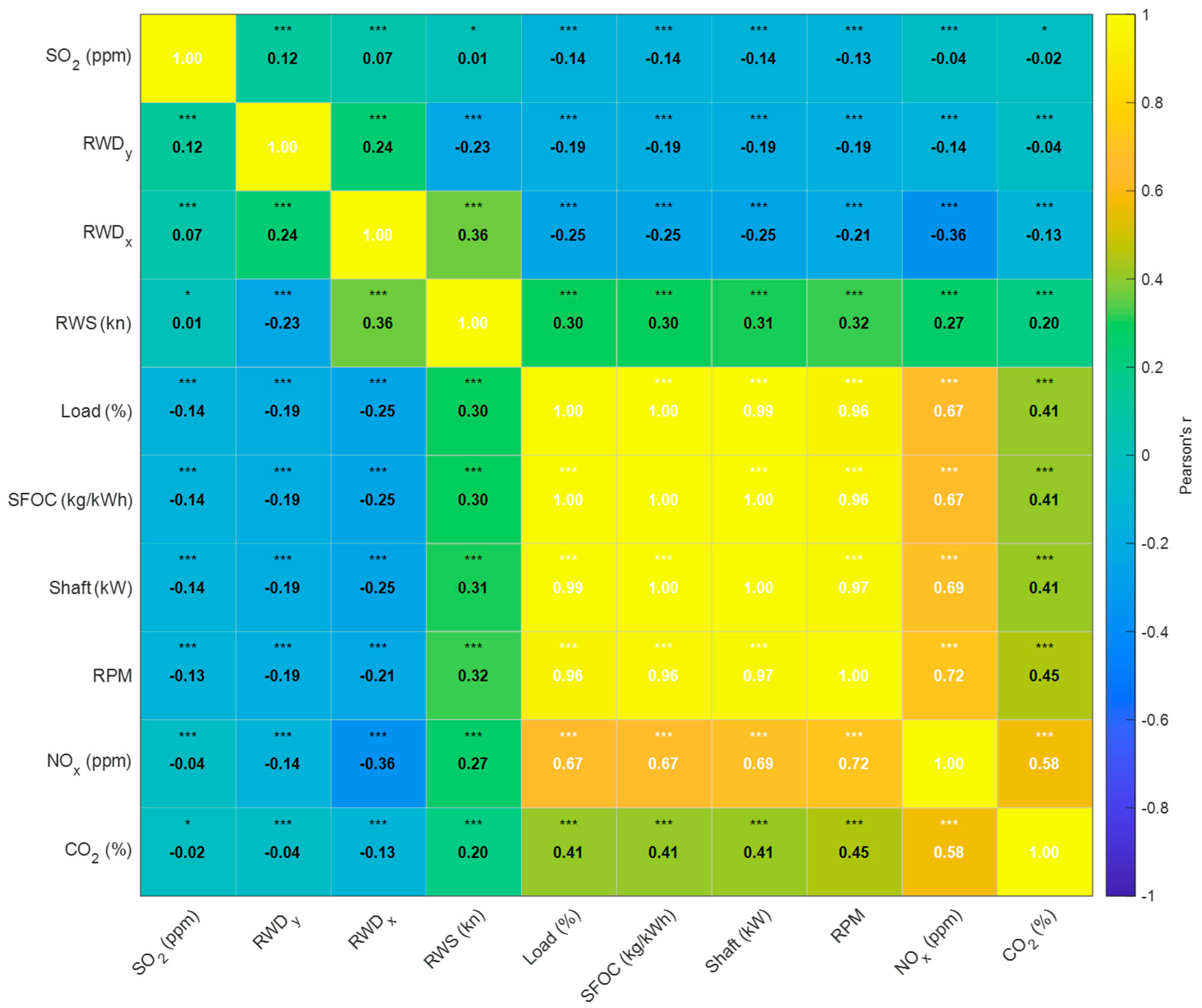
Increasing headwinds increased the hull resistance, which increased the amount of propulsion needed for the training ship to maintain speed. This increased the engine load and shaft power, which resulted in a higher SFOC. Conversely, tailwinds reduced the hull resistance and lowered the SFOC for the same shaft power. These patterns align with fundamental aerodynamic and hydrodynamic principles. Quantitatively, headwinds increased the engine load by ~12% and the SFOC by 8.4 g/kWh. Beam winds increased the engine load by ~6%. Tailwinds reduced the SFOC by up to 6.7 g/kWh. These results confirmed that the relative wind directly affects the propulsion efficiency. The correlation matrix in Figure 5 illustrates the pairwise correlations among the main variables. The relative-wind speed (RWS) showed its strongest linear association with engine speed (RPM) (r = 0.32, p < 0.01), followed by positive correlations with engine load and shaft power. These results indicate that stronger headwinds increase aerodynamic drag, leading to higher engine revolutions and power demand to maintain speed. Conversely, propulsion efficiency (SFOC) is adversely affected under these conditions, confirming the negative impact of headwinds on fuel performance.
In addition to the correlation between predictors and response variables, pairwise correlations among the predictor variables themselves were examined to preliminarily assess potential multicollinearity. All pairwise correlation coefficients were below 0.6, indicating that no single predictor exhibited strong linear dependence on another. This result supports the independence of the selected predictors, consistent with the low VIF values reported in Section 3.4.

3.3. Variations in Emission Characteristics

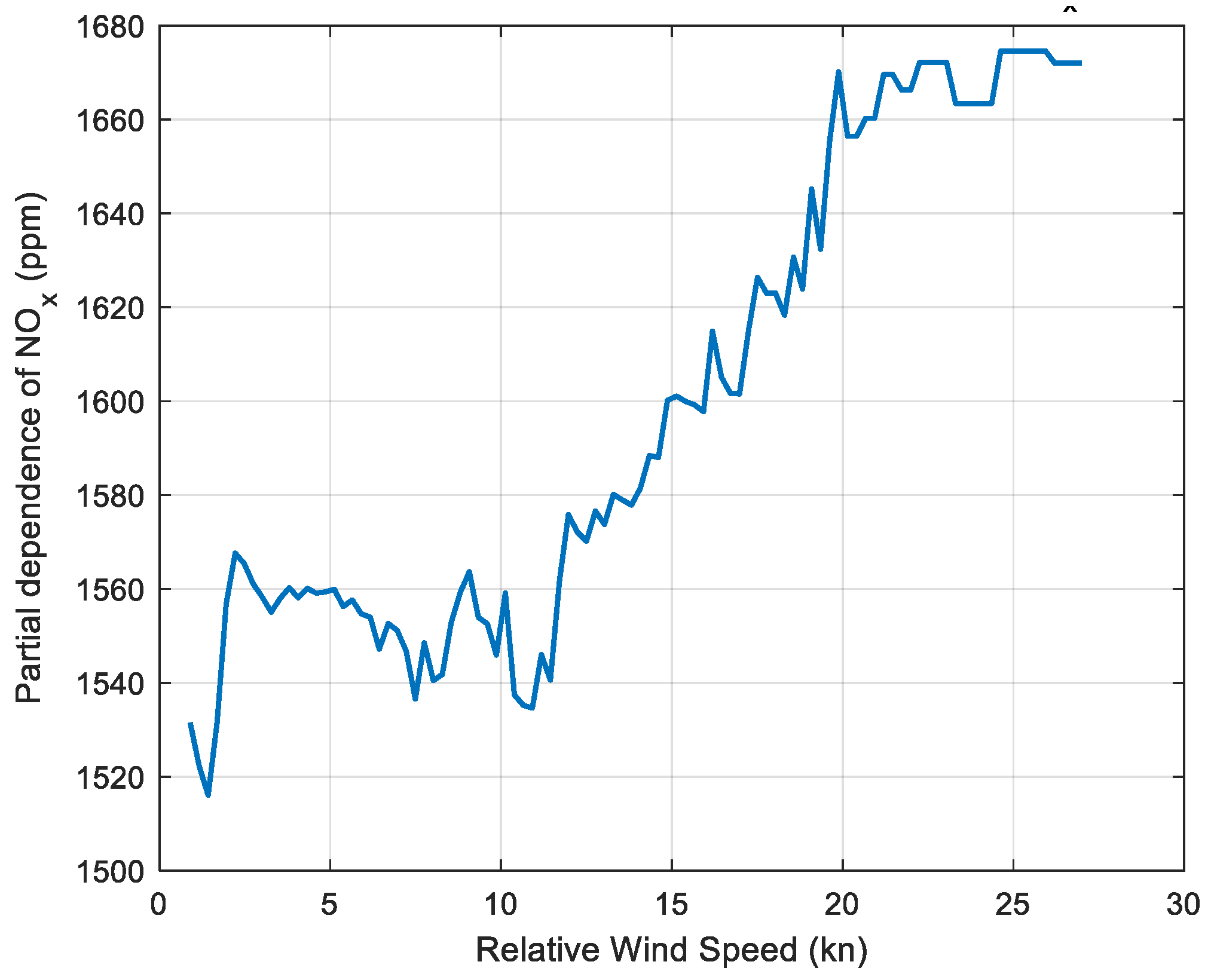
The relative wind conditions also directly influenced pollutant emissions. Headwinds increased the hull resistance and SFOC, which elevated the in-cylinder temperature and pressure and sharply increased NOx emissions. Tailwinds reduced the hull resistance and SFOC, which lowered NOx, SO2, and CO2 emissions. The average NOx concentration was 845 ppm under headwinds, 712 ppm with beam winds, and 655 ppm with tailwinds. Similar patterns were observed for the SO2 and CO2 emissions. In particular, the NOₓ emissions exhibited a nonlinear escalation beyond a relative wind speed (RWS) of approximately 12 kn, reflecting intensified thermal-NOₓ formation at higher combustion temperatures. This threshold was quantitatively derived from the GAM partial-dependence analysis, where the second derivative of the fitted smooth term for RWS changed sign at about 11.8–12.2 kn (p < 0.01). The result confirms that the 12-kn limit is data-driven rather than visually inferred, representing a statistically significant inflection point at which NOₓ emissions begin to rise sharply.

3.4. Regression Modeling

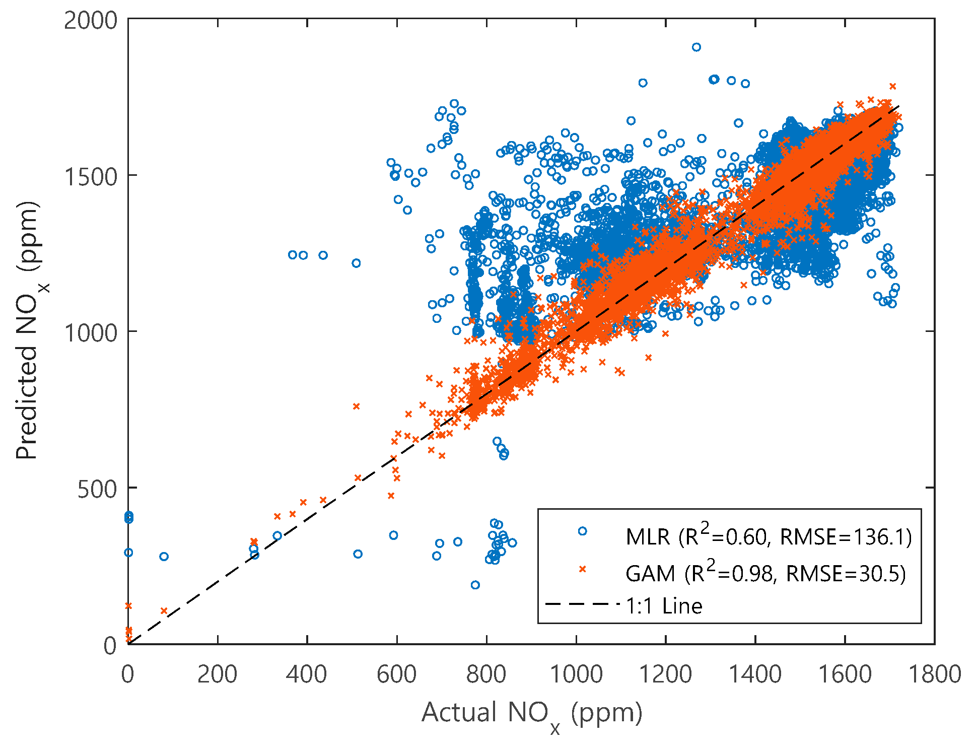
Both MLR and GAM were applied to quantifying interactions between the relative wind conditions and engine parameters. The MLR was used as a baseline linear model to identify first-order linear dependencies and to provide a direct comparison with conventional regression methods widely applied in ship-performance studies. The GAM, on the other hand, extends MLR by incorporating smooth nonlinear functions to capture threshold and interaction effects that cannot be represented by linear models. The comparison between MLR and GAM was therefore designed not as a competition with black-box machine-learning algorithms, but rather to demonstrate the necessity and benefits of nonlinear modeling while maintaining physical interpretability. GAM provides a balance between transparency and predictive accuracy, which is essential for operational decision-making in maritime engineering. Because MLR assumes linearity, it could not capture the nonlinear escalation of pollutant emissions with increasing RWS and thus had a limited explanatory power for NOx emissions (R2 = 0.60, RMSE = 136 ppm).
In contrast, the GAM was configured using thin-plate regression splines as the smoothing basis functions. The smoothing parameters were automatically optimized by generalized cross-validation (GCV) to minimize the prediction error, and the basis dimensions were adaptively determined following the procedure of Wood’s work to avoid over- or under-smoothing [26]. The GAM incorporated two univariate smooth functions for RWS and engine load, as well as a bivariate interaction term that captured their combined nonlinear influence on pollutant emissions and propulsion efficiency. This configuration allowed GAM to represent local nonlinearities and interaction effects, achieving a marked improvement in predictive accuracy (R2 = 0.98, RMSE = 30 ppm). Figure 6 compares the predicted and observed values, confirming the superior fit of GAM. Figure 7 and Figure 8 show that the model effectively captured both the marginal effects of the RWS and its interactions with engine load. The partial-dependence plot in Figure 8 demonstrates a nonlinear amplification of the NOx concentration to greater than 1500 ppm when the engine load exceeded 30% and the RWS exceeded 12 kn. Threshold-like behavior was observed around an RWS of approximately 12 kn, beyond which both NOx emissions and SFOC increased sharply. The sharp rise in SFOC was quantitatively verified from the GAM partial-dependence function of SFOC versus RWS, which showed a statistically significant inflection point at 11.9 ± 0.3 kn (p < 0.01). This confirms that the increase in SFOC beyond 12 kn is data-driven rather than visually interpreted and is consistent with the physical expectation that aerodynamic drag rises disproportionately under strong headwind conditions, leading to higher engine load and fuel consumption. Additionally, VIFs were calculated for all predictor variables, with values ranging between 1.2 and 2.8, confirming that multicollinearity did not influence the regression results. These results were consistent with the pairwise correlation analysis presented in Section 3.2, where all inter-predictor correlation coefficients were below 0.6, further confirming the absence of strong linear dependence among the predictors.
The four-fold voyage-blocked cross-validation confirmed that the GAM maintained high predictive accuracy (R2 = 0.98 ± 0.01, RMSE ≈ 30 ppm) across different voyages, demonstrating its robustness and generalization capability.

3.5. Optimization Results

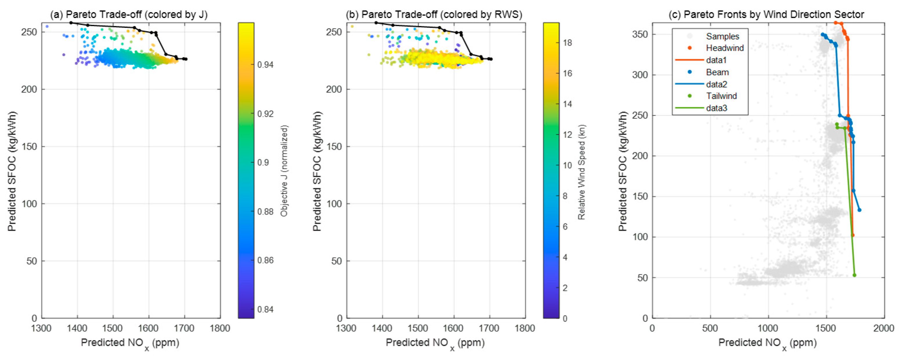
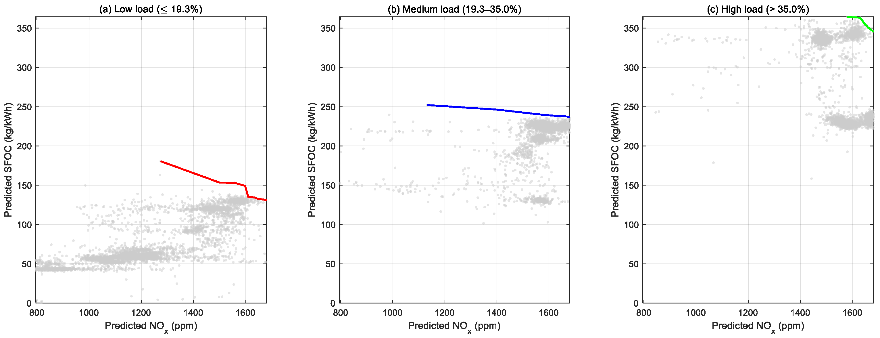
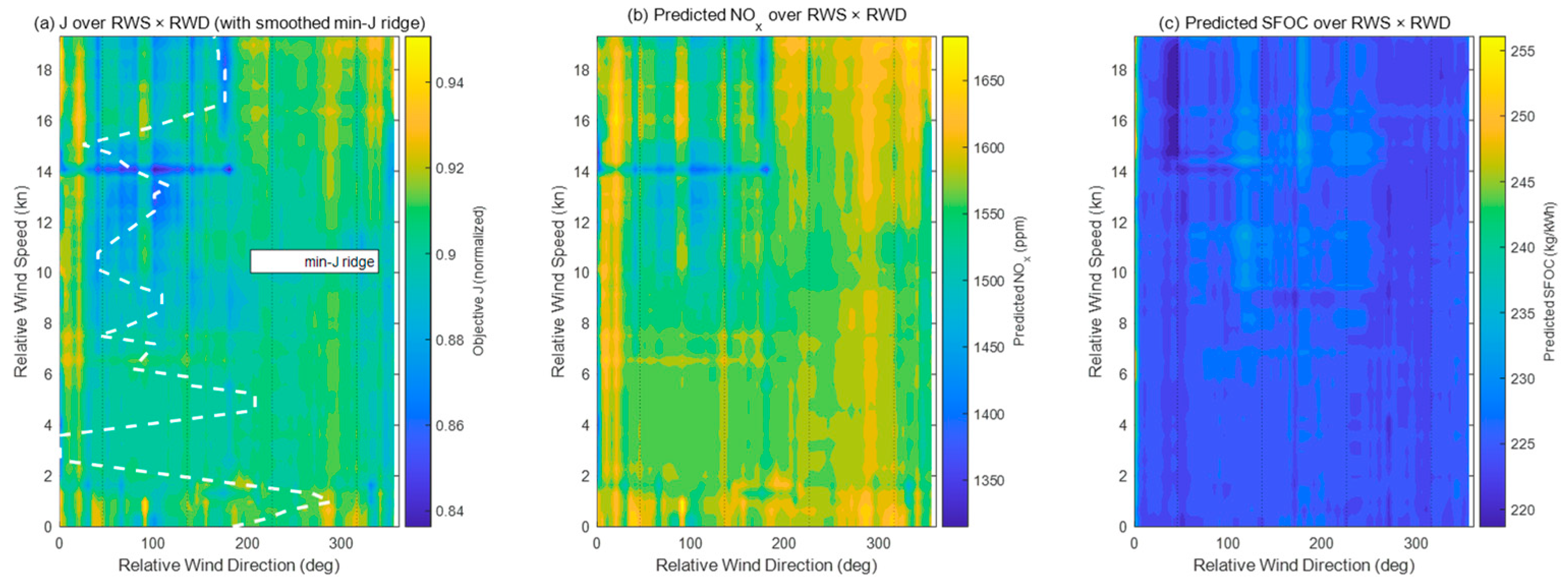
Optimization was conducted using GAM to explore the tradeoff between the SFOC and NOx emissions. The objective function (Equation (3)) was originally formulated to include four response variables—NOx, SO2, CO2, and SFOC—to represent both pollutant control and propulsion efficiency. However, exploratory analysis showed that SO2 and CO2 varied almost proportionally with SFOC, as their formation is directly linked to fuel consumption. As a result, NOx and SFOC emerged as the dominant trade-off pair, while SO2 and CO2 contributed less than 5% to the total variance of the objective function. For clarity of presentation, SO2 and CO2 were retained in the weighted objective formulation but omitted from graphical visualization in Figure 9, Figure 10, Figure 11 and Figure 12. This simplification did not affect the optimization results, as their low variability had a negligible impact on the Pareto fronts. The Pareto fronts varied by wind sector. For headwinds, there was a steep tradeoff between propulsion efficiency and NOx emissions. For beam winds, the Pareto front was more balanced and allowed for moderate compromises. For tailwinds, operational windows were identified where gains in propulsion efficiency and reductions in pollutant emissions could be realized simultaneously. Figure 9 provides predicted Pareto fronts across wind sectors, which show that reducing NOx emissions under headwinds required a steep sacrifice of the SFOC while both the NOx emissions and SFOC could be improved under tailwinds. These results indicate that the relative wind substantially influences the tradeoff between propulsion efficiency and pollutant emissions and that headwinds represent the least favorable conditions. As shown in Figure 10, the observed results and Pareto fronts predicted by GAM agreed closely, which supports the reliability and generalizability of the model. As shown in Figure 11 and Figure 12, two-dimensional mapping analyses incorporating both the RWS and RWD identified an optimal operational window for both improving the propulsion efficiency and reducing NOx emissions: a moderate RWS of 6–10 kn, RWD range of 120–210° encompassing beam winds and tailwinds, and an engine load of 30–40%. The alignment between observed and predicted Pareto fronts was quantitatively confirmed: the root-mean-square deviation between the observed points and the predicted front was <4%, and more than 90% of the observed samples fell within the 95% confidence envelope shown as the shaded region in Figure 9. Figure 10 and Figure 11 visualize the two-dimensional optimization surface predicted by GAM; the ridge of minimum normalized objective function (J) corresponds to the optimal operating window. This ridge region—indicated by darker contours—clearly delineates the RWS range of 6–10 kn and RWD of 120–210° (beam-to-tail winds) at engine-load levels of 30–40%, consistent with the textual conclusions. These results demonstrate that the relative wind is not a passive external factor but an important determinant of the tradeoff between propulsion efficiency and pollutant emissions. Strategically, headwind conditions necessitate a reduction in speed and adjustment of the engine load while beam wind and tailwind conditions provide opportunities for both improving propulsion efficiency and reducing pollutant emissions. Quantitatively, operation within the identified optimal window (RWS 6–10 kn, RWD 120–210°, engine load 30–40%) reduced the average NOₓ emissions by approximately 12% and the SFOC by about 6% compared with the overall voyage mean values. Relative to headwind conditions, these improvements correspond to reductions of nearly 20% in NOx and 10% in SFOC, highlighting the practical significance of adopting wind-aware operational adjustments.

4. Discussion

This study quantitatively assessed the influence of relative wind conditions on the propulsion efficiency and emissions of a training ship using full-scale voyage data. The data analysis revealed that the engine load and SFOC increased under headwinds, which was coupled with a nonlinear surge in NOx emissions. These findings reflect the combined effects of the hydrodynamic response of the hull–propeller system and the thermodynamic behavior of the engine.

4.1. Physical Interpretation

An intensifying headwind increases the pressure drag on the bow, which raises the overall hull resistance. To maintain a constant speed, the shaft power must be increased, which increases the engine load and SFOC. A higher engine load increases the in-cylinder temperature and pressure, which promotes thermal-NOx formation and leads to a sharp rise in pollutant emissions. The observed threshold-like escalation of NOx beyond an RWS of ~12 kn is consistent with combustion theory although additional factors such as wave-induced resistance may also contribute. In contrast, tailwinds reduce the hull resistance and shaft power, which reduces both the SFOC and pollutant emissions. These results indicate that the tradeoff between propulsion efficiency and pollutant emissions is fundamentally shaped by the RWD.

4.2. Comparison with Previous Studies

Previous studies have shown that the wind direction and speed affect the hull resistance [21,22]. However, most relied on numerical simulations or towing-tank experiments and did not incorporate in-service emission characteristics. By linking the relative wind conditions with propulsion efficiency and pollutant emissions using full-scale operational data, this study provides more practical and empirical insights. Furthermore, unlike recent data-driven research focused primarily on predicting the SFOC [16,19], this work integrates external environmental variables such as wind into an optimization framework that explicitly includes pollutant emissions, which extends its applicability. Recent reviews have classified SFOC models into white-box, black-box, and gray-box approaches [32]. White-box models [33,34] rely on resistance formulations but often lack accuracy in operational settings. Black-box models [27,28,35,36] achieve a high predictive accuracy but have been criticized for limited interpretability. Gray-box methods [37] combine physical insights with data-driven fitting. In this context, the GAM can be regarded as a gray-box approach, as it models nonlinear effects of environmental and engine parameters through interpretable smooth functions. This allows identifying the physical influence of wind and propulsion variables while maintaining the flexibility of da-ta-driven learning. Accordingly, this study applied GAM to capture nonlinear effects while maintaining interpretability, thereby addressing a recognized gap between accuracy and transparency in support of operational decision-making.

4.3. Operational Implications

The results offer practical implications for operational decision-making and maritime autonomous surface ship (MASS) control strategies. Under strong headwinds, the propulsion efficiency of a ship decreases while pollutant emissions increase, which makes it necessary to adopt measures such as slow steaming, CPP adjustment, or modified engine settings to suppress escalation of the engine load. In contrast, beam wind and tailwinds allow the propulsion efficiency and pollutant emissions to be improved simultaneously. Incorporating relative wind conditions into voyage planning may facilitate more cost-effective compliance with Tier III limits [6]. Meanwhile, MASS control systems that integrate relative wind conditions as a real-time decision variable could provide more effective management of the propulsion efficiency and pollutant emissions. Similar multi-objective optimization frameworks have been applied in the context of speed and route planning [38]. In the present study, the data analysis based on Pareto fronts illustrated that tradeoffs between the propulsion efficiency and pollutant emissions are strongly dependent on relative wind conditions.

4.4. Limitations and Future Work

The findings of this study are subject to several limitations. First, the dataset was limited to four voyages of a single training ship, which restricts the generalizability of the results across ship types and operational conditions. Second, the effects of waves and currents were not explicitly included, leaving certain variations in hull resistance unexplained. Third, detailed logs on engine performance data, such as the CPP pitch angle and auxiliary loads, were unavailable, limiting finer attribution of engine load changes. Fourth, although the GAM provided a strong fit, the high R2 may partly reflect voyage-specific dynamics. External validation with independent datasets is therefore required. Fifth, while the study discussed the relationships identified through GAM, a more operational perspective can be drawn from the model’s interpretability. Specifically, the partial dependence plots revealed that propulsion efficiency tends to decline sharply when the relative wind speed exceeds approximately 12 knots or when the engine load falls below 60% of rated power. These patterns indicate that maintaining the engine load in the 70–90% range and minimizing prolonged headwind exposure could enhance energy efficiency and reduce emissions, thereby supporting decision-making for voyage planning and power management. Finally, the optimization framework was limited to scalarized formulations. Future work should employ full Pareto-based evolutionary algorithms to capture multidimensional trade-offs. Multivariate data fusion (e.g., wave estimation algorithms under ISO 15016 [13]) and advanced statistical frameworks such as generalized additive mixed models or Bayesian hierarchical models should be incorporated to capture voyage-level random effects. Extending the optimization framework to large-scale AIS–engine log datasets will be essential to validate its robustness across diverse ship types and environments.

5. Conclusions

This study quantitatively demonstrated the influence of relative wind conditions on the propulsion efficiency and pollutant emissions of a training ship using full-scale navigational data. The results indicated that the RWS and RWD are important determinants of the observed tradeoff between propulsion efficiency and pollutant emissions. While the results may not be universally generalizable, they highlight the necessity of considering wind vectors in operational decision-making and future MASS control strategies.
Analysis of the relative wind distributions revealed that headwind and beam wind conditions accounted for about 70% of the voyage data. Under headwinds, the engine load increased by approximately 12% and the SFOC rose by 8.4 g/kWh. Under tailwinds, the SFOC decreased by up to 6.7 g/kWh at the same shaft power. In terms of pollutant emissions, the average NOx concentration was about 845 ppm under headwinds while only 712 ppm under beam winds and 655 ppm under tailwinds. A nonlinear threshold effect was observed where the RWS exceeded 12 kn with NOx emissions surpassing 1500 ppm under combined high-load and high-wind conditions. Regression modeling showed that, while MLR failed to capture nonlinear effects, GAM successfully reflected local threshold behavior to achieve a high explanatory power (R2 = 0.98). This underscores the necessity of nonlinear models to interpret wind–load interactions and their effects on the tradeoff between propulsion efficiency and pollutant emissions. Optimization analysis identified distinct Pareto fronts across wind sectors. Under headwinds, reducing NOx emissions required a substantial sacrifice of propulsion efficiency. In contrast, beam wind and tailwind conditions allowed simultaneous improvement of both the NOx emissions and propulsion efficiency. An optimal operational window was identified for beam winds and tailwinds at a moderate RWS of 6–10 kn and engine load of 30–40%.
The findings provide actionable insights for improving the propulsion efficiency and reducing the pollutant emissions of ships based on actual operational data. In particular, integrating relative wind conditions as real-time decision variables can help MASSs comply with Tier III limits in a cost-effective manner. Future research should involve expanding the optimization framework to incorporate additional environmental factors such as waves and currents as well as the CPP pitch and validating its generalizability across diverse ship types and operating conditions through large-scale integration of AIS and engine log data.

Author Contributions

Conceptualization, S.-A.P. and S.-H.J.; Methodology, S.-A.P.; Software, S.-A.P. and D.-J.P.; Validation, M.-A.J.; Formal analysis, D.-J.P.; Investigation, S.-H.J. and D.-J.P.; Data curation, S.-A.P. and M.-A.J.; Writing – original draft, S.-A.P.; Writing – review & editing, D.-J.P.; Visualization, D.-J.P.; Supervision, D.-J.P.; Project administration, D.-J.P.; Funding acquisition, D.-J.P. All authors have read and agreed to the published version of the manuscript.

Funding

This research was supported by the Regional Innovation System & Education (RISE) program through the Institute for Regional Innovation System & Education in Busan Metropolitan City, funded by the Ministry of Education (MOE) and the Busan Metropolitan City, Republic of Korea. (2025-RISE-02-001-006).

Data Availability Statement

As the raw operational data include sensitive information related to ship operations, the data cannot be made publicly available. However, processed and anonymized data supporting the findings can be provided by the corresponding author upon reasonable request.

Acknowledgments

The authors gratefully acknowledge the captain and crew of the training ship Baekkyung of Pukyong National University for their kind assistance and cooperation during the practical training and onboard data collection.

Conflicts of Interest

The authors declare no conflict of interest.

Appendix A

Figure A1. Extraction of raw engine performance and pollutant emissions data: (a) Engine control room with the interface used to record the engine load (% MCR), engine speed (RPM), shaft power (kW), CPP pitch (%), and SFOC (g/kWh). (b) CEMS sampling at the main-engine uptake (NDIR/electrochemical analyzers) and sample line connection with pre-/post-voyage zero/span checks.
Jmse 13 02120 g0a1
Figure A2. Extraction of raw navigational and meteorological data. (a) Bridge operations with the ultrasonic anemometer for measuring relative wind conditions on the foremast. (b) ECDIS display used to export GNSS track and hydrographic context for deriving COG, SOG, and relative wind vectors.
Jmse 13 02120 g0a2
Table A1. Analyzer ranges, response times (T90), O2-correction basis, and QA/QC protocols.
Measuring RangeResponse Time T90
O20–25 Vol%<20 s
CO0–10,000 ppm<40 s
NO0–1000 ppm<30 s
NO20–200 ppm<40 s
SO20–2000 ppm<40 s
C r e f = C m e a s · 21 O 2 , r e f 21 O 2 , m e a s
CrefConcentration corrected to reference O2 content (ppm or mg/m3)
CmeasMeasured concentration (ppm or mg/m3)
O2,refReference O2 content (typically 13% for marine diesel engines)
O2,measMeasured O2 content in exhaust gas (%)
21O2 content in dry ambient air (%)
All measured emission concentrations were normalized to 13% O2 to enable consistent comparison across different engine loads and fuel conditions.

References

  1. Olaniyi, E.O.; Solarte-Vasquez, M.C.; Inkinen, T. Smart Regulations in Maritime Governance: Efficacy, Gaps, and Stakeholder Perspectives. Mar. Pollut. Bull. 2024, 202, 116341. [Google Scholar] [CrossRef]
  2. International Maritime Organization (IMO). Resolution MEPC.328(76): 2021 Revised MARPOL Annex VI (EEXI/CII, etc.); IMO: London, UK, 2021. [Google Scholar]
  3. Comer, B.; Sathiamoorthy, B. How Updating IMO Regulations Can Promote Lower Greenhouse Gas Emissions from Ships; International Council on Clean Transportation: Washington, DC, USA, 2022. [Google Scholar]
  4. Hurren, T. NOx Measurement and Characterization in a Gaseous Fueled High-Pressure Direct-Injection Engine. Ph.D. Thesis, University of British Columbia, Vancouver, BC, Canada, 2022. [Google Scholar]
  5. Zhu, Y.; Li, Q.; Zhang, M.; Li, H. Application and Development of Selective Catalytic Reduction Technology for Marine Low-Speed Diesel Engines: Trade-Off among High-Sulfur Fuel, High Thermal Efficiency, and Low Pollution Emission. Atmosphere 2022, 13, 731. [Google Scholar] [CrossRef]
  6. Farkas, A.; Degiuli, N.; Martić, I.; Mikulić, A. Benefits of slow steaming in realistic sailing conditions along different sailing routes. Ocean Eng. 2023, 275, 114143. [Google Scholar] [CrossRef]
  7. Çetin, O.; Sogut, M.Z. A new strategic approach of energy management onboard ships supported by exergy and economic criteria: A case study of a cargo ship. Ocean Eng. 2021, 219, 108137. [Google Scholar] [CrossRef]
  8. Hüffmeier, J.; Johanson, M. State-of-the-art methods to improve energy efficiency of ships. J. Mar. Sci. Eng. 2021, 9, 447. [Google Scholar] [CrossRef]
  9. Wang, A.; Liu, Y.; Meng, B.; Lv, H. Tracing the CO2 emissions embodied in Chinese mainland’s exports with multinational enterprises: From source to sink. J. Clean. Prod. 2023, 414, 137430. [Google Scholar] [CrossRef]
  10. Grlj, C.G.; Degiuli, N.; Tuković, Ž.; Farkas, A.; Martić, I. The effect of loading conditions and ship speed on the wind and air resistance of a containership. Ocean Eng. 2023, 273, 113991. [Google Scholar] [CrossRef]
  11. Tran, N.K.; Lam, J.S.L. Effects of container ship speed on CO2 emission, cargo lead time and supply chain costs. Res. Transp. Bus. Manag. 2022, 43, 100723. [Google Scholar] [CrossRef]
  12. Chen, Z.S.; Lam, J.S.L.; Xiao, Z. Prediction of Harbour Vessel Emissions Based on Machine Learning Approach. Transp. Res. Part D Transp. Environ. 2024, 131, 104214. [Google Scholar] [CrossRef]
  13. ISO 15016:2015; Guidelines for the Assessment of Speed and Power Performance by Analysis of Speed Trial Data. International Organization for Standardization: Geneva, Switzerland, 2015.
  14. Park, H.; Lee, P.; Kim, J.; Kim, H.; Lee, H.; Lee, Y. Study on the Estimation Method of Wind Resistance Considering Self-Induced Wind by Ship Advance Speed. J. Mar. Sci. Eng. 2024, 12, 1694. [Google Scholar] [CrossRef]
  15. La Ferlita, A.; Qi, Y.; Di Nardo, E.; El Moctar, O.; Schellin, T.E.; Ciaramella, A. A Framework of a Data-Driven Model for Ship Performance. Ocean Eng. 2024, 309, 118486. [Google Scholar] [CrossRef]
  16. Lee, J.; Eom, J.; Park, J.; Jo, J.; Kim, S. The Development of a Machine Learning-Based Carbon Emission Prediction Method for a Multi-Fuel-Propelled Smart Ship by Using Onboard Measurement Data. Sustainability 2024, 16, 2381. [Google Scholar] [CrossRef]
  17. Ning, Y.; Liu, X.; Sun, P.; Zhang, X.; Gao, Y. Data-driven regional ship carbon emissions using AIS. Sustainability 2025, 17, 1159. [Google Scholar] [CrossRef]
  18. Berghout, T.; Mouss, L.H.; Bentrcia, T.; Elbouchikhi, E.; Benbouzid, M. A deep supervised learning approach for condition-based maintenance of naval propulsion systems. Ocean Eng. 2021, 221, 108525. [Google Scholar] [CrossRef]
  19. Nguyen, V.G.; Sakthivel, R.; Rudzik, K.; Kozak, J.; Sharma, P.; Pham, N.D.K.; Nguyen, X.P. Using Artificial Neural Networks for Predicting Ship Fuel Consumption. Pol. Marit. Res. 2023, 30, 3–13. [Google Scholar] [CrossRef]
  20. Byun, H.R.; Lee, D.K. Defining Three Rainy Seasons and the Hydrological Summer Monsoon in Korea Using Available Water Resources Index. J. Meteorol. Soc. Jpn. Ser. II 2002, 80, 33–44. [Google Scholar] [CrossRef]
  21. Isherwood, R.M. Wind resistance of merchant ships. Trans. R. Inst. Nav. Archit. 1973, 115, 327–338. [Google Scholar]
  22. Blendermann, W. Parameter identification of wind loads on ships. J. Wind. Eng. Ind. Aerodyn. 1994, 51, 339–351. [Google Scholar] [CrossRef]
  23. Emmens, T.; Amrit, C.; Abdi, A.; Ghosh, M. The Promises and Perils of Automatic Identification System Data. Expert Syst. Appl. 2021, 178, 114975. [Google Scholar] [CrossRef]
  24. Berens, P. CircStat: A MATLAB toolbox for circular statistics. J. Stat. Softw. 2009, 31, 1–21. [Google Scholar] [CrossRef]
  25. Hastie, T.J.; Tibshirani, R.J. Generalized Additive Models; Routledge: London, UK, 1990; pp. 136–173. [Google Scholar] [CrossRef]
  26. Wood, S.N. Generalized Additive Models: An Introduction with R, 2nd ed.; Chapman & Hall/CRC: Boca Raton, FL, USA, 2017. [Google Scholar] [CrossRef]
  27. Uyanik, T.; Arslanoglu, Y.; Kalenderli, O. Ship Fuel Consumption Prediction with Machine Learning. In Proceedings of the 4th International Mediterranean Science and Engineering Congress, Antalya, Turkey, 25–27 April 2019. [Google Scholar]
  28. Gkerekos, G.; Lazakis, I.; Theotokatos, G. Ship fuel consumption prediction using machine learning methods. Ocean Eng. 2019, 188, 106282. [Google Scholar] [CrossRef]
  29. Hu, Z.; Jin, Y.; Hu, Q.; Sen, S.; Zhou, T.; Osman, M.T. Prediction of fuel consumption for enroute ship based on machine learning. IEEE Access 2019, 7, 119497–119505. [Google Scholar] [CrossRef]
  30. Deb, K. Multi-Objective Optimisation Using Evolutionary Algorithms: An Introduction. In Multi-Objective Evolutionary Optimisation for Product Design and Manufacturing; Wang, L., Ng, A.H.C., Deb, K., Eds.; Springer: London, UK, 2011; pp. 3–34. [Google Scholar]
  31. La Ferlita, A.; Qi, Y.; Di Nardo, E.; El Moctar, O.; Schellin, T.E.; Ciaramella, A. A comparative study to estimate fuel consumption: A simplified physical approach against a data-driven model. J. Mar. Sci. Eng. 2023, 11, 850. [Google Scholar] [CrossRef]
  32. Leifsson, L.Þ.; Sævarsdóttir, H.; Sigurðsson, S.Þ.; Vésteinsson, A. Grey-box modeling of an ocean vessel for operational optimization. Simul. Model. Pract. Theory 2008, 16, 923–932. [Google Scholar] [CrossRef]
  33. Tillig, F.; Ringsberg, J.W. A 4 DOF simulation model developed for fuel consumption prediction of ships at sea. Ships Offshore Struc. 2019, 14 (Suppl. S1), 112–120. [Google Scholar] [CrossRef]
  34. Guo, B.; Liang, Q.; Tvete, H.A.; Brinks, H.; Vanem, E. Combined machine learning and physics-based models for estimating fuel consumption of cargo ships. Ocean Eng. 2022, 255, 111435. [Google Scholar] [CrossRef]
  35. Wang, S.; Ji, B.; Zhao, J.; Liu, W.; Xu, T. Predicting ship fuel consumption based on LASSO regression. Transp. Res. D Trans. Environ. 2018, 65, 817–824. [Google Scholar] [CrossRef]
  36. Szlapczynska, J.; Szlapczynski, R. Preference-based evolutionary multi-objective optimization in ship weather routing. Appl. Soft Comput. 2019, 84, 105742. [Google Scholar] [CrossRef]
  37. Yang, L.; Chen, G.; Rytter, N.G.M.; Zhao, J.; Yang, D. A genetic algorithm-based grey-box model for ship fuel consumption prediction towards sustainable shipping. Ann. Oper. Res. 2025, 349, 525–551. [Google Scholar] [CrossRef]
  38. Lashgari, M.; Akbari, A.A.; Nasersarraf, S. A new model for simultaneously optimizing ship route, sailing speed, and fuel consumption in a shipping problem under different price scenarios. Appl. Ocean Res. 2021, 113, 102725. [Google Scholar] [CrossRef]
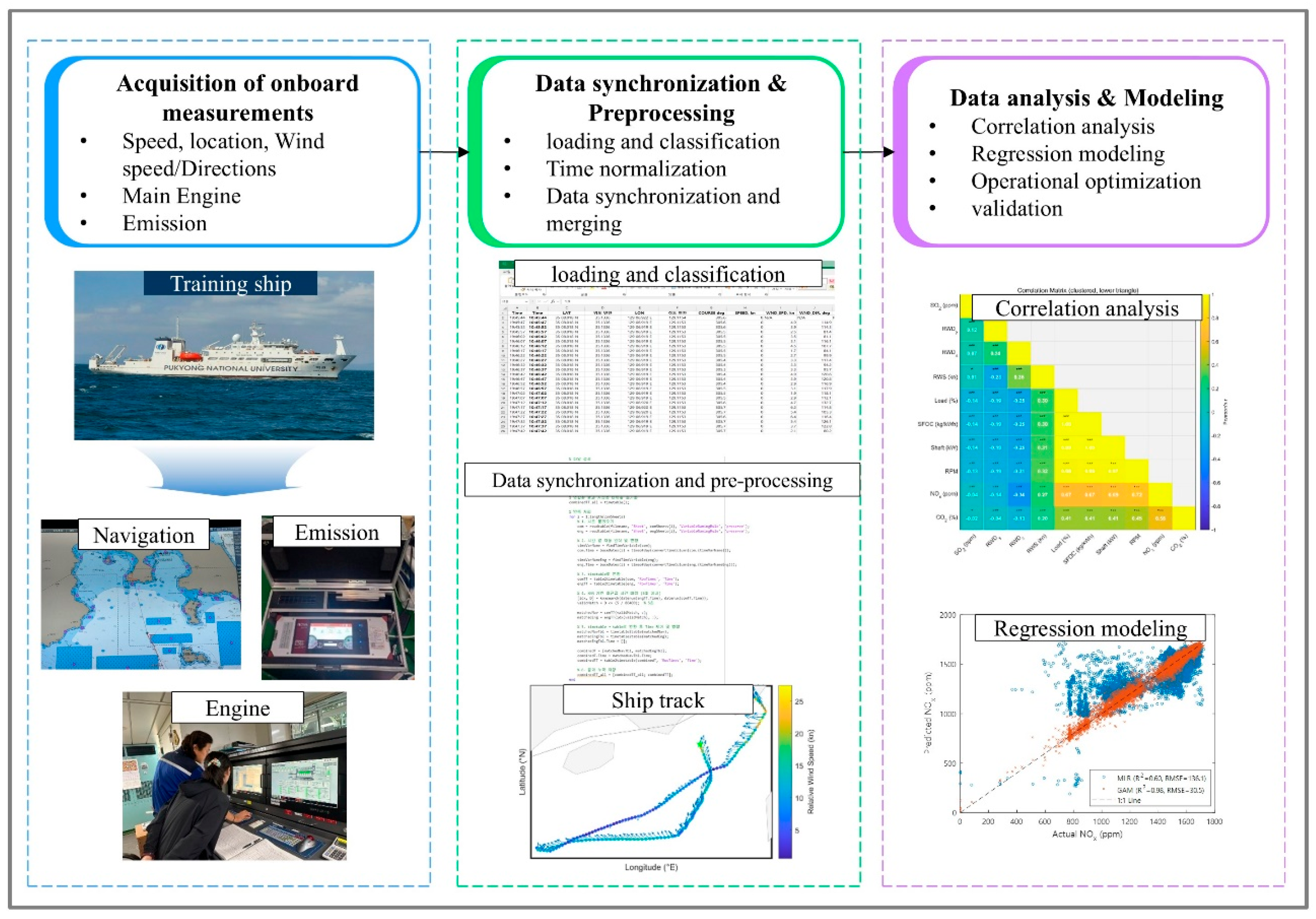
Figure 1. Workflow of the study: onboard data acquisition, data synchronization and preprocessing, and data analysis and modeling.
Jmse 13 02120 g001
Figure 2. Data synchronization and preprocessing workflow.
Jmse 13 02120 g002
Figure 3. Navigational track of the training ship during the voyages. The RWD is indicated by arrows while the RWS is color coded.
Jmse 13 02120 g003
Figure 4. Distribution of relative wind conditions during the voyages. (a) Joint probability density of relative wind speed (RWS) and direction (RWD) shown on a log10 scale. (b) Polar plot of the same dataset illustrating the relative frequencies of head (0–45°), beam (70–110°), and tail (150–210°) wind sectors. R represents wind-speed magnitude (kn) and θ the relative-wind direction (deg). Colors correspond to the probability of occurrence.
Jmse 13 02120 g004
Figure 5. Correlation matrix of predictor and response variables. Each cell displays the Pearson correlation coefficient (r). Positive values indicate direct relationships (e.g., RWS with RPM and engine load), whereas negative values reflect adverse effects on propulsion efficiency (SFOC) under strong headwinds. Color intensity corresponds to the magnitude of correlation. * p < 0.05; *** p < 0.01.
Jmse 13 02120 g005
Figure 6. Predicted NOx emission with multiple linear regression (MLR) and generalized additive models (GAM).
Jmse 13 02120 g006
Figure 7. Partial dependence of NOx emission on relative wind speed (RWS) predicted with GAM.
Jmse 13 02120 g007
Figure 8. Two-dimensional partial dependence of NOₓ emissions on the relative wind speed (RWS) and engine load.
Jmse 13 02120 g008
Figure 9. Pareto fronts predicted by GAM for SFOC and NOₓ emissions across wind sectors: (a) headwinds, (b) beam winds, and (c) tailwinds. Colored dots indicate the predicted samples, and the black lines and circles denote the GAM-predicted Pareto fronts and optimal points, respectively. Headwinds show a steep trade-off, while tailwinds allow the propulsion efficiency to be improved and pollutant emissions to be reduced simultaneously.
Jmse 13 02120 g009
Figure 10. Comparison of observed data with Pareto fronts predicted by GAM for the SFOC and NOx emissions across wind sectors: (a) headwinds, (b) beam winds, and (c) tailwinds. Dots represent observations; solid lines (blue, green, and orange) indicate the GAM-predicted Pareto fronts for each wind sector; shaded bands denote the 95% confidence intervals. More than 90% of the observations lie within this interval, confirming the model’s predictive consistency.
Jmse 13 02120 g010
Figure 11. Predicted SFOC and NOx emissions at (a) low, (b) medium, and (c) high engine loads. Colored lines (red, blue, and green) represent the GAM-predicted Pareto fronts corresponding to different engine-load conditions. Darker contours indicate lower normalized objective function values.
Jmse 13 02120 g011
Figure 12. RWD–RWS maps: (a) normalized objective function J with identified min-J ridge, (b) predicted NOx emissions, and (c) predicted SFOC. The dark ridge of minimum J (white dotted line) represents the optimal operating window (6–10 kn RWS, 120–210° RWD, 30–40% engine load), and the dotted line in (a) indicates the boundary of the low-J region predicted by the model.
Jmse 13 02120 g012
Table 1. Specifications of the training ship Baekkyung.
ParameterValue
Length Overall (LOA)97.0 m
Length Between Perpendiculars (LBP)85.0 m
Breadth15.4 m
Gross tonnage3997 t
Maximum speed16.0 kn
Service speed15.2 kn
Main engine typeTwo-stroke low-speed diesel
Main engine output4727 PS × 167 rpm
PropellerFour-blade CPP
Disclaimer/Publisher’s Note: The statements, opinions and data contained in all publications are solely those of the individual author(s) and contributor(s) and not of MDPI and/or the editor(s). MDPI and/or the editor(s) disclaim responsibility for any injury to people or property resulting from any ideas, methods, instructions or products referred to in the content.