Autonomous Navigation Control and Collision Avoidance Decision-Making of an Under-Actuated ASV Based on Deep Reinforcement Learning

Abstract

For efficient and safe navigation for an autonomous surface vehicle (ASV), this paper proposes an autonomous navigation behavior framework that integrates deep reinforcement learning (DRL) to achieve autonomous decision-making and low-level control actions in path following and collision avoidance. By controlling both the propeller speed and the rudder angle, the policy of each behavior pattern is trained with the soft actor–critic (SAC) algorithm. Moreover, a dynamic obstacle trajectory predictor based on the Kalman filter and the long short-term memory module is developed for obstacle avoidance. Simulations and physical experiments using an under-actuated very large crude carrier (VLCC) model indicate that our DRL-based method produces appreciable performance gains in ASV autonomous navigation under environmental disturbances, which enables forecasting of the expected state of a vessel over a future time and improves the operational efficiency of the navigation process.

1. Introduction

The advancement of maritime transportation highlights the significance of ship decision-making and control methods, which are vital for maintaining the safety and efficiency of ship navigation [1]. While human factors are critical for traditional ship navigation, they are the leading causes of maritime accidents [2]. Autonomous surface vehicles (ASVs) have the potential to minimize human error, thereby guaranteeing more secure operations [3]. When an ASV sails in open water, and its route is pre-determined, it primarily depends on the path-following control approach to ensure reliable navigation, whereas in complicated environments like ports or island regions, it is necessary for the ASV to automatically detect and avoid obstacles with local information. The conventional ASV lacks sufficient control inputs for managing motions in six-degrees of freedom (DOF), which categorizes them as under-actuated systems. External factors like wind, wave, and current can greatly impact the motion control. Therefore, it is essential for the ASV to possess real-time and robust path-following control and collision avoidance decision-making functions to minimize the path tracking deviations, resist external disturbances, and improve operational efficiency during navigation.

In recent years, artificial intelligence technology, especially reinforcement learning (RL), has garnered widespread attention for its potential in handling complex decision-making and control challenges. The goal of RL is to learn an optimal policy by facilitating interactions between the agent and the environment. It demonstrates application prospects in fields like autonomous driving and drone flight [4,5]. Although RL has made considerable progress in various domains, its utilization in the navigation of ASVs still remains at an early stage. Marine vehicles are required to analyze various environmental data in real time and adapt to ever-changing obstacles and complex sea conditions. Traditional rule-based methods [6,7,8] have the weakness of poor scalability and tend to be inflexible when dealing with dynamic marine settings. Additionally, model-based control and decision-making approaches [9,10,11] often depend on a precise ship mathematical model. In comparison, RL or deep reinforcement learning (DRL) algorithms transform inputs from multiple channels into executable outputs within a black-box framework. An RL-based algorithm eliminates the necessity for manually established rules and exact specifications. Moreover, it is capable of handling features that are not easy to directly quantify, such as images, natural language, etc. [12]. Ref. [13] achieved ship path following through a line-of-sight guidance algorithm and subsequently trained a collision avoidance policy utilizing the proximal policy optimization algorithm. This approach was verified under unknown environmental disturbances. However, the state space incorporated global coordinate information, and the policy need to be retrained in new scenarios. Ref. [14] developed a dual-layer navigation system comprising a long-term planner and a short-term decision maker using a deep Q-network (DQN) algorithm. The planner first generates a global path. Then, the decision maker utilizes environmental images as input to a convolutional neural network. Nonetheless, this method did not consider the ship’s dynamics. Ref. [15] implemented a dueling deep Q-network for the autonomous navigation and obstacle avoidance of unmanned surface vehicles (USVs). The convergence speed of this algorithm outperformed DQN and Deep SARSA in both static and dynamic environments, although the control variables in this method were the surge force and yaw moment, instead of the direct control of actuators and rudders. Additionally, the wind velocity and direction were not included in the simulation platform. Ref. [16] presented an autonomous navigation system for USVs that sensed ocean conditions in real time and output rudder angle control commands. They employed a double Q-network to facilitate end-to-end control, but the feasible rudder angles were discrete. Ref. [17] introduced an improved deep deterministic policy gradient method. LiDAR was integrated to provide inputs for collision avoidance perception, enabling autonomous navigation and collision avoidance by controlling the rudder angle without relying on global information. However, in this method, environmental disturbances were not considered. Ref. [18] proposed a maritime autonomous surface ship autonomous navigation system using dueling deep Q-networks with prioritized replay. Along with the wind, current, and wave data, the system also utilized the data from the ship’s automatic identification system (AIS) to construct the navigation environment. However, the state space was dependent on the geographic locations of both the ship and the target. It also employed a discrete action space and ignored the throttle operation of the vessel. Ref. [19] controlled the ship’s acceleration and rudder angle in straight-line water channels and compared the performance of various DRL algorithms. However, this study assumed a very simplistic navigation environment, limiting its applicability to real-world scenarios.

Most of the existing studies of DRL focus on simulation experiments or theoretical evaluations. Challenges in practical applications, including environmental uncertainty, dynamic obstacles, and complicated encounter scenarios, etc., have not been fully addressed. Therefore, this paper presents a hybrid system for autonomous navigation with the state-of-the-art DRL algorithm soft actor–critic (SAC). In the absence of collision risks, the ASV controls its rudder angle for path following through a course tracking controller. However, in risky situations, the collision avoidance decision maker generates a target course designed to avert collisions and then adjusts both the rudder angle and propeller speed to revert to the designated course. After the training of policies, we perform testing simulations on path following, collision avoidance, and the autonomous navigation framework in complex environments. A model-scale physical experiment is also carried out to validate the effectiveness of the proposed path-following control policy. The results illustrate that our approach successfully accomplishes ASV navigational decision-making and control. It also indicates that the prediction of the vessel’s expected state is facilitated, which allows for the optimization of the overall navigation process. The main contributions of this paper include the following:

(1)

A framework for DRL-based autonomous navigation is established, and a virtual simulation environment is developed. The policies are trained to exhibit diverse behaviors of under-actuated vessels, which include patterns of path following and collision avoidance. The non-global perception mechanism enables the ASV to navigate along stochastic paths and execute commands from different navigation patterns. A physical experiment with an under-actuated very large crude carrier (VLCC) ship model is conducted to verify the performance of the path-following policy.

(2)

A dynamic collision avoidance approach based on trajectory prediction is proposed. The ASV first receives the historical time series data of dynamic obstacles. Then, using a kinematic model, the agent predicts possible trajectories of dynamic obstacles in the near future combining a Kalman filter (KF) and a long short-term memory (LSTM) network. Concurrently, the propeller rotation speed and rudder angle of the ship are controlled to proactively reduce the risk of collision.

The structure of this paper is delineated as follows: Section 2 introduces the ship mathematical models. Section 3 illustrates the problems formulations associated with path following and collision avoidance. Section 4 elaborates on the SAC algorithm, the policy designs, the trajectory prediction algorithm for dynamic obstacles, and the hybrid system framework. Section 5 discusses the algorithm parameters and the results of training, numerical simulation, and model testing. Finally, Section 6 offers a summary and perspectives.

2. Mathematical Modeling of the Ship

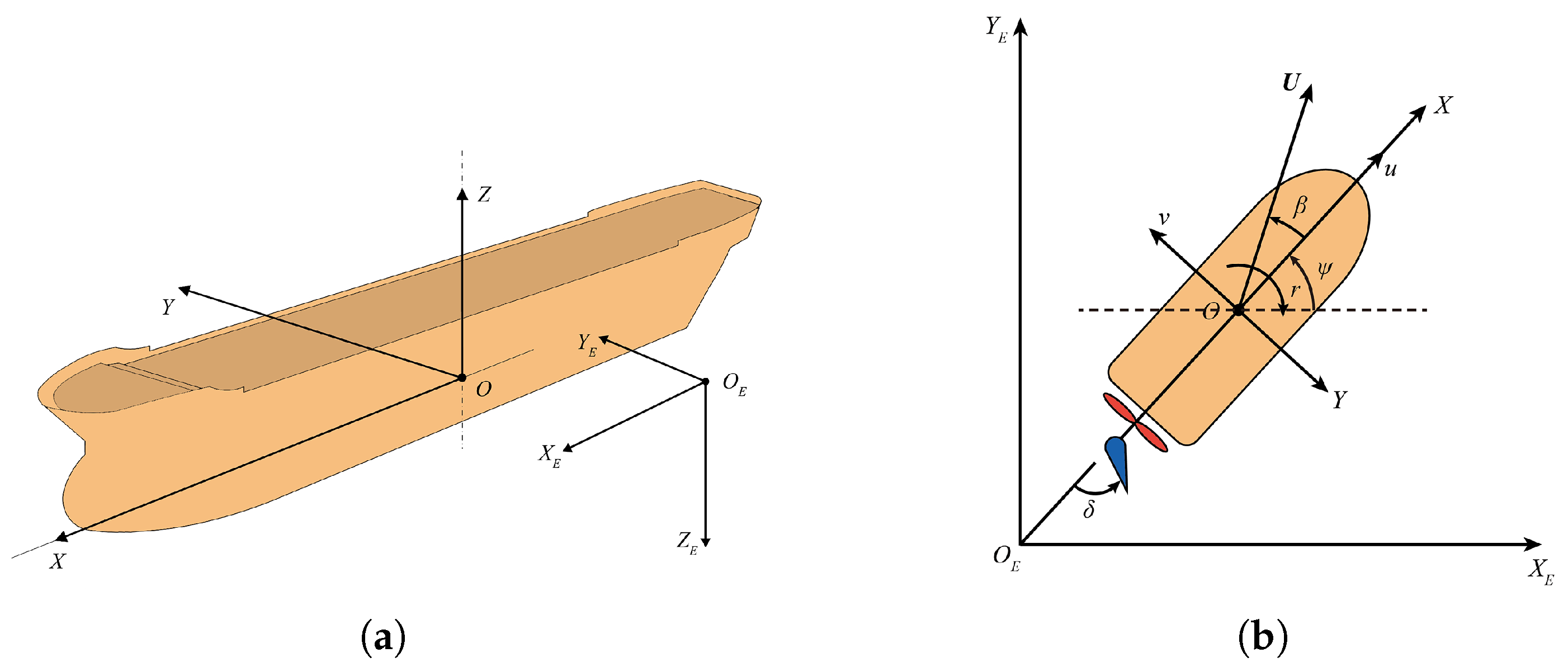
For motion control, it is necessary to first define the state of the ship in the reference coordinate systems. Here, we use the Earth coordinate system $O_E-X_E{Y}_E{Z}_E$ and the body-fixed coordinate system $O-XYZ$ to describe the ship’s motion parameters. As shown in Figure 1a, the Earth coordinate system is established on a tangent plane to the Earth surface, with the x-axis towards the north, the y-axis towards the eas, t and the z-axis perpendicular to the Earth’s surface. In the body-fixed coordinate system, the ASV is treated as a rigid body, with the x-axis towards the bow, the y-axis towards starboard, and the z-axis towards the bottom of the ship. This paper considers a three-DOF mathematical model of ASV operating on the water surface, and the corresponding horizontal reference coordinate systems are illustrated in Figure 1b.

The motion parameters relationship between the two coordinate systems is referred to as the ship kinematic equation, as delineated in Equation (1).

$$\dot{\mathit{\eta }}=J\left(\psi \right)\mathit{\upsilon },$$

(1)

$$J\left(\psi \right)=\left[\begin{array}{ccc}cos\psi & -sin\psi & 0\\ sin\psi & cos\psi & 0\\ 0& 0& 1\end{array}\right],$$

(2)

where $\mathit{\eta }={[x,y,\psi ]}^T$ is the vector of the ship displacements and yaw angle in the Earth coordinate system. $\mathit{\upsilon }={[u,v,r]}^T$ is the vector of the linear and angular velocities and $U=\sqrt{u^2+v^2}$. $J\left(\psi \right)$ is the rotation matrix, as shown in Equation (2). Furthermore, besides the kinematic equation, the dynamic equation is also essential for the control of ASV. The time-domain motion equation is given as follows [20]:

$$M\dot{\mathit{\upsilon }}+C_{RB}\left(\mathit{\upsilon }\right)\mathit{\upsilon }+C_A\left({\mathit{\upsilon }}_r\right){\mathit{\upsilon }}_r+D\left({\mathit{\upsilon }}_r\right){\mathit{\upsilon }}_r=\mathit{\tau }+{\mathit{\tau }}_{wave}+{\mathit{\tau }}_{wind},$$

(3)

where ${\mathit{\upsilon }}_r=\mathit{\upsilon }-{\mathit{\upsilon }}_c\in {\mathbb{R}}^3$ represents the velocity vector of the vessel in relation to the ocean current, which is steady and irrotational. M denotes the total mass matrix. $C_{RB}\left(\mathit{\upsilon }\right)$ is the rigid body Coriolis centripetal force matrix, and $C_A\left({\mathit{\upsilon }}_r\right)$ is the Coriolis centripetal force matrix of the additional mass. $D\left({\mathit{\upsilon }}_r\right)$ refers to the matrix of the water damping coefficients.

$\mathit{\tau }\in {\mathbb{R}}^3$ is the control input vector, and ${\mathit{\tau }}_{wave}$ and ${\mathit{\tau }}_{wind}\in {\mathbb{R}}^3$ correspond to the environmental disturbance forces exerted by wave and wind. Since the left part of Equation (3) incorporates the velocity of the ocean current, there is no need for an additional term of current force. Regarding the control input $\mathit{\tau }$, its relationship with the propeller revolving speed n and rudder angle $\delta$ is illustrated in Equation (4), where C is the configuration matrix of the propellers. $f_c(·)$ is the conversion function [21].

$$\mathit{\tau }=C{f}_c\left({\mathit{\upsilon }}_r,n,\delta \right)$$

(4)

3. Autonomous Navigation and Collision Avoidance Problem Modeling

3.1. Markov Decision Process

As a branch of machine learning, DRL integrates the benefits of both deep learning and RL [22]. The Markov decision process (MDP) is one of the fundamental parts in RL. Here, we define the MDP tuple as $\langle \mathcal{S}$, $\mathcal{A}$, $\mathcal{P}$, $\mathcal{R}$, $\gamma \rangle$, where $\mathcal{S}$ is the set of all environment states, with $s_t\in \mathcal{S}$ indicating the state the agent is in at time t. $\mathcal{A}$ represents the action space. $a_t\in \mathcal{A}$ refers to the action executed by the agent at time t. $\mathcal{P}(s_t,a_t,s_{t+1})\in \mathbb{R}$ represents the probability of the agent transitioning from state $s_t$ to the next state $s_{t+1}$ when taking action $a_t$ in state $s_t$. $\mathcal{R}$ is the reward function, and $r_{t+1}=\mathcal{R}(s_t,a_t)\in \mathbb{R}$ represents the reward the agent received when taking action $a_t$ in state $s_t$. $\gamma \in [0,1]$ is the discount factor [23]. In RL, the policy $\pi$: $\mathcal{S}\to \mathcal{R}$ serves as a function that maps the state space to the action space. Specifically, $\pi \left(a_t\right|s_t)$ represents the probability of selecting action $a_t$ given state $s_t$ under policy $\pi$. Denoting by $G_t$ the discounted cumulative reward at time t, it is calculated by Equation (5).

$$G_t=r_{t+1}+\gamma r_{t+2}+{\gamma }^2{r}_{t+3}+\cdots +{\gamma }^{T-t-1}{r}_T,$$

(5)

where T is the terminal time. The objective of RL is to find an optimal policy to maximize the expected discounted return, which ensures that this return is at least equal to that achieved by any alternative policies [24].

3.2. Path Following and Course Tracking Control

The basis of ASV autonomous navigation is to follow a specified route while avoiding obstacles in complicated environments. Path-following methods, including direct and indirect techniques, are employed to control the motions along a pre-determined path in spatial dimensions without time constraints [25]. The indirect following method is particularly preferred due to its clarity in variable definition and ease of implementation [25].

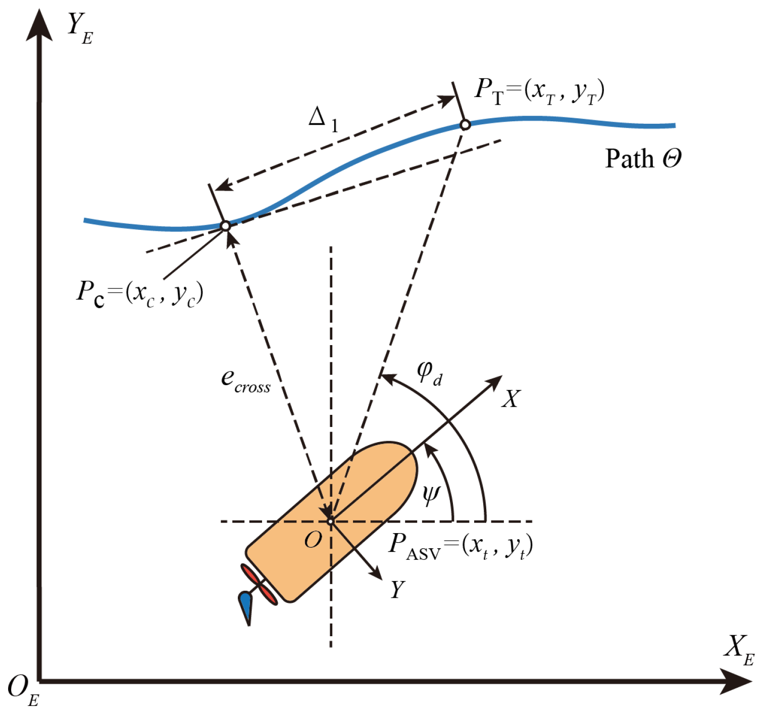
Furthermore, as a key part of ASV guidance and control techniques, the course tracking is a prerequisite for the implementation of indirect path-following control [26]. Figure 2 illustrates the schematic view of indirect path following based on course tracking control, where path $\Theta$ is a line comprising $N_{\Theta }$ discrete points $\{[x_{pi}$, $y_{pi}$${]\}}_{i=1\dots N_{\Theta }}$. ${\Delta }_1$ denotes the forward viewing distance. The ASV first determines the nearest path point $P_c=(x_c,y_c)$ on $\Theta$ relative to its current position with Equation (6), where $P_{\mathit{ASV}}=(x_t,y_t)$ is the ship position. $\left|\right|·{\left|\right|}_2$ is the L2-norm. Then from this nearest path point, the ASV conducts a forward search for a lookout point $P_T=(x_T,y_T)$ along $\Theta$ that is one ${\Delta }_1$ distance away from $P_c$, i.e., $||(x_c,y_c)-(x_T,y_T){||}_2\to {\Delta }_1$. The primary objective of the ASV is to compute the desired course ${\phi }_d$ between the position and the lookout point $P_T$ at each moment t, as shown in Equation (7). It is required to minimize the difference between $\psi$ and ${\phi }_d$ to the greatest extent, i.e., $||\psi -{\phi }_d{||}_2\to 0$.

$$P_c=\underset{(x,y)\in \Theta }{argmin}\left|\right|(x,y)-(x_t,y_t){\left|\right|}_2$$

(6)

$${\phi }_d=atan2\left(y_T-y_t,x_T-x_t\right)$$

(7)

In this study, it is assumed that the rotational speed of a ship propeller remains constant throughout the path-following task. Therefore, at each moment t, the ASV determines an optimal rudder angle ${\delta }_t$ only based on its current position, desired path, and other relevant information to control its heading. This means that the path-following problem satisfies the Markov property and can be addressed using DRL algorithms. In order to improve the policy generalization performance, it is important that the agent’s state space and reward function are designed without the influence of global environmental information. Initially, the controller aims to minimize the deviation between the current heading and the desired course; so, the state space should encompass the yaw angle $\psi$ and the course ${\phi }_d$. Furthermore, since the steering amplitude of the rudder angle in $\Delta t$ should not be excessive, the rudder angle $\delta$ and the angular velocity r are also incorporated into the state representation. Thus, the state vector for the ASV in the path-following task at time t is defined as $s_t=\left[sin{\psi }_t,cos{\psi }_t,sin{\phi }_t,cos{\phi }_t,{\delta }_t,r_t\right]$, while the action vector is $a_t={\delta }_t$.

As for the reward function $r_{p_t}$, it is divided into two components, namely $R_{\mathrm{course}}$ and $R_{\mathrm{rudder}}$. The respective formulations for each reward function are shown in Equations (8) and (9). Equation (10) represents the formula for $r_{p_t}$, where $k_1$ and $k_2$ are both positive weight coefficients. For a given path, the agent continuously obtains a positive reward when the absolute error $|{\psi }_t-{\phi }_{d_t}|$ is small. Conversely, a negative penalty is imposed when the angular error is acute. For $R_{\mathrm{rudder}}$, the penalty diminishes as the amplitude of the rudder angle change within the time $\Delta t$ decreases.

$$R_{\mathrm{course}}={\displaystyle \frac{\pi /2 - |{\psi }_t-{\phi }_{d_t}|}{\pi /2}}$$

(8)

$$R_{\mathrm{rudder}}=-{\displaystyle \frac{\left|{\delta }_{t-1}-{\delta }_t\right|}{\Delta t}}$$

(9)

$$r_{p_t}=k_1·R_{\mathrm{course}}+k_2·R_{\mathrm{rudder}}$$

(10)

3.3. Collision Avoidance Decision-Making

Most of the time the ASV navigates along designated specific routes in open waters and relies only on the path-following controller. However, when it is located in more complex waters, the ASV must implement appropriate measures to avoid obstacles that could lead to a collision. Current collision avoidance algorithms are all local planning methods that must be in real time and consider the dynamic constraints of the vessel [27]. Similar to path-following control, the collision avoidance problem can also be framed as MDP and integrated with DRL for policy optimization.

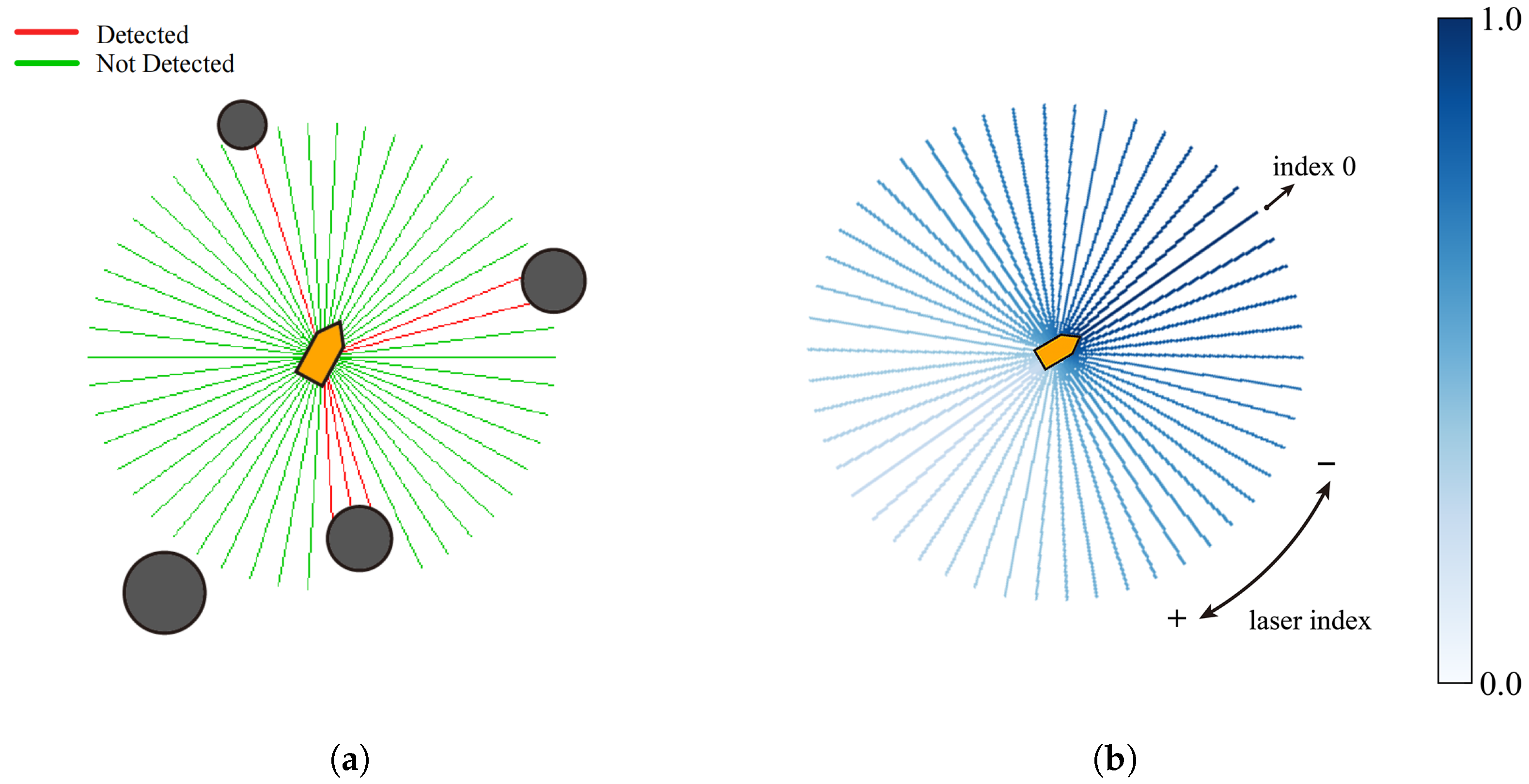
In this paper, the basis of collision avoidance decision-making is LiDAR, a sensor that utilizes laser beams to measure distances and angles, allowing for real-time environment data collection, including the position, shape, and size of obstacles. Figure 3a illustrates a LiDAR on an ASV emitting laser beams in two-dimensional space, where dark circles indicate obstacles, green lines represent laser beams that do not detect any objects, and red lines show beams that make contact with obstacles. Here, we define the maximum detection radius of the LiDAR as $r_{\max }$, the distance between the LiDAR and the point of contact as $r_{\mathrm{obs}}$, and the total number of emitted rays as $N_l$. To ensure our method is suitable for different LiDARs, it is necessary to normalize the detection distances. That is, if a beam i does not hit any obstacles, the detection result should be $r_i=1$. Otherwise the normalized feedback is $r_i=r_{{\mathrm{obs}}_i}/r_{\max }\in [0,1)$.

Specifically, the decision maker first determines the collision avoidance course $\varphi$, which is then used as one of the inputs for the course tracking controller mentioned in Section 3.2. Simultaneously, the propeller revolving speed n is also controlled. Therefore, the agent’s action space consists of the collision avoidance course $\varphi$ and the propeller speed n. Since the ASV needs to avoid collision while approaching its destination, it should take into account not only the feedback information $F=[r_1,r_2,\dots ,r_{N_l}]\in {\mathbb{R}}^{N_l}$ provided by the LiDAR, but also its own yaw angle $\psi$, desired goal course ${\phi }_d$, collision avoidance course $\varphi$, drift angle $\beta$, linear velocity u, v, and angular velocity r. Consequently, the state vector of our decision-making agent at time t stands for $s_t=[F_t,sin{\psi }_t,cos{\psi }_t,sin{\phi }_{d_t},cos{\phi }_{d_t},sin{\varphi }_t,cos{\varphi }_t,sin{\beta }_t,cos{\beta }_t,U_t,r_t]$, and the action vector is $a_t=[{\varphi }_t,n_t]$.

The reward function $r_{o_t}$ for the collision avoidance decision maker is composed of four parts, which are $R_{\mathrm{course}}^{\prime }$, $R_{\mathrm{target}}$, $R_{\mathrm{yaw}}$, and $R_{\mathrm{collision}}$. Specifically, $R_{\mathrm{course}}^{\prime }$ and $R_{\mathrm{target}}$ are designed to assist the ASV approaching $P_T$, which serves as the point guiding the vessel to its destination. Meanwhile, the design of $R_{\mathrm{yaw}}$ aims to prevent excessive changes in the yaw angle. The formulas for calculating $R_{\mathrm{course}}^{\prime }$, $R_{\mathrm{target}}$, and $R_{\mathrm{yaw}}$ are provided below, where $\mathrm{dot}(·)$ is the dot product of two vectors.

$$R_{\mathrm{course}}^{\prime }=\mathrm{dot}\left((\cos {\psi }_t,sin{\psi }_t),(\cos {\phi }_{d_t},sin{\phi }_{d_t})\right)$$

(11)

$$R_{\mathrm{target}}=\left|\right|(x_{t-1},y_{t-1})-P_T{\left|\right|}_2-\left|\right|(x_t,y_t)-P_T{\left|\right|}_2$$

(12)

$$R_{\mathrm{yaw}}=\left\{\begin{array}{cc}-|{\psi }_t-{\psi }_{t-1}|\hfill & \mathrm{if}|{\psi }_t-{\psi }_{t-1}| <\pi \hfill \\ 2\pi - |{\psi }_t-{\psi }_{t-1}|\hfill & \mathrm{otherwise}\hfill \end{array}\right.$$

(13)

For $R_{\mathrm{collision}}$, when the ship collides with an obstacle, it receives a penalty of −1. If none of the lasers detect the obstacle, the reward is 0. If the ship does not collide, but its lasers make contact with the obstacle, the reward is calculated through the weight of each laser beam and the corresponding detection distance. As illustrated in Figure 3b, the laser beam directly in front of the ship is assigned an index of 0, with the indices of other laser beams increasing in a clockwise direction. Additionally, a darker beam color indicates a higher laser weight value. The equations for computing the laser weight $W\in {\mathbb{R}}^{N_l}$ are shown in Equations (14) and (15), where $k_3$ is a small negative constant, and ${\chi }_i\in [0,N_l)$ represents the index of the laser beam i. The formula for $R_{\mathrm{collision}}$ is shown in Equation (16), where $\mathbb{1}$ denotes the unit vector.

$$w_i=\left\{\begin{array}{cc}exp\left[k_3·\left(N_l-{\chi }_i\right)\right]\hfill & \mathrm{if}\left(N_l\mathrm{is}\mathrm{even}\bigcap {\chi }_i>N_l/2\right)\bigcup \left(N_l\mathrm{is}\mathrm{odd}\bigcap {\chi }_i>(N_l-1)/2\right)\hfill \\ exp\left(k_3·{\chi }_i\right)\hfill & \mathrm{otherwise}.\hfill \end{array}\right.$$

(14)

$$W=\left[w_1,w_2,\dots ,w_{N_l}\right],w_{i=1,\dots ,N_l}\in [0,1]$$

(15)

$$R_{\mathrm{collide}}=\left\{\begin{array}{cc}-1\hfill & \mathrm{if}\mathrm{collide}\hfill \\ 0\hfill & \mathrm{if}\min \left(F_t\right)=1\hfill \\ W_t{(F_t-\mathbb{1})}^T\hfill & \mathrm{otherwise}.\hfill \end{array}\right.$$

(16)

According to the previously mentioned formulas, if there are obstacles directly in front of the ship, the agent will receive a larger negative reward than that of the situation when obstacles are located in other directions, as the obstacles ahead present a higher risk of collision. The total reward function $r_{o_t}$ can be expressed as Equation (17), where $k_4, k_5, k_6,$ and $k_7$ are all positive weight coefficients.

$$r_{o_t}=k_4·R_{\mathrm{course}}^{\prime }+k_5·R_{\mathrm{target}}+k_6·R_{\mathrm{yaw}}+k_7·R_{\mathrm{collide}}$$

(17)

4. Autonomous Navigation and Collision Avoidance Methods Based on Deep Reinforcement Learning

4.1. Soft Actor–Critic Algorithm

For an RL agent in state s at time t, we denote the expected discounted return with respect to the policy $\pi$ as $V_{\pi }\left(s\right)$. For the agent taking action a in state s at time t, the expected return is expressed as $Q_{\pi }(s,a)$ [23]. The corresponding formulas are shown in Equations (18) and (19).

$$\begin{array}{c}\hfill V_{\pi }\left(s\right)={\mathbb{E}}_{\pi }\left[G_t|s_t=s\right]\end{array}$$

(18)

$$\begin{array}{c}\hfill Q_{\pi }(s,a)={\mathbb{E}}_{\pi }\left[G_t|s_t=s,a_t=a\right]\end{array}$$

(19)

This paper utilizes the SAC to train the DRL policy. The SAC is a state-of-the-art DRL algorithm that employs the Actor–Critic framework and learns a stochastic policy while incorporating a regularization term to enhance exploration capabilities [28]. It uses a total of five networks, including one actor network $\pi$ with parameter $\theta$, two critic networks: $Q_1$ with parameter ${\omega }_1$ and $Q_2$ with parameter ${\omega }_2$, and two target critic networks: ${\widehat{Q}}_1$ with parameter ${\omega }_1^{-}$ and ${\widehat{Q}}_2$ with parameter ${\omega }_2^{-}$. Since the SAC is an off-policy based DRL algorithm, it maintains a replay buffer $\mathcal{D}$ for policy training. The actor and critics are updated through gradient back propagation, as shown in Equations (20) and (21).

$$\theta \leftarrow \theta -\lambda {\nabla }_{\theta }{\mathbb{E}}_{s\sim \mathcal{D},a\sim \pi (·|s)}\left[\alpha log\pi \left(a\right|s)-{min}_{k=1,2}{Q}_k(s,a)\right]$$

(20)

$${\omega }_j\leftarrow {\omega }_j-\lambda {\nabla }_{{\omega }_j}{\displaystyle \frac{1}{2}}{\mathbb{E}}_{s,a\sim \mathcal{D}}{\left[Q_j(s,a)-r(s,a)-\gamma {\mathbb{E}}_{s^{\prime }\sim \mathcal{P}(·|,a),a^{\prime }\sim \pi (·|s^{\prime })}{min}_{k=1,2}{\widehat{Q}}_k(s^{\prime },a^{\prime })\right]}^2,j=1,2,$$

(21)

where $\lambda$ is the learning rate. $\alpha$ is the regularization coefficient. The target critics are soft updated at specific intervals, as shown in Equation (22), where $\zeta$ represents the soft update coefficient.

$${\omega }_j^{-}\leftarrow \zeta {\omega }_j+\left(1-\zeta \right){\omega }_j^{-},j=1,2$$

(22)

4.2. Autonomous Navigation Control and Collision Avoidance Decision-Making Method

4.2.1. Policies Training

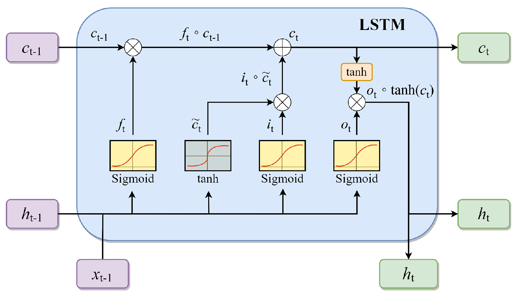
For the path-following agent, the LSTM module is introduced to improve its prediction ability considering the delay in ship maneuvering. As illustrated in Figure 4, the LSTM features a unique memory cell and gate mechanism that effectively captures and processes long short-term dependencies in sequential data [29]. Therefore, the past state series $s_{t-N_s}$, $s_{t-N_s+1}$, …, $s_{t-1}$ along with the current state $s_t$ are input to the LSTM layer to extract time series features, which enables the ASV to forecast its own state. The output from the LSTM is then used as the input for next layers in the model. For the collision avoidance policy, the ASV is trained in a setting with randomly placed static obstacles. The LiDAR first emits $N_l$ beams of laser with the ship’s current position as the center. It then iterates each beam to generate a feedback list F. The agent combines its motion parameters and list F to compute the current state $s_t$. The policy is also developed using the SAC algorithm, incorporating LSTM module to improve the agent’s predictive capability.

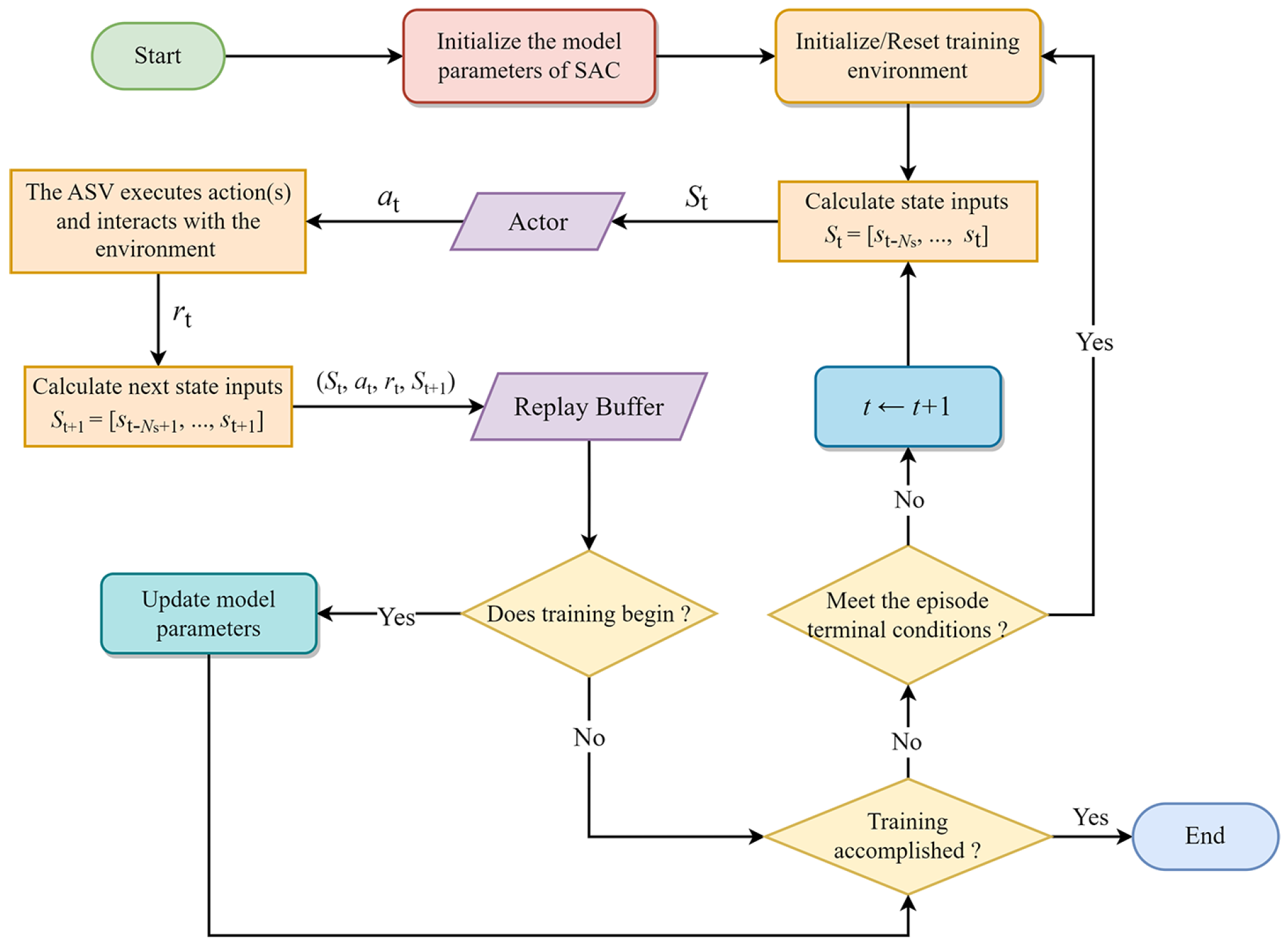
Figure 5 shows the flowchart of the policy training process. The agent interacts with the environment by taking action(s) and receives rewards at each time step; then, it updates the current state and determines whether the episode is terminated or not. In the case of the path-following policy, if the ship arrives at the target point, the maximum time step is reached, or the ship exceeds the map boundaries, the current episode is terminated, and the next new episode will commence. Whereas for the collision avoidance policy, besides the condition for the distance between the ASV and the target point, the episode also ends if the maximum time step is reached without any collisions.

4.2.2. Trajectory Prediction of Dynamic Obstacle

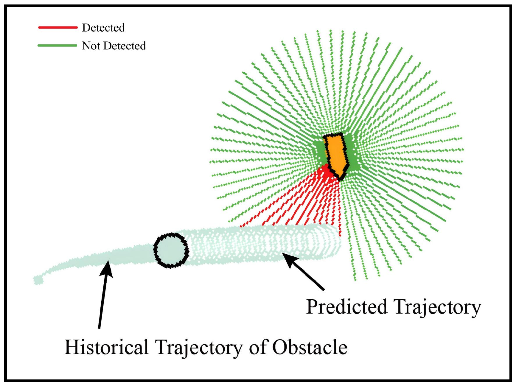
Since the collision avoidance policy is trained in an environment with static obstacles, applying the policy directly to dynamic scenarios for ASV may not yield ideal results. As illustrated in Figure 6, it is assumed that the historical data of dynamic obstacles’ coordinates within the map area are accessible to the ASV, allowing it to forecast the future trajectories of obstacles. In addition, all the predicted trajectory points are treated as imagined obstacles for the ASV to avoid potential collisions.

The Kalman filter (KF) is a widely used algorithm for estimating states and is composed of three steps: measurement, state update, and prediction [30]. In this paper, we apply an improved KF algorithm for short-term predictions of motion trajectories with the kinematic model of dynamic obstacles [31]. Here, the state vector X is defined as $X={\left[x,u,a_x,y,v,a_y\right]}^T$, where x, y are the positions. u, v are the linear velocities, and $a_x$, $a_y$ are the linear accelerations, all referenced in the Earth coordinate system. The state extrapolation equation is presented in Equation (23).

$$X_{t+1}=A{X}_t+B{u}_t+E{\tilde{j}}_t,$$

(23)

where $X_t$ is the state at time t. $u_t\in {\mathbb{R}}^2$ is the control input. ${\tilde{j}}_t\in {\mathbb{R}}^2$ is the noise. A is the state transition matrix. B is the control matrix, and E is the noise matrix. According to the kinematic model, the expressions for A, B, and E are shown in Equation (24), Equation (25), and Equation (26), respectively. Since both $u_t$ and ${\tilde{j}}_t$ are taken as the acceleration rates in this paper, the original state equation Equation (23) can be reformed as Equation (27).

$$A=\left[\begin{array}{cc}{A}_x& 0\\ 0& A_y\end{array}\right]$$

(24)

$$A_x=A_y=\left[\begin{array}{ccc}1& \Delta t& {\displaystyle \frac{\Delta t^2}{2}}\\ 0& 1& \Delta t\\ 0& 0& 1\end{array}\right]$$

(25)

$$B=E={\left[\begin{array}{cccccc}{\displaystyle \frac{\Delta t^3}{6}}& {\displaystyle \frac{\Delta t^2}{2}}& \Delta t& 0& 0& 0\\ 0& 0& 0& {\displaystyle \frac{\Delta t^3}{6}}& {\displaystyle \frac{\Delta t^2}{2}}& \Delta t\end{array}\right]}^T$$

(26)

$$X_{t+1}=A{X}_t+B(u_t+{\tilde{j}}_t)$$

(27)

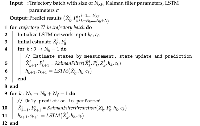
We denote the new control vector at time t as ${\tilde{u}}_t=u_t+{\tilde{j}}_t$, with its covariance represented as $q_{{\tilde{u}}_t}$, its estimated value as ${\widehat{\tilde{u}}}_t$, and the covariance of its estimated value as $q_{{\widehat{\tilde{u}}}_t}$. In the KF prediction stage, we define the predicted state and covariance at time t as ${\widehat{X}}_t$ and $P_t$; then, the state ${\widehat{X}}_{t+1}$ and covariance $P_{t+1}$ at time $t+1$ are calculated through Equations (28) and (29). Since what the ASV can have access to is the coordinates data of obstacles, for ${\widehat{\tilde{u}}}_t$ and $q_{{\widehat{\tilde{u}}}_t}$, they are predicted by an additional LSTM unit in this paper. We denote the output $h_t$ of LSTM at time t as $h_t=[{\widehat{\tilde{u}}}_t,q_{{\widehat{\tilde{u}}}_t}]$. Then, we have Equation (30).

$${\widehat{X}}_{t+1}=A{\widehat{X}}_t+B{\widehat{\tilde{u}}}_t$$

(28)

$$P_{t+1}=A{P}_t{A}^T+B{q}_{{\widehat{\tilde{u}}}_t}{q}_{{\widehat{\tilde{u}}}_t}^T{B}^T$$

(29)

$$h_t,c_t=\mathit{LSTM}\left({\widehat{X}}_{t-1},h_{t-1},c_{t-1}\right)$$

(30)

$$\sigma \leftarrow \underset{\sigma }{\mathrm{argmin}}\mathit{MSE}\left(\mathit{Predict}\left(N_h,\sigma \right),N_f\right)$$

(31)

Let the LSTM parameter be $\sigma$. To train the network, we assume there is a database ${\mathcal{D}}_{\mathit{KF}}$ containing the trajectories of moving objects. Then, we sample a batch of trajectories with the size of $N_{\mathit{KF}}$. Each trajectory is split into a historical segment with a horizon of $N_h$ and a future segment with a horizon of $N_f$. Then, the predicted values from the LSTM model based on the points within $N_h$, i.e., $\mathit{Predict}\left(N_h,\sigma \right)$, are compared to the future observations within $N_f$ by calculating the mean squared error (MSE) loss. The network parameters are then updated through back-propagation, as shown in Equation (31).

The KF executes measurement, state update, and prediction repeatedly to estimate states [30]. In this paper, the KF is initialized using historical observations from time 0 to $N_h-1$ as usual. However, after time $N_h-1$, only the prediction step is performed without utilizing any future observations within the horizon of $N_f$. As illustrated in Algorithm 1, with the KF initialized using the historical data, the state and covariance estimates at time $N_h$ are used as the initial values for trajectory prediction, which is based on Equations (28) and (29).

Algorithm 1: KF-LSTM Algorithm

4.2.3. Hybrid Autonomous Navigation and Collision Avoidance System in Complex Environments

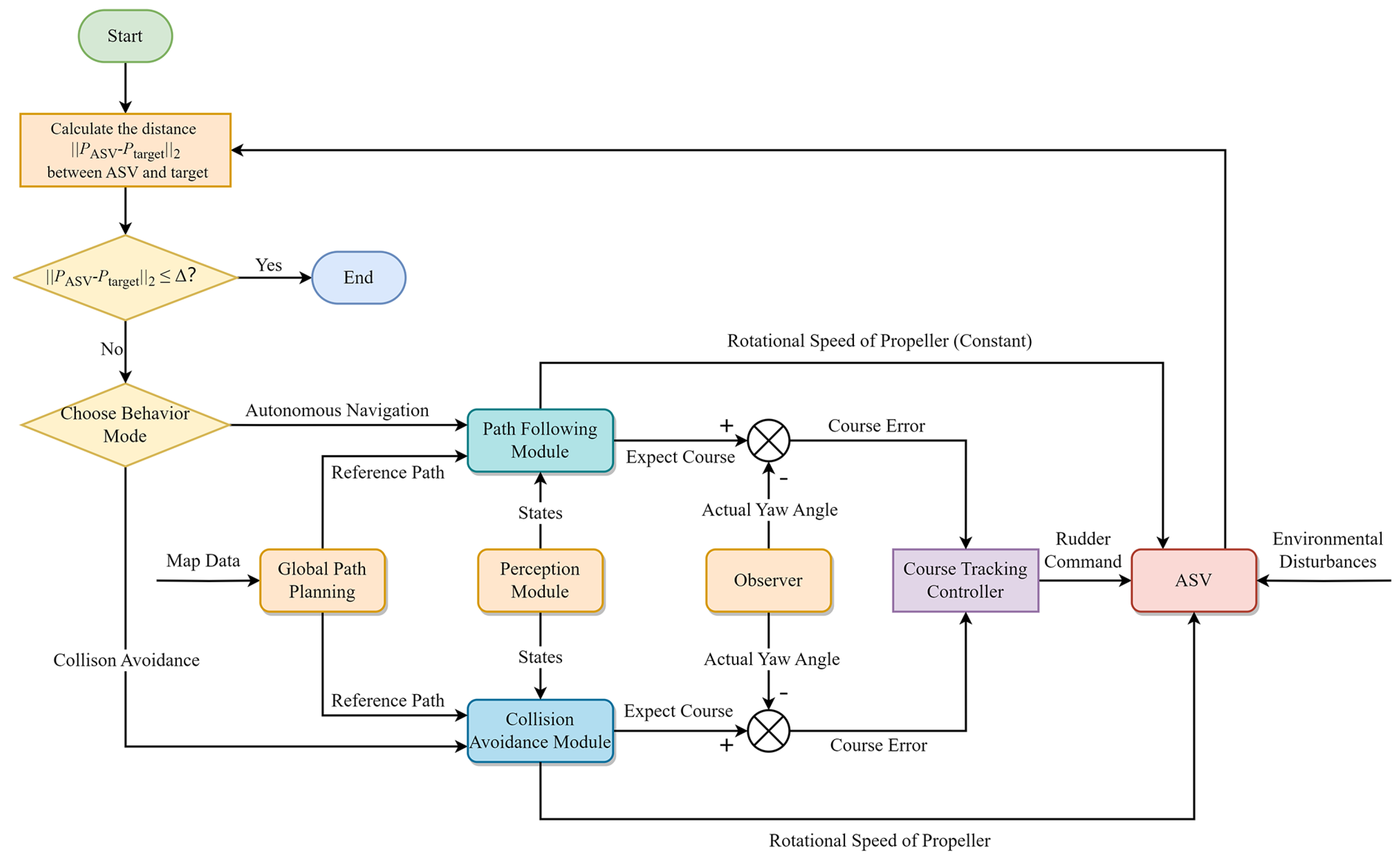
The flowchart of the system is illustrated in Figure 7. In practice, the ASV encounters various static and dynamic obstacles. It is also affected by external factors like wind, wave, and current. For navigation in a complex environment, the vessel first conducts global path planning with map data to generate a feasible collision-free path from the starting point to the destination. The path can be designed either manually or through global path planning algorithms. Once a collision-free path is determined, in the path-following module, the ASV continuously updates local lookout points $P_T$ and calculates the desired course ${\phi }_d$ at each moment. Subsequently, the angular error is calculated and fed into the course tracking controller, which produces control commands to steer the vessel safely along the designated path.

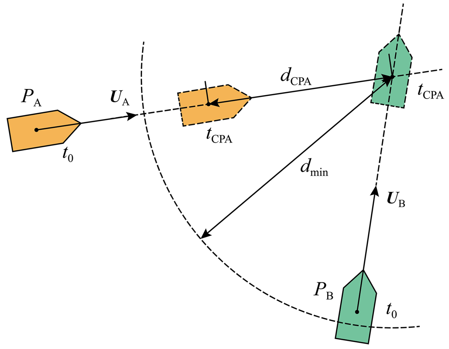
The criterion for switching policies is based on the collision risk. When the vessel does not identify any dynamic obstacles during its navigation, the system defaults to autonomous navigation mode to follow the pre-defined path. Otherwise, it shifts to collision avoidance mode. Here, we introduce the concept of the closest point of approach (CPA) as a metric for evaluating the collision risk [32]. As shown in Figure 8, $P_A$ represents the coordinates of the ASV. $P_B$ denotes the coordinates of the dynamic obstacle. The vector ${\mathit{\upsilon }}_A$, ${\mathit{\upsilon }}_B\in {\mathbb{R}}^2$ corresponds to the linear velocities in the Earth coordinate system. At time $t_{\mathit{CPA}}$, both the ASV and the obstacle reach their respective CPA simultaneously, maintaining a distance of $d_{\mathit{CPA}}$ to their encounter points. The formulas for $t_{\mathit{CPA}}$ and $d_{\mathit{CPA}}$ are shown in Equation (32) and Equation (33), respectively.

$$t_{\mathit{CPA}}={\displaystyle \frac{(P_B-P_A)·({\mathit{\upsilon }}_A-{\mathit{\upsilon }}_B)}{\left|\right|{\mathit{\upsilon }}_A-{\mathit{\upsilon }}_B{\left|\right|}_2}}$$

(32)

$$d_{\mathit{CPA}}=\left|\right|(P_A+{\mathit{\upsilon }}_A{t}_{\mathit{CPA}})-(P_B+{\mathit{\upsilon }}_B{t}_{\mathit{CPA}}){\left|\right|}_2$$

(33)

When the ASV satisfies both $0\le t_{\mathit{CPA}}\le t_{max}$ and $d_{\mathit{CPA}}\le d_{min}$, it indicates a potential collision risk. At this time, the ship predicts the trajectory of dynamic obstacles, avoiding virtual and actual obstacles at the same time. It is worth noting that in collision avoidance mode, the forward viewing distance ${\Delta }_2$ to search for a local lookout point along the global path needs to exceed ${\Delta }_1$ in path following to avoid urgent maneuvers.

5. Results and Discussion

5.1. The Parameters Setting

The parameters of the ASV adopted in the present study are defined based on a 1:300 model-scale VLCC with a single propeller and a single rudder. The mass m of the model is 10 kg. The overall length $L_{OA}$ of the model is 1.11 m, and the width B is 0.165 m. The major parameters of this model-scale vessel are detailed in

Table 1. Major parameters of the model-scale VLCC.

Parameter	Unit	Value
Overall length	m	1.11
Overall width	m	0.165
Draft	m	0.068
Displacement	kg	10
$X_g$	m	0.562
$Y_g$	m	0
$Z_g$	m	0.058
$R_{xx}$	m	0.052
$R_{yy}$	m	0.26
$R_{zz}$	m	0.26

. Since the revolution speed of the propeller is proportional to the pulse-width modulation ($\mathrm{PWM}$) of the motor, the PWM value is used to replace the revolution speed n with a range of $\mathrm{PWM}\in [-100,100]$. The permissible range for the rudder angle is $\delta \in [-30\mathrm{deg},30\mathrm{deg}]$. Additionally, the hardware used for the algorithm training is NVIDIA RTX 4080 GPU. PyTorch 2.1 is also used, and the environment is built on OpenAI gym. Based on the current hardware and computational capability, the average inference time per step of the proposed policy is less than 50 ms, which can meet the real-time requirement for the ASV.

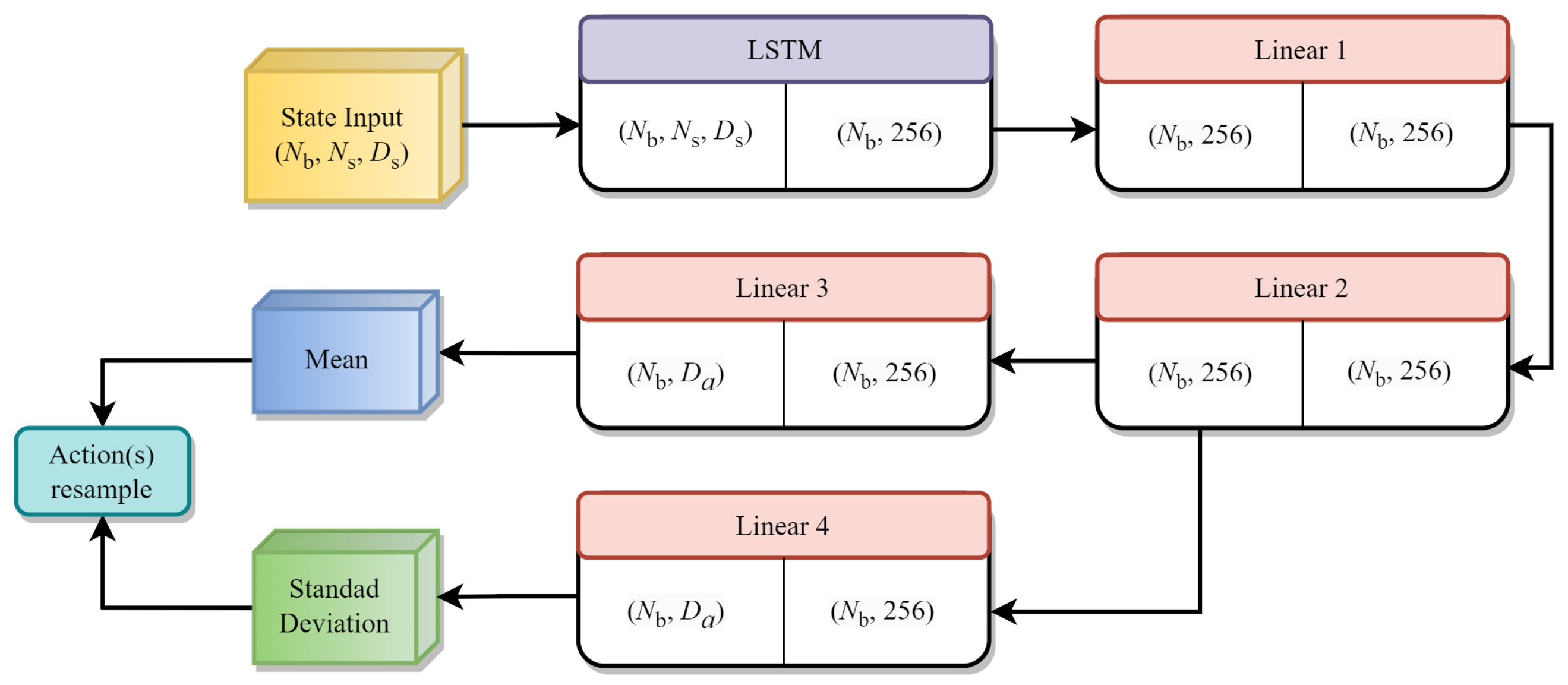
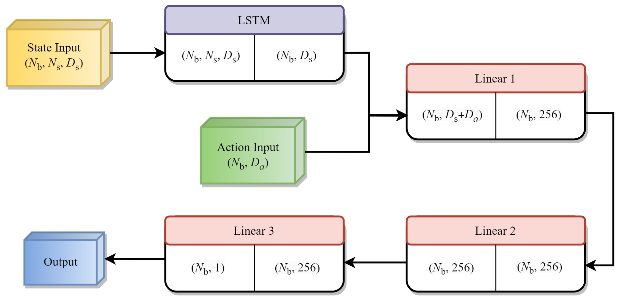
Other algorithm parameters and the network structure of actor and critics in policy are shown in

Table 2. Hyperparameters of algorithms.

Parameter	Value	Parameter	Value
Time step $\Delta t$ (s)	0.5	Learning rate $\lambda$	3 × 10−4
Soft-update coefficient $\zeta$	5 × 10−3	Batch size of policy training $N_b$	256
Batch size of KF-LSTM training $N_{\mathit{KF}}$	128	Discount factor $\gamma$	0.99
Actor and critic network update interval	1	Target network update interval	1
Policy training start step	1 × 104	Replay buffer size	1 × 106
Historical states horizon $N_s$	6	KF-LSTM historical horizon $N_h$	8
KF-LSTM prediction horizon $N_f$	30	Maximum CPA time $t_{max}$ (s)	50
Minimum CPA distance $d_{min}$ (m)	200	Threshold distance $\Delta$ (m)	10.0
Forward viewing distance ${\Delta }_1$ (m)	8.0	Forward viewing distance ${\Delta }_2$ (m)	30.0
Coefficient $k_1$	1.0	Coefficient $k_2$	1.0
Coefficient $k_3$	−0.1	Coefficient $k_4$	1.0
Coefficient $k_5$	1.0	Coefficient $k_6$	0.6
Coefficient $k_7$	5.0	-	-

and Figure A1, respectively. In the path-following task, the values of $k_1$ and $k_2$ are set to the same positive value. For the collision avoidance task, the coefficient $k_7$ should have the highest value to impose a large penalty when the ASV is close to or collides with obstacles. Both $k_4$ and $k_5$ pertain to the ASV approach to the target point and should be greater than $k_6$, which is relatively less important during navigation. The simulation environment for the training of path following and the collision avoidance policy is a 1280 m × 720 m collision-free open water. During policy training and verifying, the starting point and the target point of the ASV are both randomly initialized at the start of each episode. All the factors in original velocity vector ${\mathit{\nu }}_0={[u_0,v_0,r_0]}^T$ are set to 0.

5.2. Training Results and Discussion

5.2.1. Path-Following Policy

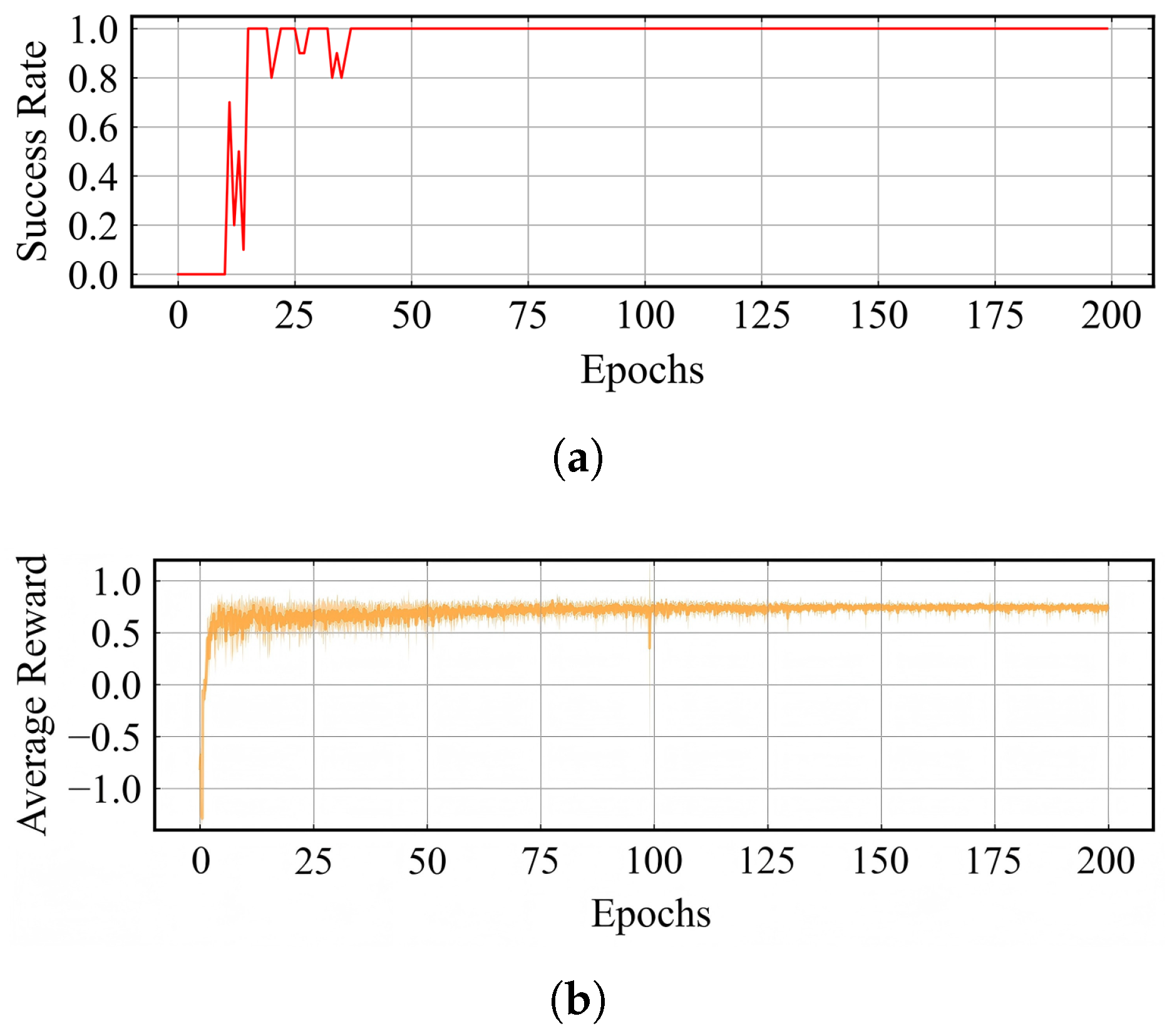
The policy is trained for a total of 2,000,000 iterative steps, with each 1000 steps counted as one epoch. Model parameters of the actor are saved after each epoch, and the model is then verified over 10 episodes to assess the success rate and average reward per step of the agent. The initial yaw angle of the ASV is randomized before the start of episode, and the PWM is 80. To illustrate the training process of the policy, Figure 9 shows the ship trajectory with examples of three different training stages in which the starting point and the target point are fixed. In Figure 9a, the ASV possesses an entire stochastic policy, and there is no trajectory that arrives at the target point. With the increase in the training epoch, the ASV gradually learns how to complete the path-following task shown in Figure 9b, and all of the trajectories reach the destination shown in Figure 9c. Figure 10a displays the ratio of the successful arrival episodes to the target point out of the total episodes in the first 200 epochs. The “success” here indicates that the ASV can arrive at the target point. Figure 10b illustrates the the average reward and standard deviation for each step throughout the entire validation process. Notably, in the first 50 epochs, the success rate experiences considerable fluctuations, showing the inherent performance of the DRL-based path-following policy, while the average reward per step keeps increasing. In the subsequent epochs, the success rate levels off at 1. Additionally, the variance of the average reward decreases continuously, with the mean value eventually stabilizing around 0.7.

5.2.2. Collision Avoidance Policy

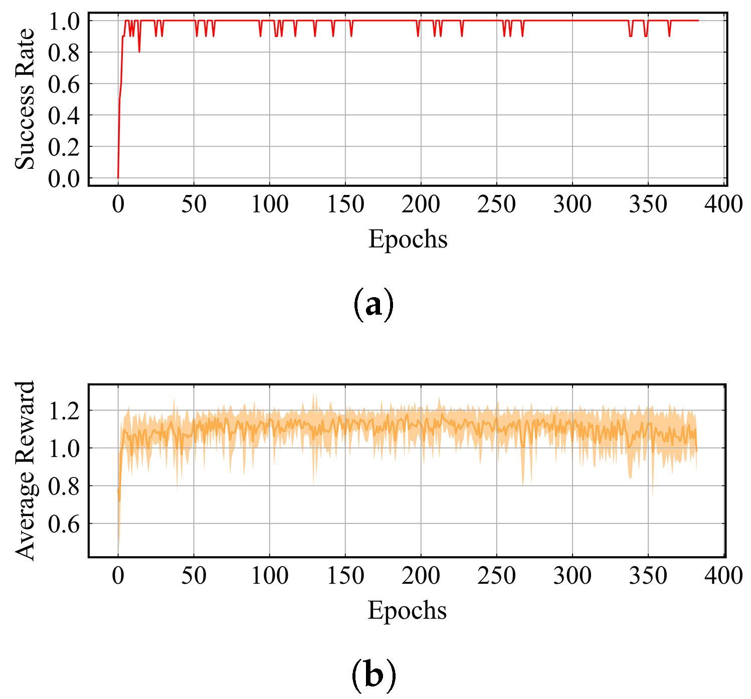
In this section, the number of static obstacles in the training environment is 25 with a radius range of [7 m, 12 m]. The maximum detection radius $r_{max}$ of LiDAR is 70 m, and the number of laser beams $N_l$ is 64. The initial yaw angle is fixed as the angle between the starting point and target point. The collision avoidance policy is trained for a total of 5,000,000 iterative steps, with every five episodes considered as one epoch. The actor parameters are also saved after each epoch with the model validated over 10 episodes.

Similar to Figure 9, ship trajectories from three different training stage are shown in Figure 11. The obstacles, the starting point, and the target point remain unchanged. It is obvious that although most of the trajectories in Figure 11 successfully arrive at the target point, the trajectories in Figure 11c are more compact than those from earlier epochs. Figure 12a shows the success rate of the ASV, and Figure 12b presents the average reward and standard deviation for each step. The success rate quickly rises to 1.0 within a few epochs and stabilizes between 0.9 and 1.0 during training. The average reward per step also stabilizes rapidly between 1.0 and 1.2, albeit with distinct fluctuations in the standard deviation.

5.2.3. KF-LSTM Predictor

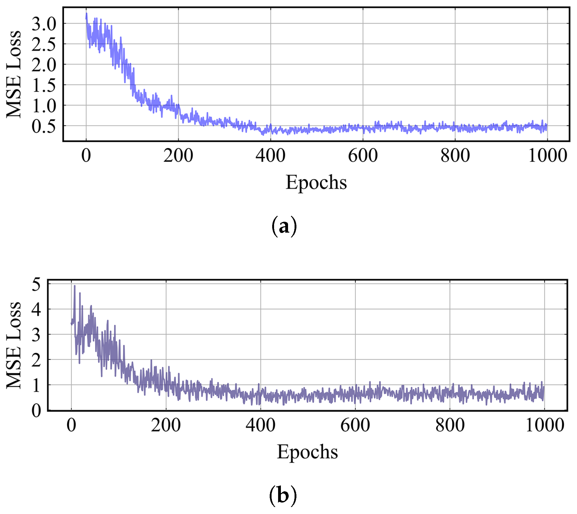
Here, we utilize a publicly accessible ship AIS dataset provided by the Danish Maritime Authority as ${\mathcal{D}}_{\mathit{KF}}$ for the training of the KF-LSTM predictor model [33]. Figure 13 visualizes the AIS dataset, which includes a total of 11,888 navigation trajectories, with each trajectory containing the ship’s Maritime Mobile Service Identity (MMSI) code, time steps, longitudes, latitudes, headings, and velocities. The sampling batch size $N_{\mathit{KF}}$ is 128, with a total of 1000 epochs trained. The model structure contains one LSTM hidden layer with a hidden size of 60. Figure 14 separately shows the change in the MSE error during the training and validation process, indicating a generally decreasing trend from epochs 0 to 200. As the number of epochs increases further, the average training loss ultimately converges to approximately 0.5 and shows less fluctuation than the average validation loss, which stabilizes between 0 and 1.

5.3. Experimental Results and Discussion

5.3.1. Circular Path-Following Simulations

In this subsection, we further test the performance of our path-following policy using two scenarios involving the same circular path. The vessel first navigates along a straight segment before completing a full loop of a circular path. The coordinates of the starting point are (440 m, 300 m), and those of the target point are (439 m, 169 m), with the PWM of ASV fixed at 80. The environmental disturbances are considered in this subsection, including wind, current and wave.

Equation (34) presents the wind load exerted on a structure [34], where ${\rho }_a$ denotes the air density. $U_R$ indicates the relative wind speed. ${\alpha }_R$ signifies the relative wind angle. $A_f$ refers to the front ship projection area, and $A_s$ is the lateral projection area of the ASV above the waterline. $C_{x_{wind}}$, $C_{y_{wind}}$, and $C_{n_{wind}}$ are the wind load coefficients. These wind load coefficients are obtained by the use of standard CFD wind load simulations, which can be seen in Figure 15.

$${\mathit{\tau }}_{wind}={\displaystyle \frac{1}{2}}{\rho }_a{U}_R^2\left[\begin{array}{c}{A}_f{C}_{x_{wind}}\left({\alpha }_R\right)\\ A_s{C}_{y_{wind}}\left({\alpha }_R\right)\\ A_s{L}_{OA}{C}_{n_{wind}}\left({\alpha }_R\right)\end{array}\right]$$

(34)

For the wave load, only the second-order drift forces and moment are considered, and the empirical equations are shown in Equation (35) [35].

$${\mathit{\tau }}_{wave}={\rho }_{c}g{L}_{OA}\left[\begin{array}{c}\cos \left(\vartheta \right){\int }_0^{\infty }S\left(\omega \right)C_{x_{wave}}\left({\lambda }_{\omega }\right)d\omega \\ \sin \left(\vartheta \right){\int }_0^{\infty }S\left(\omega \right)C_{y_{wave}}\left({\lambda }_{\omega }\right)d\omega \\ \sin \left(\vartheta \right)L_{OA}{\int }_0^{\infty }S\left(\omega \right)C_{n_{wave}}\left({\lambda }_{\omega }\right)d\omega \end{array}\right],$$

(35)

where ${\rho }_c$ denotes the fluid density. g is the gravity acceleration. $\vartheta$ represents the encounter angle of the wave. $\omega$ is the wave circular frequency, and ${\lambda }_{\omega }$ is the wavelength corresponding to the frequency $\omega$. $S\left(\omega \right)$ is the wave spectral density. In this paper, the spectrum is adapted from [36]. $C_{x_{wave}}$, $C_{y_{wave}}$, and $C_{n_{wave}}$ are the coefficients of the wave loads. The specific values of the environmental parameters in the simulation are detailed in

Table 3. Parameters of environmental disturbances.

Parameter	Value	Parameter	Value
Wind speed $U_W$ (m/s)	1.5	Wind angle ${\alpha }_W$ (rad)	−3$\pi$/4
Wave angle $\vartheta$ (rad)	−3$\pi$/4	Current speed ${\upsilon }_c$ (m/s)	0.2
Current angle ${\psi }_c$ (rad)	−3$\pi$/4	Air density ${\rho }_a$ (kg/${\mathrm{m}}^3$)	1.29
Fluid density ${\rho }_c$ (kg/${\mathrm{m}}^3$)	1030	Gravitational acceleration g (m/${\mathrm{s}}^2$)	9.8
Frontal projection area $A_f$ (${\mathrm{m}}^2$)	0.0066	Lateral projection area $A_s$ (${\mathrm{m}}^2$)	0.0444

. These environmental parameters are selected based on the upper limit of the small-scale VLCC thrust forces in order to show its performance in a harsh sea environment.

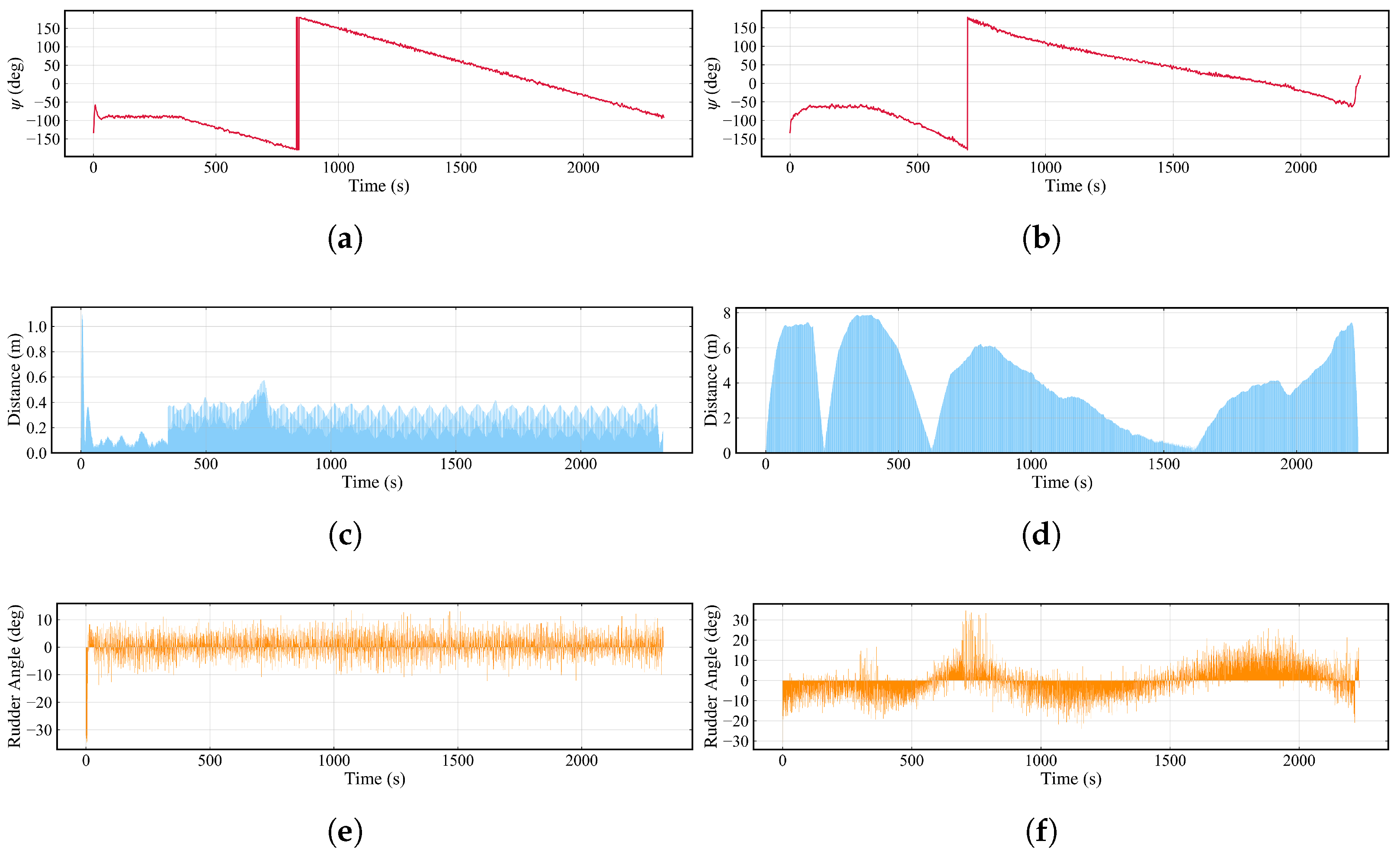
Figure 16a provides schematic view of the process in a static water environment (Scenario $\mathrm{I}$), whereas Figure 16b depicts the scenario in an environment subject to disturbances (Scenario $\mathrm{II}$), which includes the forces and moments of wind, current, and wave. Figure 17 shows the change in the yaw angle, the distance error between the actual path and global path, and the rudder angle over time in the two environments.

Table 4. The path-following errors in scenarios $\mathrm{I}$ and $\mathrm{II}$.

Parameter	Value	Parameter	Value
Average error in Scenario $\mathrm{I}$ (m)	0.210	Average error in Scenario $\mathrm{II}$ (m)	3.979
Maximum error in Scenario $\mathrm{I}$ (m)	1.098	Maximum error in Scenario $\mathrm{II}$ (m)	7.886
Time for maximum error in Scenario $\mathrm{I}$ (s)	5.5	Time for maximum error in Scenario $\mathrm{II}$ (s)	396.5

lists the path-following errors for the whole process. In the static environment, the path error initially reaches a maximum of 1.098 m. At this point, the rudder is significantly adjusted to realign the yaw angle to −90 deg, which corresponds to the direction of the local target point on the straight line segment. Subsequently, the path deviation on this segment is minimal, and then it fluctuates between 0.2 to 0.4 m on the circular path. The rudder angle remains stable within a range of −10 to 10 deg, and the heading transitions smoothly in accordance with the curvature of the circular path. For the task in another environment with disturbances, the average deviation is higher than that of a static environment at 3.979 m, and the maximum error is 7.886 m at 396.5 s. Additionally, the changes in heading and rudder steering behavior exhibit significant differences, attributable to the disturbances present in this environment.

5.3.2. Model Tests of Autonomous Navigation Method

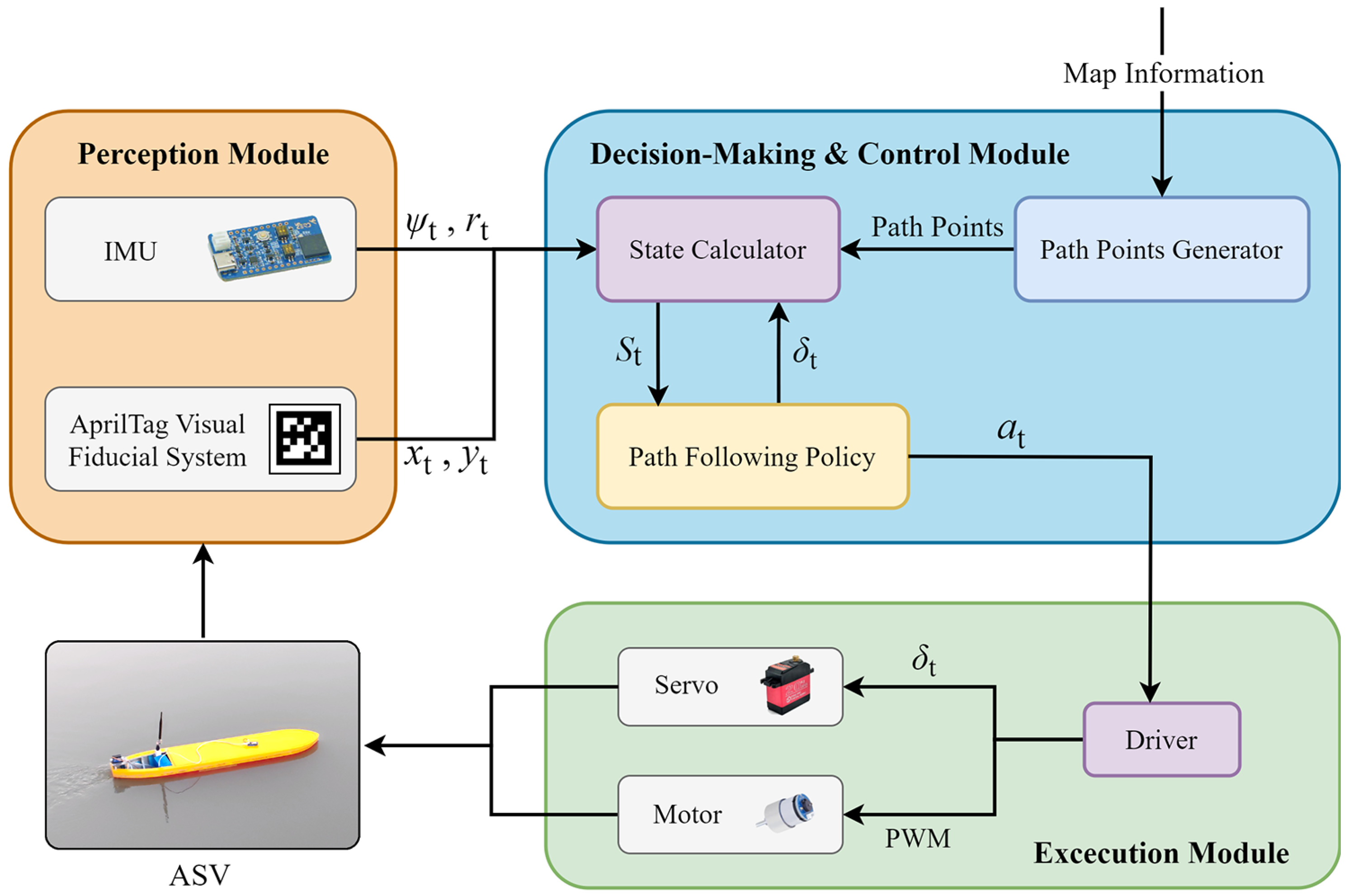
Model tests are conducted in this section to evaluate the performance of our autonomous navigation method based on the path-following policy. As illustrated in Figure 18, the prototype system comprises a VLCC ship model, a perception module that incorporates an inertial measurement unit (IMU) and an AprilTag visual recognition system, a decision-making and control module that includes a path points generator, a state calculator, and a path-following policy, and an execution module including a driver, a servo, and a motor.

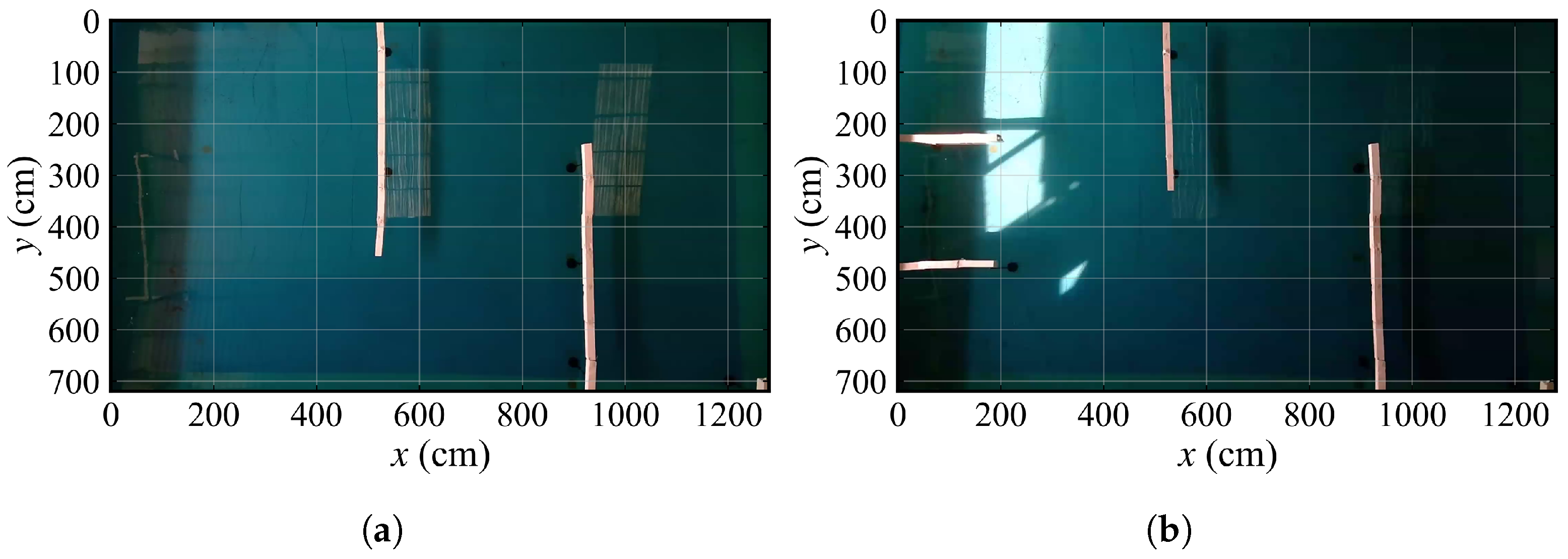
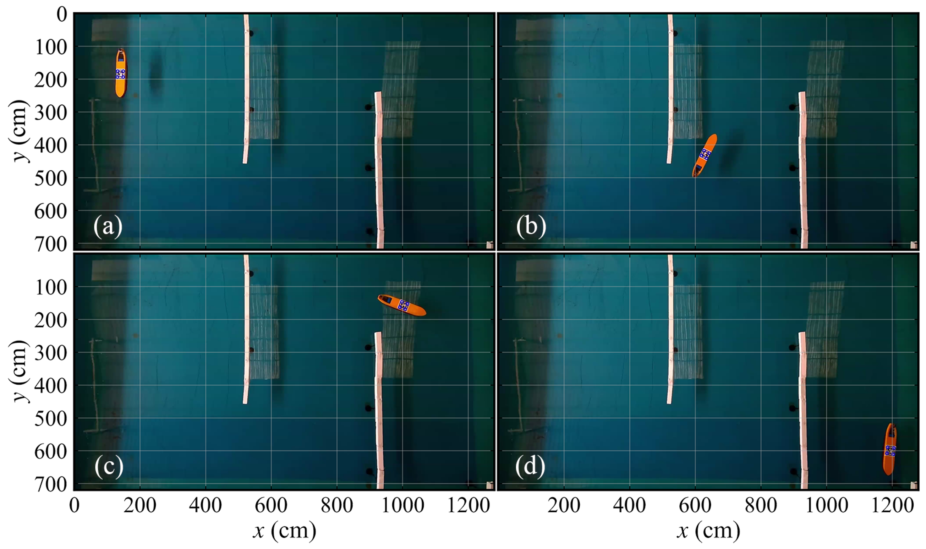
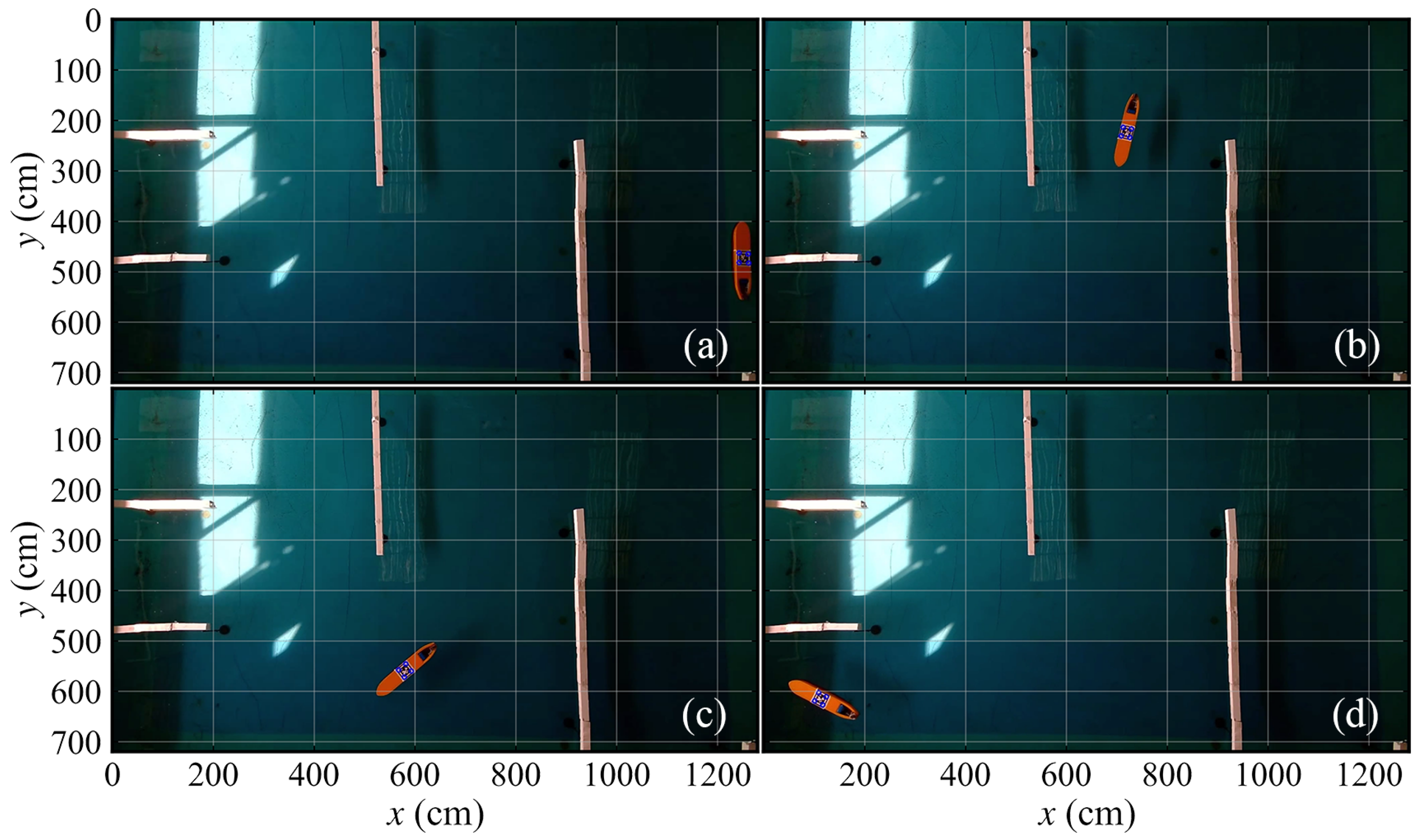
Figure 19 provides the overview of the two model test maps in a pool. In each map, we perform two model tests with different starting points and target points. At the beginning of each test, a series of guiding points are pre-determined, and the vessel is required to navigate along these points, with the propeller’s PWM set to 80. Taking test 1-2 and test 2-1 as examples, Figure 20 and Figure 21 separately present crucial navigation snapshots. In Figure 20a, the ASV just starts its navigation, in Figure 20b,c, it successfully avoids obstacles around the bend, and in Figure 20d, the ASV reaches its target point. In addition, the ASV is in the initial navigation stage in Figure 21a, and in Figure 21b, it bypasses the obstacle. Then, the ASV gradually approaches its destination and achieves the destination, as shown in Figure 21d.

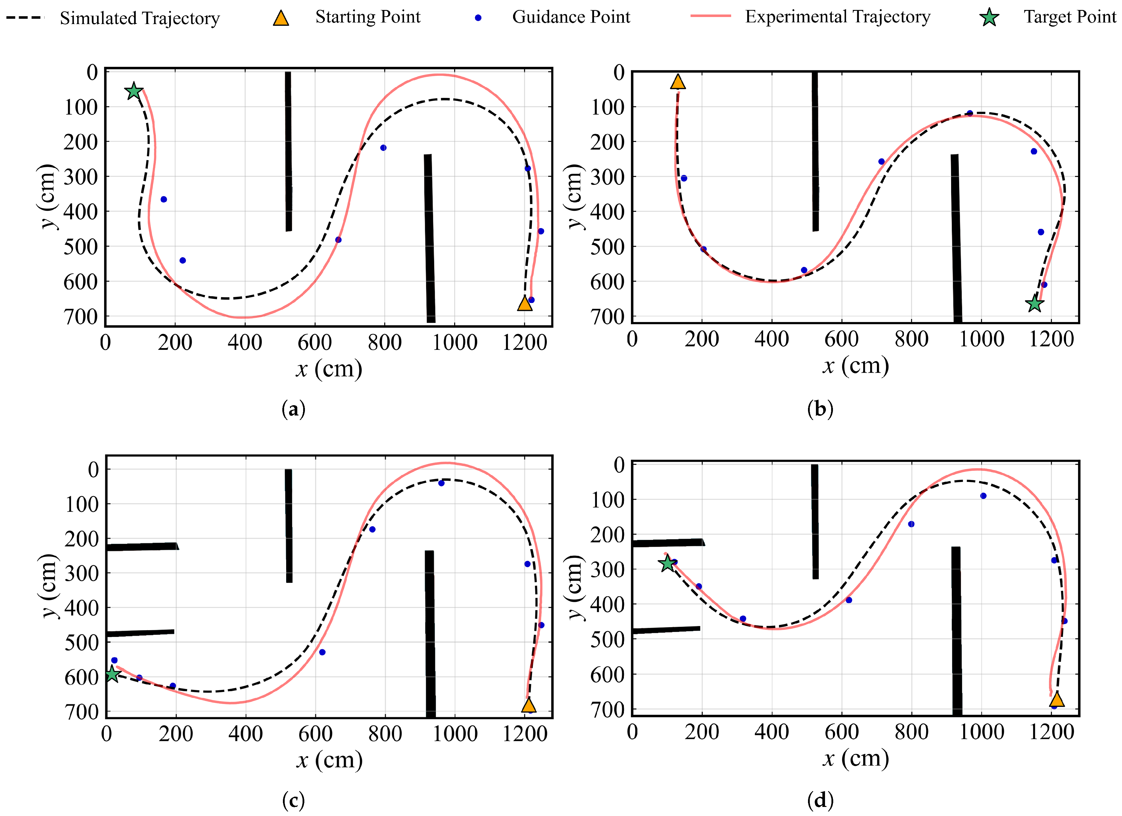
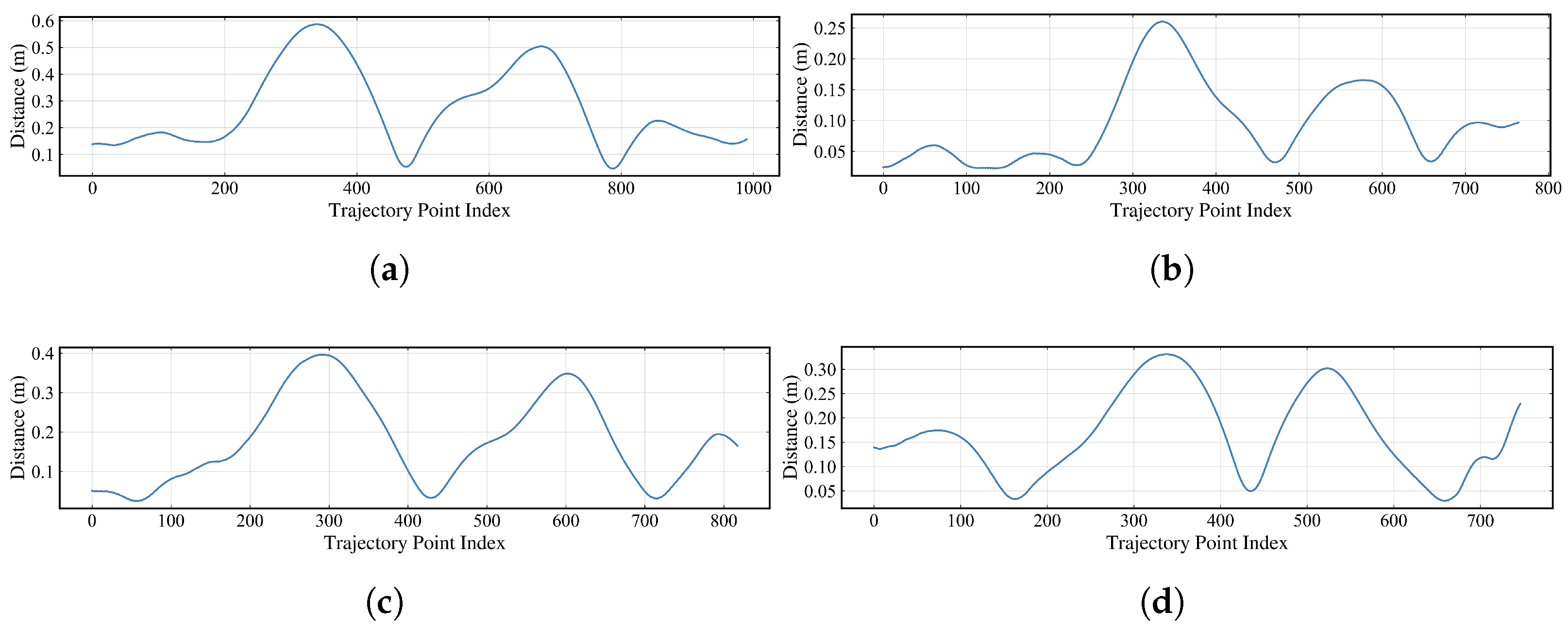
Comparisons between the experimental trajectory and the simulated trajectory in each test are shown in Figure 22. The red line denotes the experimental trajectory, while the black dot line is the simulated trajectory. It can be seen that there are deviations between the trajectories, mainly due to the limited scale of the pool, which restricts the turning space for the vessel. Thus, the guiding points only function to provide the desired course. Figure 23 demonstrates the changes in the deviation value, and

Table 5. The trajectory deviation values for each model test.

Test	Average Error (m)	Maximum Error (m)	Actual Trajectory Index of Maximum Error
1-1	0.270	0.587	340
1-2	0.096	0.260	336
2-1	0.178	0.396	291
2-2	0.165	0.331	338

illustrates the average and maximum distance error for each test. The results indicate that the average and maximum values are less than 0.3 m and 0.6 m, respectively. Notably, the maximum trajectory deviation occurs in test 1-1, which is 0.587 m at the point index of 340.

5.3.3. Collision Avoidance in Stochastic Environments

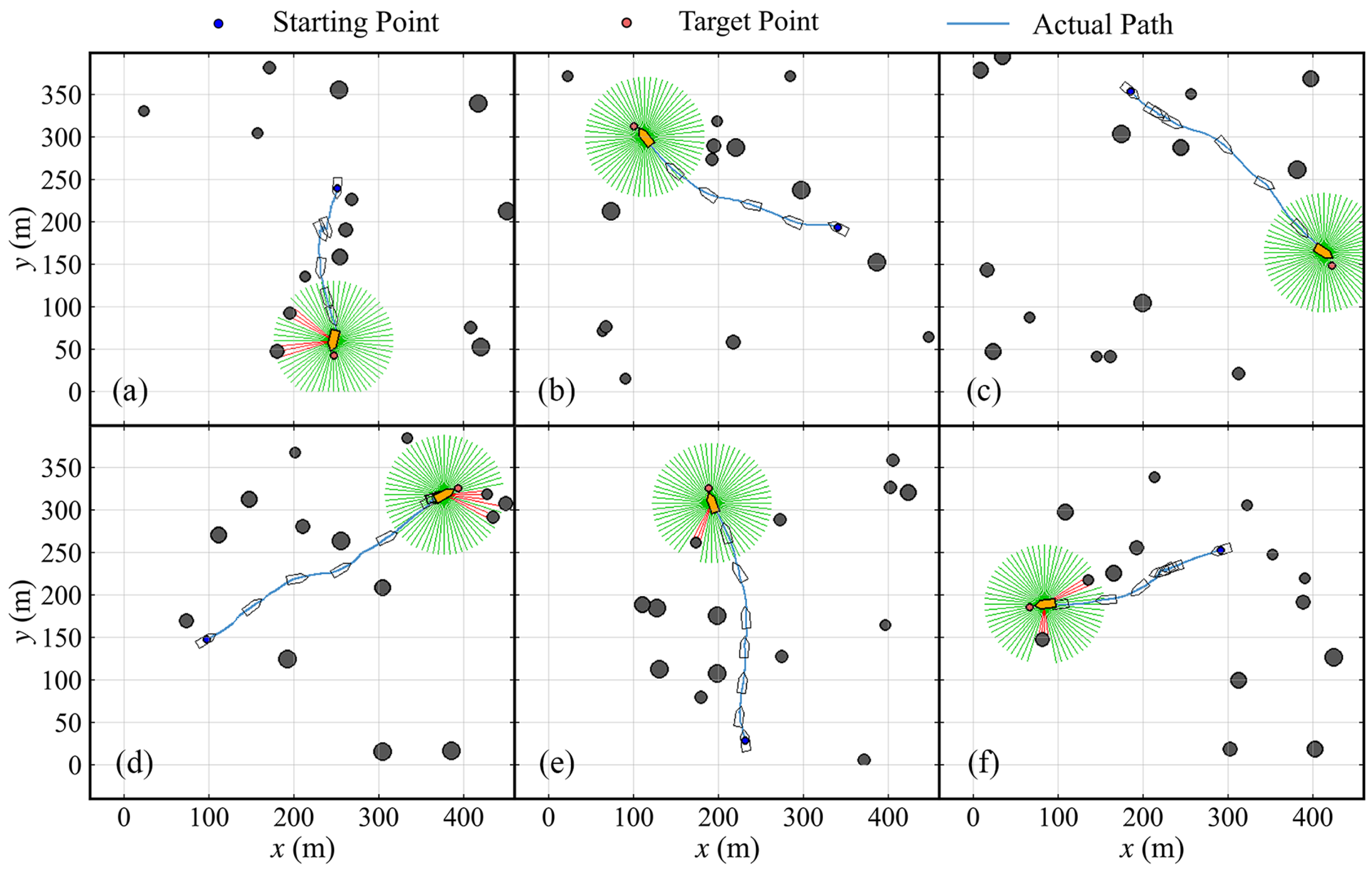
Simulation experiments, focused on the collision avoidance policy in environments characterized by random static and multiple dynamic obstacles, are conducted in this section. First, Figure 24 shows six simulation trajectory results of static obstacle avoidance experiments in calm water. The size of the simulation map is 640 m × 360 m, and the initial yaw angle of the ASV, radius range of the obstacle, detection radius of the LiDAR, and the number of laser beams are the same as those in Section 5.2.2. It is evident that, at various coordinate positions, the vessel effectively detects static obstacles and successfully achieves autonomous collision avoidance.

In Figure 25, the collision avoidance tasks are conducted in calm water, and the ASV encounters a single dynamic obstacle in situations of head on, crossing 1, crossing 2, and overtaking separately. The position of the ASV and the obstacle is recorded per 150 s. Figure 26a shows the change in the distance between the ASV and each dynamic obstacle. The specific minimum distance values are presented in

Table 6. The minimum distances between the ASV and obstacles in different encounter scenarios.

Encounter Scenario	Minimum Distance (m)	Time (s)
Head on	40.658	488.0
Crossing 1	42.769	285.0
Crossing 2	55.493	342.0
Overtaking	47.239	645.5

, and all of the minimum distances are above 40 m.

Figure 27 illustrates the schematic representations of the ASV successfully avoiding four dynamic obstacles under the environmental disturbances. Figure 26b presents the variation in distance between the vessel and obstacles over time, with the minimum distances detailed in

Table 7. The minimum distances between the ASV and obstacles in multiple dynamic obstacles scenario.

Obstacle Index	Minimum Distance (m)	Time (s)
No.1	56.869	722.5
No.2	59.884	727.0
No.3	58.246	480.0
No.4	22.741	839.5

. The initial position of the vessel is (140 m, 80 m), and the destination is set at (370 m, 300 m). The data indicate, that prior to 250 s, the vessel proceeds directly towards its target. At 400 s, with the virtual obstacles detected, the vessel sightly changes its heading. By 500 s, predictions were made for the trajectories of obstacles No.2 and No.3, and the ship maneuvers to avoid the imagined obstacles, finally bypassing No.2 and No.3 at 550 s. Then, the ship encounters obstacle No.4, and it preemptively maneuvers to avoid the predicted trajectory of the obstacle, navigating to the right side of No.4, while approaching the target point. At 839.5 s, the vessel reaches its closest proximity to the No.4 obstacle.

5.3.4. Autonomous Navigation and Collision Avoidance in Complex Environment

This section presents simulations of hybrid ship autonomous navigation and collision avoidance in complex environments. The navigation commences at the coordinates (465 m, 634 m) and terminates at (905 m, 514 m). Upon detection of obstacles by the LiDAR system (excluding virtual obstacles), the distance ${\Delta }_2$ is employed to adjust the local target point. In other cases, the looking forward distance is set to ${\Delta }_1$. The environmental conditions are consistent with those detailed in Table 3.

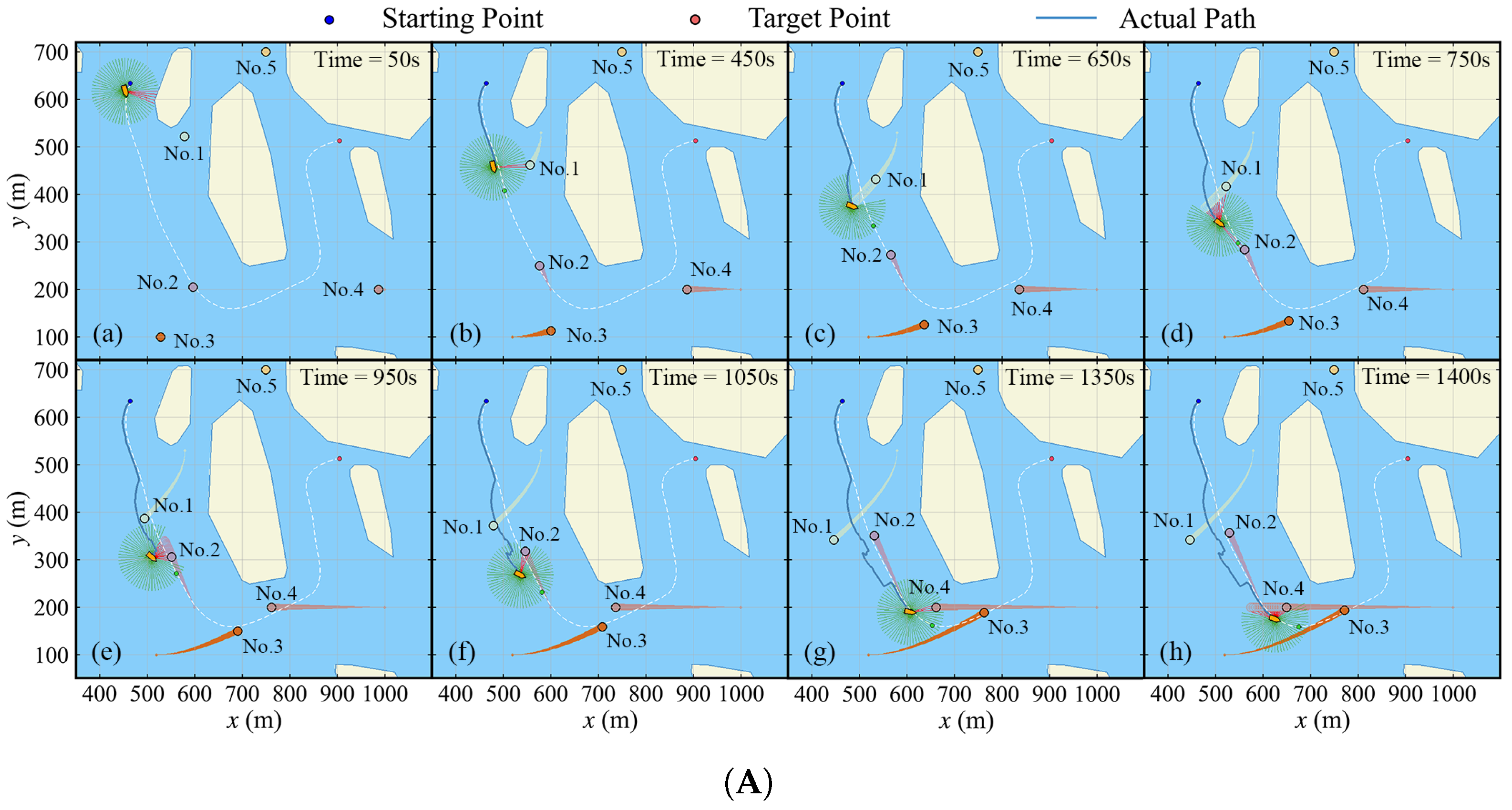
Figure 28 shows the simulation results at each specific time step. Figure 29 provides data regarding the distances between the ASV and other obstacles, the distance between the ASV actual path and global path, and the rudder angle and propeller PWM over time. The minimum distances can be found in

Table 8. The minimum distances between the ASV and dynamic obstacles in complicated water.

Obstacle Index	Minimum Distance (m)	Time (s)
No.1	76.321	665.0
No.2	37.078	989.5
No.3	56.530	2041.0
No.4	30.866	1421.0
No.5	25.081	2650.0

. At the beginning, a global path avoiding static obstacles is provided. Prior to 450 s, the vessel executes the path-following mode with a constant propeller PWM. Due to environmental disturbances, there is a stable path error around 5 m. After 450 s, the vessel turns right to avoid No.1, thus completing the crossing in front of No.1 eventually. At 665 s, the minimum distance between the two is 76.321 m. Later, at 750 s, the vessel encounters obstacle No.2. The vessel also turns right to avoid it, with the minimum distance at 989.5 s being 37.078 m, and successfully avoids No.2 after 1050 s. At 1350 s, the vessel is positioned directly in front of obstacle No.4. At this time, the ASV continues its forward navigation, passing directly in front of No.4, with the minimum distance to No.4 being 30.866 m. After 1950 s, the vessel is situated behind obstacle No.3, and at 2100 s, it passes between the static obstacle and No.3, subsequently switching to the path-following mode and gradually approaching No.5. At 2550 s, the vessel executes a right turn to avoid an impending obstacle. At 2650 s, the distance between the two is 25.081 m. Finally, at 2806.5 s, the vessel successfully arrives at the target point.

6. Conclusions

In this paper, we take an under-actuated VLCC ship model as the research subject. Utilizing the SAC algorithm, a navigation behavior control system that is suitable for a complex marine environment is proposed, enabling the vessel to autonomously follow pre-defined paths and avoid obstacles. To address the challenge of avoiding dynamic obstacles, a trajectory prediction algorithm that combines KF and LSTM is introduced. When the vessel identifies a potential collision risk using the CPA criteria, it then predicts the future trajectory of dynamic obstacles based on their historical coordinate data and considers the points on the predicted trajectory as virtual obstacles to avoid, thus taking collision avoidance measures in advance. Throughout the training process of the path-following policy, the success rate consistently remains at $100\%$ after 50 epochs. For the collision avoidance policy, its success rate stabilizes between $90\%$ and $100\%$. By performing numerical simulation tests and building prototype system for the ship model, the path-following policy is validated in different navigation environments. Additionally, through numerical simulations, successful autonomous navigation and collision avoidance tests are also completed with static unknown obstacles, a single dynamic obstacle in different encounter scenarios, multiple dynamic obstacles, and in complex environments.

However, considering the practical use of the DRL-based autonomous navigation, the following research could be carried out in future work:

• The real-world conditions may degrade sensor performance. Future work will first integrate multi-sensor fusion and noise-adaptive perception modules to enhance robustness, building on the model-agnostic advantages of the current framework.
• While this work demonstrates the efficacy of the proposed hybrid framework for underactuated ASV path following and collision avoidance, comprehensive comparisons with traditional methods or other DRL algorithms are left to future studies, as they require tailored adaptations to partial observability and actuator constraints.
• This study assumes dynamic obstacles follow predefined trajectories, excluding reciprocal interactions. Future work will integrate game-theoretic, COLREGS, and MARL frameworks to model adaptive multi-agent behaviors, critical for crowded waterways.

References

1. Yan, X.; Wang, S.; Ma, F. Review and prospect for intelligent cargo ships. Chin. J. Ship Res. 2021, 16, 1–6. [Google Scholar] [CrossRef]
2. Zubowicz, T.; Armiński, K.; Witkowska, A.; Śmierzchalski, R. Marine autonomous surface ship-control system configuration. IFAC-PapersOnLine 2019, 52, 409–415. [Google Scholar] [CrossRef]
3. de Vos, J.; Hekkenberg, R.G.; Banda, O.A.V. The Impact of Autonomous Ships on Safety at Sea—A Statistical Analysis. Reliab. Eng. Syst. Saf. 2021, 210, 107558. [Google Scholar] [CrossRef]
4. Azar, A.T.; Koubaa, A.; Ali Mohamed, N.; Ibrahim, H.A.; Ibrahim, Z.F.; Kazim, M.; Ammar, A.; Benjdira, B.; Khamis, A.M.; Hameed, I.A.; et al. Drone Deep Reinforcement Learning: A Review. Electronics 2021, 10, 999. [Google Scholar] [CrossRef]
5. Irshayyid, A.; Chen, J.; Xiong, G. A review on reinforcement learning-based highway autonomous vehicle control. Green Energy Intell. Transp. 2024, 3, 100156. [Google Scholar] [CrossRef]
6. Lokukaluge, P.; Joao, C.; Carlos, G.S. Fuzzy logic based decision making system for collision avoidance of ocean navigation under critical collision conditions. J. Mar. Sci. Technol. 2011, 16, 84–99. [Google Scholar] [CrossRef]
7. Campbell, S.; Naeem, W. A Rule-based Heuristic Method for COLREGS-compliant Collision Avoidance for an Unmanned Surface Vehicle. IFAC Proc. Vol. 2012, 45, 386–391. [Google Scholar] [CrossRef]
8. Wu, B.; Cheng, T.; Yip, T.L.; Wang, Y. Fuzzy logic based dynamic decision-making system for intelligent navigation strategy within inland traffic separation schemes. Ocean. Eng. 2020, 197, 106909. [Google Scholar] [CrossRef]
9. Fan, Y.; Sun, X.; Wang, G. An autonomous dynamic collision avoidance control method for unmanned surface vehicle in unknown ocean environment. Int. J. Adv. Robot. Syst. 2019, 16, 1729881419831581. [Google Scholar] [CrossRef]
10. Jawhar, G.; Lamia, I.; Maarouf, S. Adaptive Finite Time Path-Following Control of Underactuated Surface Vehicle with Collision Avoidance. J. Dyn. Syst. Meas. Control 2019, 141, 121008. [Google Scholar] [CrossRef]
11. Ge, Y.; Zhong, L.; Qiang, Z.J. Research on USV Heading Control Method Based on Kalman Filter Sliding Mode Control. In Proceedings of the 2020 Chinese Control and Decision Conference (CCDC), Hefei, China, 22–24 August 2020; pp. 1547–1551. [Google Scholar] [CrossRef]
12. Surjeet, B.; Nishu, G.; Ahmed, A.; Isha, B.; Rami, M.; Sarmad, M.; Firas, A. A survey on deep reinforcement learning architectures, applications and emerging trends. IET Commun. 2022, 19, e12447. [Google Scholar] [CrossRef]
13. Zhao, L.; Myung-Il, R.; Lee, S. Control method for path following and collision avoidance of autonomous ship based on deep reinforcement learning. J. Mar. Sci. Technol. 2019, 27, 1. [Google Scholar]
14. Mohammad, E.; Nader, Z.; Mahtab, S.; Amilcar, S.; Bruno, B.M.; Stan, M. Using Deep Reinforcement Learning Methods for Autonomous Vessels in 2D Environments. In Advances in Artificial Intelligence; Springer: Cham, Switzerland, 2020; pp. 220–231. [Google Scholar]
15. Wu, X.; Chen, H.; Chen, C.; Zhong, M.; Xie, S.; Guo, Y.; Fujita, H. The autonomous navigation and obstacle avoidance for USVs with ANOA deep reinforcement learning method. Knowl.-Based Syst. 2020, 196, 105201. [Google Scholar] [CrossRef]
16. Yan, N.; Huang, S.; Kong, C. Reinforcement Learning-Based Autonomous Navigation and Obstacle Avoidance for USVs under Partially Observable Conditions. Math. Probl. Eng. 2021, 2021, 5519033. [Google Scholar] [CrossRef]
17. Zhou, C.; Wang, Y.; Wang, L.; He, H. Obstacle avoidance strategy for an autonomous surface vessel based on modified deep deterministic policy gradient. Ocean. Eng. 2022, 243, 110166. [Google Scholar] [CrossRef]
18. Gao, M.; Kang, Z.; Zhang, A.; Liu, J.; Zhao, F. MASS autonomous navigation system based on AIS big data with dueling deep Q networks prioritized replay reinforcement learning. Ocean. Eng. 2022, 249, 110834. [Google Scholar] [CrossRef]
19. Yang, X.; Han, Q. Improved reinforcement learning for collision-free local path planning of dynamic obstacle. Ocean. Eng. 2023, 283, 115040. [Google Scholar] [CrossRef]
20. Fossen, T.I. Handbook of Marine Craft Hydrodynamics and Motion Control; Wiley: Hoboken, NJ, USA, 2021. [Google Scholar] [CrossRef]
21. Skjetne, R.; Smogeli, Ø.; Fossen, T.I. Modeling, identification, and adaptive maneuvering of CyberShip II: A complete design with experiments. IFAC Proc. Vol. 2004, 37, 203–208. [Google Scholar] [CrossRef]
22. Wang, X.; Wang, S.; Liang, X.; Zhao, D.; Huang, J.; Xu, X.; Dai, B.; Miao, Q. Deep Reinforcement Learning: A Survey. IEEE Trans. Neural Netw. Learn. Syst. 2022, 35, 5064–5078. [Google Scholar] [CrossRef]
23. Sutton, R.; Barto, A. Reinforcement Learning: An Introduction. IEEE Trans. Neural Netw. 1998, 9, 1054. [Google Scholar] [CrossRef]
24. Chen, W.; Qiu, X.; Cai, T.; Dai, H.; Zheng, Z.; Zhang, Y. Deep Reinforcement Learning for Internet of Things: A Comprehensive Survey. IEEE Commun. Surv. Tutor. 2021, 23, 1659–1692. [Google Scholar] [CrossRef]
25. Zheng, Y. Research on Tracking Control of High-Speed Underacmated Unmanned Surface Vessels. Master’s Thesis, Harbin Engineering University, Harbin, China, 2021. [Google Scholar]
26. Liu, J. Research on Track Planning and Tracking Control Algorithm of Underactuated Ship. Master’s Thesis, Wuhan University of Technology, Wuhan, China, 2022. [Google Scholar]
27. Zhu, H.; Ding, Y. Optimized Dynamic Collision Avoidance Algorithm for USV Path Planning. Sensors 2023, 23, 4567. [Google Scholar] [CrossRef]
28. Haarnoja, T.; Zhou, A.; Abbeel, P.; Levine, S. Soft Actor-Critic: Off-Policy Maximum Entropy Deep Reinforcement Learning with a Stochastic Actor. arXiv 2018, arXiv:1801.01290. [Google Scholar]
29. Sepp, H.; Jürgen, S. Long Short-term Memory. Neural Comput. 1997, 9, 1735–1780. [Google Scholar] [CrossRef]
30. Welch, G.; Bishop, G. An Introduction to the Kalman Filter; University of North Carolina at Chapel Hill: Chapel Hill, NC, USA, 1994. [Google Scholar]
31. Mercat, J.; Zoghby, N.E.; Sandou, G.; Beauvois, D.; Gil, G.P. Kinematic Single Vehicle Trajectory Prediction Baselines and Applications with the NGSIM Dataset. arXiv 2020, arXiv:1908.11472. [Google Scholar] [CrossRef]
32. Stenersen, T.C. Guidance System for Autonomous Surface Vehicles. Master’s Thesis, NTNU, Trondheim, Norway, 2015. [Google Scholar]
33. Duong, N.; Ronan, F. A Transformer Network with Sparse Augmented Data Representation and Cross Entropy Loss for AIS-Based Vessel Trajectory Prediction. IEEE Access 2024, 12, 21596–21609. [Google Scholar] [CrossRef]
34. Journee, J.; Massie, W. Offshore Hydromechanics, 1st ed.; Delft University of Technology, Faculteit Civiele Techniek en Geowetenschappen: Delft, The Netherlands, 2000. [Google Scholar]
35. Daidola, J.; Graham, D.; Chandrash, L. A simulation program for vessel’s maneuvering at slow speeds. In Proceedings of the 11th Ship Technology and Research Symposium (STAR), Portland, OR, USA, 21–23 May 1986. [Google Scholar]
36. Shen, X.; Wang, C.; Lian, S.; Li, S. Wind waVe spectrum estimation of small generating area by the maximum entropy method. J. Chang. Univ. Sci. Technol. (Nat. Sci.) 2007, 4, 39–43. [Google Scholar]
Figure 1. The reference coordinate systems. (a) The Earth and body-fixed coordinate systems in the six-DOF scenario. The original point O is located at the mass center of the ship. (b) The three-DOF horizontal Earth and body-fixed coordinate systems.
Jmse 13 02108 g001
Figure 2. The general view of the path-following task in three-DOF horizontal plane, which is based on course tracking control.
Jmse 13 02108 g002
Figure 3. The schematic views of LiDAR on ASV. (a) A LiDAR on an ASV is emitting laser beams in two-dimensional space. (b) The weight distribution of LiDAR laser beams. The beams located in front of the ASV possess a higher weight value showing a higher collision risk, whereas those directed backwards hold a lower weight value of collision risk.
Jmse 13 02108 g003
Figure 4. In the structure of the LSTM unit, c represents the memory cell’s stored value, h denotes the output value of the LSTM, and x is the input value from the user. The LSTM unit has four inputs and one output. The inputs consist of the vector x t 1 , h t 1 , c t 1 along with the activation signals for the forget gate f t , the input gate i t , and the output gate o t .
Jmse 13 02108 g004
Figure 5. The flowchart of the policy training process. If the current iterative step is larger than the policy training start step, the model training commences.
Jmse 13 02108 g005
Figure 6. The points in the predicted trajectory are considered as virtual obstacles that the ASV needs to avoid.
Jmse 13 02108 g006
Figure 7. The flowchart of the hybrid system, where P t a r g e t represents the coordinates of the final target point. Δ is the distance threshold.
Jmse 13 02108 g007
Figure 8. The schematic view of CPA, where U A and U B are the resultant velocities.
Jmse 13 02108 g008
Figure 9. Visualization of the path-following policy training process in different training stages. The epoch of each sub-figure (ac) is 1, 20, and 175, respectively.
Jmse 13 02108 g009
Figure 10. The training results of the path-following policy. (a) Success rate per epoch. (b) Average return and standard deviation per step in each epoch.
Jmse 13 02108 g010
Figure 11. Visualization of the collision avoidance policy training process in different training stages. The epoch of each sub-figure (ac) is 1, 25, and 300, respectively.
Jmse 13 02108 g011
Figure 12. The training results of the collision avoidance policy. (a) Success rate per epoch. (b) Average return and standard deviation per step in each epoch.
Jmse 13 02108 g012
Figure 13. Visualization of the AIS trajectory data.
Jmse 13 02108 g013
Figure 14. MSE loss of KF-LSTM trajectory predictor. (a) Average training loss in each epoch. (b) Average validation loss in each epoch.
Jmse 13 02108 g014
Figure 15. Wind load coefficients of the ASV in different headings. (a) C x w i n d . (b) C y w i n d . (c) C z w i n d .
Jmse 13 02108 g015
Figure 16. Path-following task results in different scenarios. (a) Simulation results in static water. (b) Simulation results in water with external disturbances.
Jmse 13 02108 g016
Figure 17. Time domain curves of yaw angle, path-following error, and rudder angle in scenarios I and II . (a) Yaw angle (Scenario I ). (b) Yaw angle (Scenario II ). (c) Path-following error (Scenario I ). (d) Path following error (Scenario II ). (e) Rudder angle (Scenario I ). (f) Rudder angle (Scenario II ).
Jmse 13 02108 g017
Figure 18. The automatic behavior system of the under-actuated ASV state calculator.
Jmse 13 02108 g018
Figure 19. The overview of two maps for model tests. (a) The map for test 1-1 and 1-2. (b) The map for test 2-1 and 2-2.
Jmse 13 02108 g019
Figure 20. Crucial navigation snapshots of test 1-2 in map 1. (a) Initial status. (b) During the navigation. (c) During the navigation. (d) Final stage.
Jmse 13 02108 g020
Figure 21. Crucial navigation snapshots of test 2-1 in map 2. (a) Initial status. (b) During the navigation. (c) During the navigation. (d) Final stage.
Jmse 13 02108 g021
Figure 22. Comparisons between experimental trajectory and simulated trajectory. (a) Test 1-1. (b) Test 1-2. (c) Test 2-1. (d) Test 2-2.
Jmse 13 02108 g022
Figure 23. Distance errors between experimental trajectory and simulated trajectory. The x-axis denotes the index of experimental trajectory points. (a) Test 1-1. (b) Test 1-2. (c) Test 2-1. (d) Test 2-2.
Jmse 13 02108 g023
Figure 24. Trajectories of the ASV in autonomous collision avoidance tasks. (a) Task 1. (b) Task 2. (c) Task 3. (d) Task 4. (e) Task 5. (f) Task 6.
Jmse 13 02108 g024
Figure 25. The schematic representations of the ASV successfully avoiding four dynamic obstacles in calm water. (a) Task 1. (b) Task 2. (c) Task 3. (d) Task 4.
Jmse 13 02108 g025
Figure 26. The variation in distance between the vessel and obstacles. (a) Single dynamic obstacle in different encounter scenarios. (b) Multiple dynamic obstacles scenario.
Jmse 13 02108 g026
Figure 27. The schematic representations of the ASV successfully avoiding four dynamic obstacles under environmental disturbances.
Jmse 13 02108 g027
Figure 28. The general views of the ASV navigating in a complex environment. (A) The navigation between 50 s and 1400 s. (B) The navigation between 1550 s and terminal time step.
Jmse 13 02108 g028aJmse 13 02108 g028b
Figure 29. The variation in distance between the ASV and the obstacles and the motion parameters change in a complicated environment. (a) The variation in distance between the ASV and dynamic obstacles. (b) The distance between ship actual path and global path. (c) Rudder angle. (d) Propeller PWM.
Jmse 13 02108 g029