Article

Exploring Time-Series Deep Learning Models for Ship Fuel Consumption Prediction

1
College of Information Engineering, Shanghai Maritime University, Shanghai 201306, China
2
Merchant Marine College, Shanghai Maritime University, Shanghai 201306, China
*
Author to whom correspondence should be addressed.
J. Mar. Sci. Eng. 2025, 13(11), 2102; https://doi.org/10.3390/jmse13112102
Submission received: 30 September 2025 / Revised: 22 October 2025 / Accepted: 29 October 2025 / Published: 4 November 2025

Abstract

The fuel consumption of ships is an important component of shipping operation costs and also a significant source of greenhouse gas emissions. Accurate fuel consumption prediction is of great significance for optimizing the energy efficiency management of ships, reducing operating costs, and minimizing environmental pollution. In addition, we have also observed that the fuel consumption data of ships usually have a strong temporal correlation. Therefore, in order to study whether the time-series factors of ship fuel data are helpful for SFC prediction and the performance of various deep learning models in ship fuel consumption prediction, this paper proposes three classes of models for comparative study: RNN-based models, attention-based models such as Transformer and Informer, which are applied to the field of ship fuel consumption for the first time, and RNN–attention mixed models. The experimental results show that there is indeed a lag in ship navigation data, and the processing of time-series data is of great significance for fuel consumption prediction. Moreover, we have found that on real ship operation datasets, Informer is the best-performing model with 1.46 and 0.969 for MSE and R 2 scores. The prediction performance of Informer is significantly better than that of other methods, which provides a new direction for future ship fuel consumption prediction.

1. Introduction

Shipping plays a paramount role in global transportation [1]. With a substantial shipping tonnage, effective management of ship fuel consumption (SFC) holds significant sway over operating costs for shipping companies [2] and global carbon dioxide emissions [3]. Additionally, starting from 1 January 2023, ships with a gross tonnage of 5000 or more, and those complying with the Energy Efficiency Design Index (EEDI), are mandated to annually report their Carbon Intensity Indicator (CII) and CII rating. Vessels rated D for three consecutive years or E for one year are required to submit corrective action plans outlining measures to attain a C or higher index [4]. This regulation compels shipping firms to adopt strategies for energy conservation and carbon emission reduction.
For already operational ships, retrofitting main engines with cleaner fuels (such as methanol or LNG) or modifying hulls might not be feasible or convenient. In such cases, effective SFC management becomes an ideal solution [5], achieved through real-time SFC monitoring during voyages and optimization of ship speeds. Accurate SFC prediction models offer a viable approach to manage and curtail SFC. Precise SFC prediction allows crews to monitor fuel consumption, receive alerts about anomalies, and optimize ship speeds to meet SFC or carbon emission targets.
Many machine learning methods have also been applied to SFC prediction and achieved certain results, such as Random Forest [5,6,7,8,9,10], XGBoost [1], and so on. Numerous domestic and international scholars have conducted extensive research on ship fuel consumption modeling. They analyze and summarize the experience of ship navigation and make predictions by combining machine learning models. Or, by using the numerous features of ships to create linear regression models for prediction, very good results have been achieved [11,12,13,14,15,16].
Although these algorithms have been proven effective in predicting fuel consumption parameters, most existing models mainly consider external meteorological conditions and internal thermal parameters as inputs. However, we found that the fuel consumption data of ships has a strong temporal correlation. The fuel consumption of a ship is not only related to its current state but often also to its historical state. Furthermore, the operating status, environmental conditions, and operation modes of ships all change over time. If we can capture these dynamic changes, the prediction results may be more accurate. Therefore, we attempt to use a time-series analysis model to solve the problem of ship fuel consumption prediction.
Notably, algorithms such as artificial neural networks (ANNs) [17,18,19,20,21,22,23], long short-term memory (LSTM) [24,25,26], and bidirectional LSTM (BiLSTM) [27,28] have been evaluated, showing relatively high prediction accuracy. In particular, LSTM-based models have shown outstanding effectiveness compared to other models due to the ability to capture complex patterns in data and the time-series nature of SFC data. In recent years, except for LSTM-based time-series deep learning models, attention-based deep learning models like Transformer have received much attention in many domains, such as in finance, energy management, transportation, and logistics [29,30]. However, their exploration in SFC prediction remains limited. The transformer model, which proposed the attention mechanism, has not been applied to the field of time-series prediction of ship fuel consumption. Therefore, this paper selects the Transformer, Transformer–No–Decoder, iTransformer, and Informer models for experiments to explore whether time-series prediction based on the attention mechanism is suitable for the field of ship fuel consumption prediction and whether it has good accuracy and generalization. At the same time, the mixed model combining BiLSTM and attention was applied to SFC prediction, which significantly improved the prediction accuracy [28]. Therefore, we combined LSTM, BiLSTM, and attention into a mixed model to test its robustness and accuracy for long-term ship fuel consumption sequences. All of our experiments and validations are based on ship fuel consumption data. All indicators are also calculated based on fuel consumption data and used for performance evaluation of all algorithms. The fuel consumption data of ships mainly consists of the fuel consumption of the main engine, which will be introduced in Section 5.
Therefore, our paper addresses a gap by thoroughly evaluating different time-series deep learning models in SFC predictions, which specifically speaking makes three main contributions:
  • We theoretically analyzed the possible effect factors of predicting SFC based on ship energy efficiency data, including the traditional propulsion power, resistance, and time-series dependency factors.
  • We implemented in total nine time-series deep learning models for the SFC prediction task, including three RNN-based time series models, four attention-based models, and two RNN–attention mixed models. Among them, we applied models such as Transformer, iTransformer, and Informer to the prediction of ship fuel consumption for the first time and discovered their significance in improving the prediction accuracy.
  • We also implemented the promising XGBoost as a representative of traditional machine learning methods for the SFC prediction task and then comprehensively compared the total ten machine learning models and evaluated their respective applicability and accuracy for SFC prediction.
The remainder of this paper is structured as follows: Section 2 introduces preliminary concepts. Section 3 outlines related work. Section 4 details the exploration of time-series deep learning models and the proposed hybrid deep learning model for SFC prediction, while Section 5 discusses our evaluation findings. Finally, Section 6 concludes our research, suggesting potential avenues for future deep learning-based SFC prediction studies.

2. Preliminaries

2.1. Problem Definition

In this section, we rigorously define the problem of SFC prediction based on time-series deep learning models, encompassing the journey from input data to the final evaluation outcomes.
Definition 1. 
Let S be a ship energy efficiency data source characterized by attributes ( A 1 , A 2 , , A n ) . We denote each record as r = ( r 1 , r 2 , , r n )     S , where r constitutes a tuple in conformity with the attribute schema of data source S. Attributes ( A 1 , A 2 , , A n ) represent a collection of properties related to the ship, encompassing essential aspects like the timestamp when the ship data was collected, ship speed, environmental conditions, and ship fuel consumption (SFC). t s represents the length of the time window, which is the length of the input matrix. The objective is to address the SFC single-step real-time prediction problem, which involves employing one or multiple machine learning algorithms on a subset of S (the order of the ship energy efficiency data is maintained) designated as training data, with a chosen set of attributes S as input features ( F 1 , F 2 , , F n ) and a time step value t s , forming an input matrix. The goal is, given the input matrix covering the i t h to i + t s time step, to establish a predictive model M capable of foreseeing the next SFC value at the i + t s + 1 time step, which manifests as output O. In other words, our SFC prediction problem is counted as a single-step, one-attribute prediction problem.
Note that the SFC-related output feature used in our research is the fuel consumption of the main engine, which is derived by dividing the disparity between the inflow and outflow of fuel in the main engine by the ship’s speed through the water, which is more meaningful for developing a fuel consumption model to guide ship operations based on the analysis of [1,18].

2.2. Evaluation Metrics

According to Section 2.1, the result of the SFC prediction task is the fuel consumption value, which is a continuous numerical value. Therefore, SFC prediction tasks can be classified as regression problems, typically assessed using metrics such as the mean square error, the root mean square error, the mean absolute error, the mean absolute percentage error, or R 2 scores [31,32,33]. The above-mentioned five metrics will be applied in our experiments to evaluate the performance of different strategies from different angles. In the following, they are elaborated and explained together with their specific equations. In the equations that follow, ‘n’ represents the size of the test data, y ^ i denotes the predicted value for the i-th data point, y i represents the corresponding true value, and y ¯ i signifies the average of all true values y ( 1 n ) .
  • The mean square error (MSE) refers to the expected value of the squared error or loss and is calculated using the following equation:
    M S E = i = 1 n ( y i y ^ i ) 2 n
  • The root mean square error (RMSE) is closely related to the previously mentioned MSE and is equal to the square root of the MSE. This property brings it back to the scale of the target variable and makes it easier to interpret and understand.
    R M S E = i = 1 n ( y i y ^ i ) 2 n
  • The mean absolute error (MAE) is the arithmetic average of the absolute errors and is calculated as follows:
    M A E = i = 1 n y i y ^ i n
  • Mean absolute percentage error (MAPE) refers to the average relative error between the predicted value and the true value, expressed as a percentage, and is calculated as follows:
    M A P E = i = 1 n y i y ^ i y i n
  • The R-square score ( R 2 score) pertains to the coefficient of determination. It quantifies the model’s capability to predict unseen data and is computed using the following equation:
    R 2 = 1 i = 1 n ( y i y ^ i ) 2 i = 1 n ( y i y i ¯ ) 2
Comparing the previous four metrics, MSE penalizes larger errors more than smaller errors, making it sensitive to large deviations. In contrast, MAE treats all errors equally regardless of their magnitude and is less sensitive to outliers. In other words, MAE may overlook outliers in the predicted values. When the true value is relatively close to 0, the performance of MAPE will be very poor. Against the current background of real-time prediction of ship fuel consumption, we expect that the prediction results will maintain a high level of accuracy, as any significant deviation will affect the ship’s navigation decisions. The R 2 score is a relative metric, rendering it suitable for comparing different models trained on the same dataset. A higher value indicates a better fit. Therefore, among these five metrics, MSE and R 2 is selected as the main evaluation metric.

3. Related Work

Predicting SFC is a critical problem for ship energy efficiency management. So far, there have been abundant methods proposed to solve the SFC prediction task. According to a survey in this area [34], these methods can be broadly categorized into three types: white-box theoretical models, black-box models, and gray-box models. White-box theoretical models (WBMs) are based on prior knowledge and deep insights into system physics, with known structures and parameters that offer strong interpretability [35]. WBMs can directly infer fuel consumption from ship line data and sea trial data [6]. Ships are affected by various factors during navigation. Analyzing the governing physical laws of WBMs is a relatively complex process. In extreme navigation environments, the actual prediction accuracy may be very low [36]. In contrast, black-box models (BBMs) are trained using machine learning techniques and rely on extensive real-time monitoring data. While these models can make accurate predictions without prior knowledge, they lack interpretability and extrapolation capability [37]. Meanwhile, BBMs also have the problems of overfitting and poor generalization ability. Due to the abundance of general factors in the SFC model, overfitting usually leads to low accuracy [38]. The poor generalization ability limits the application of the established SFC models in individual ships or specific situations [39]. To address these shortcomings, gray-box models have been introduced, combining the strengths of both white-box and black-box models. Gray-box models (GBMs) estimate parameters for physically based models using collected data or integrate black-box components into the model outputs [11,40]. Theoretically, the GBM is the combination of the WBM and BBM and performs better than a single model. The Gaussian process model, which is an example of a GBM, can be used to study fuel consumption [34]. The selection and application of these methods are crucial for improving the accuracy and reliability of ship fuel consumption predictions, especially in situations in which there is initially no available data that can be used to train an effective model for a new ship or one with newly-installed sensors. And we often need to train a new fuel consumption prediction model based on limited data for these new ships. Some researchers have also taken the time factor into account, analyzed the variation pattern of fuel consumption over time, and used GBMs to predict fuel consumption [41]. Their results were also very accurate.
The eXtreme Gradient Boosting (XGBoost) algorithm belongs to ensemble learning, which is a technique aimed at enhancing prediction performance by training multiple models instead of relying solely on a single model, combining predictions from diverse models to arrive at a final result [42]. It builds a strong predictive model by combining multiple weak learners, typically decision trees. The algorithm optimizes the model through an iterative process where each new tree corrects the residual errors of the previous trees [43]. XGBoost stands out as an efficient and robust machine learning algorithm suitable for various predictive modeling tasks. Its capability to handle large-scale data, incorporate regularization techniques, and perform well with imbalanced datasets makes it a preferred choice for researchers and practitioners. Given its flexibility and computational efficiency, XGBoost is an essential tool for predictive modeling in ship energy efficiency management and broader maritime applications [1].
With the increasing complexity of data and advancements in computing hardware, deep learning models are gaining attention as powerful predictive tools in the maritime industry. Known for their ability to learn complex data and sensitivity to implicit patterns or features in the data, deep learning models offer new possibilities for accurately predicting ship fuel consumption. By leveraging deep learning models, we can utilize latent correlations and non-linear features in large-scale data, thus enhancing prediction accuracy and robustness.
Among deep learning models, ANN-based models have been widely explored to predict SFC [17,18,19,20,21,22,23]. Kim et al. [18] demonstrated that artificial neural networks (ANNs) outperform multiple linear regression (MLR) models in prediction accuracy.
In addition to ANNs, long short-term memory (LSTM) networks are gaining attention due to their powerful self-learning capabilities and widespread application in processing and modeling maritime data [24,25,26]. Han et al. established a long short-term memory neural network model to predict the remaining lifespan of air filters and turbochargers in marine diesel engine systems [44]. The experimental results show that LSTM can predict the remaining service life of the machine under different load conditions relatively accurately. Liu et al. established a diesel engine exhaust temperature prediction model based on LSTM, which helps ships predict maintenance time earlier [45]. LSTM networks are particularly suited for handling time-series data of ships, capturing long-term dependencies and non-linear features. Thus, applying LSTM networks to ship fuel consumption prediction models is expected to improve prediction accuracy and stability.
BiLSTM has achieved excellent results in many sequence tasks. Park et al. utilized the bidirectional LSTM network as the main sequence model and introduced the Time Attention (TA) and Feature Attention (FA) mechanisms to capture time and feature importance, thereby achieving one-step fuel consumption prediction [46]. The more recent research [27,28] explored using BiLSTM for the SFC prediction problem and gained positive results. Specifically speaking, Chen et al. [27] considered both single-step and multiple-step SFC prediction and concluded that adopting BiLSTM for SFC prediction is a promising strategy. Meanwhile Zhang et al. improved the BiLSTM model structure by adding an attention layer, which is proven to be able to improve the SFC prediction accuracy [28].

4. Methodology

In this section, we introduce our exploration of predicting SFC using time-series deep learning models. The overall process using three categories of deep learning models is shown in Figure 1. In the following sections, we will elaborate on it from both data and model perspectives.

4.1. Ship Energy Efficiency Data

As sensor technology has developed, it has been widely applied to different domains, including the shipping industry in our research. Diversiform sensors have been installed on the ships, enabling the collection and utilization of sensor data for ship efficiency management. The attributes a ship energy efficiency dataset may contain vary a lot due to the sensors installed in different ships. The common sensors installed in a ship include sensors for detecting the ship main engine’s rotate speed and torque, sensors for detecting ship speed over ground and ship speed through water, sensors for recording the draft from the ship’s bow, stern, and left and right sides, sensors for collecting the external environmental conditions of a ship, such as the wind speed and direction and the wave height (data regarding the external environmental conditions of a ship can not only be collected by the sensors installed on the ship, but can also be added from a third-party data source. In our case, we only consider data directly collected from sensors), and sensors to record the ship’s latitude and longitude.

4.1.1. Characteristics of Ship Energy Efficiency Data

Different sensors might have different frequencies to collect data, However, commonly, based on the observation of our data so far, the entire ship energy efficiency dataset collects data every 10 to 15 s, appending each data record with a timestamp. Therefore, the dataset collected from the sensors can be called high-frequency time-series data and can comprise over two million records per year. Based on these extensive time-series datasets related to ship energy efficiency, SFC can be predicted accurately by using proper strategies.
From the point view of analyzing the effect factors for SFC prediction, based on the traditional methods that analyze the floating state and hydrodynamics, ship fuel is primarily consumed for propulsion power to drive the ship forward at a required sailing speed. Except for the propulsion power adopted by the ship, the ship resistance from the ship itself (such as the ship design and its loading condition) and the external environment such as the sea and the air is the other main factor that affects the SFC [34]. Therefore, among the attributes of ship energy efficiency data, those that are closely related to the ship’s propulsion (such as the main engine power) and resistance (such as ship draft, which reflects the loading condition of the vessel and wind speed and direction) have a very high correlation with the SFC. On one hand, the adopted prediction model should be able to capture the above-mentioned correlations based on the collected ship energy efficiency data to predict SFC. On the other hand, as introduced above, ship energy efficiency data belongs to the time-series data, and a pivotal characteristic of time-series data is the dependency among different data records. For ship energy efficiency data, if the dependency among different data records can be captured by certain models, this might lead to more accurate SFC prediction. The dependency can be reflected in the following aspects:
  • In cruising conditions, the adjacent data records have similar states, leading to similar SFCs as well.
  • Under changing circumstances, such as ship acceleration or deceleration, the SFC is a reflection of both the current state and the previous state. For instance, if the current speed through water is 12 knots, and the previous speed through water is higher or lower than 12 knots, i.e., the ship is accelerating or decelerating, the SFC values should not be the same.
  • Under some circumstances, the noise or outlier data record contained in the data can only be identified by analyzing multiple adjacent data records, which cannot be identified solely in the data itself.
  • As the frequency of ship energy efficiency data is relatively high, many changes occur gradually, including short-term subtle variations and long-term trends, with potential non-linear and lag effects between them.

4.1.2. Data Preparation for Modeling

Before training models for predicting SFC, the raw ship data collected from the sensors firstly needs to be cleaned to remove the abnormal data, which might bring negative effects for SFC prediction. Afterwards, based on all raw attributes that the ship energy efficiency data has, which attributes are selected as input features for training the SFC prediction model needs to be decided. Although, theoretically speaking, deep learning algorithms might be able to learn the best sets of features automatically during their learning progress [47], it is still preferred to directly provide known priori information as extended features to assist the training process. In our research, we made the following feature adaptions or extensions based on the collected raw ship energy efficiency data:
  • Based on the drafts recorded from the four sides of the ship, we calculated the average draft of the bow and astern draft and the difference between the bow and astern draft as trim. On one hand, the average draft reflects the loading conditions of ships; heavier loads lead to a deeper average draft, which requires more fuel to support the transportation of more goods. On the other hand, trim is another factor that has been proven to be able to influence ship fuel consumptions [48]. The draft difference of the ship’s left and right side is considered to have minor effects on SFC and can be neglected.
  • The ships’ slip ratio can be calculated to reflect the overall situation that a ship is currently in, since it indicates the theoretical and practical distance difference a ship can move forward when the propeller makes a turn.
This study adopts the sliding window method to divide the time window of the ship’s time-series data. Specifically, a fixed-length time window is used to slide over the time series, thereby converting continuous time-series data into a sample sequence suitable for input to machine learning models. We adopted the sliding window technology to select 150 pieces as the window length and divided the ship operation data with an original sampling frequency of 10 s into a continuous window of 25 min in length. Then the extended features can be added to the ship energy efficiency dataset to train the prediction model.

4.2. Predicting SFC Using Time-Series Deep Learning Models

As described in Section 4.1.1, the ship energy efficiency-related data belongs to time-series data and the data records are not independent of each other. In this circumstance, if algorithms are not able to capture certain dependencies among data records, the trained SFC prediction models will lose certain parts of information. Therefore, time-series deep learning models stand out for providing promising SFC prediction results due to their ability to capture temporal and global dependencies. So far, multiple time-series deep learing models have been proposed and applied to time-series data from different domains.
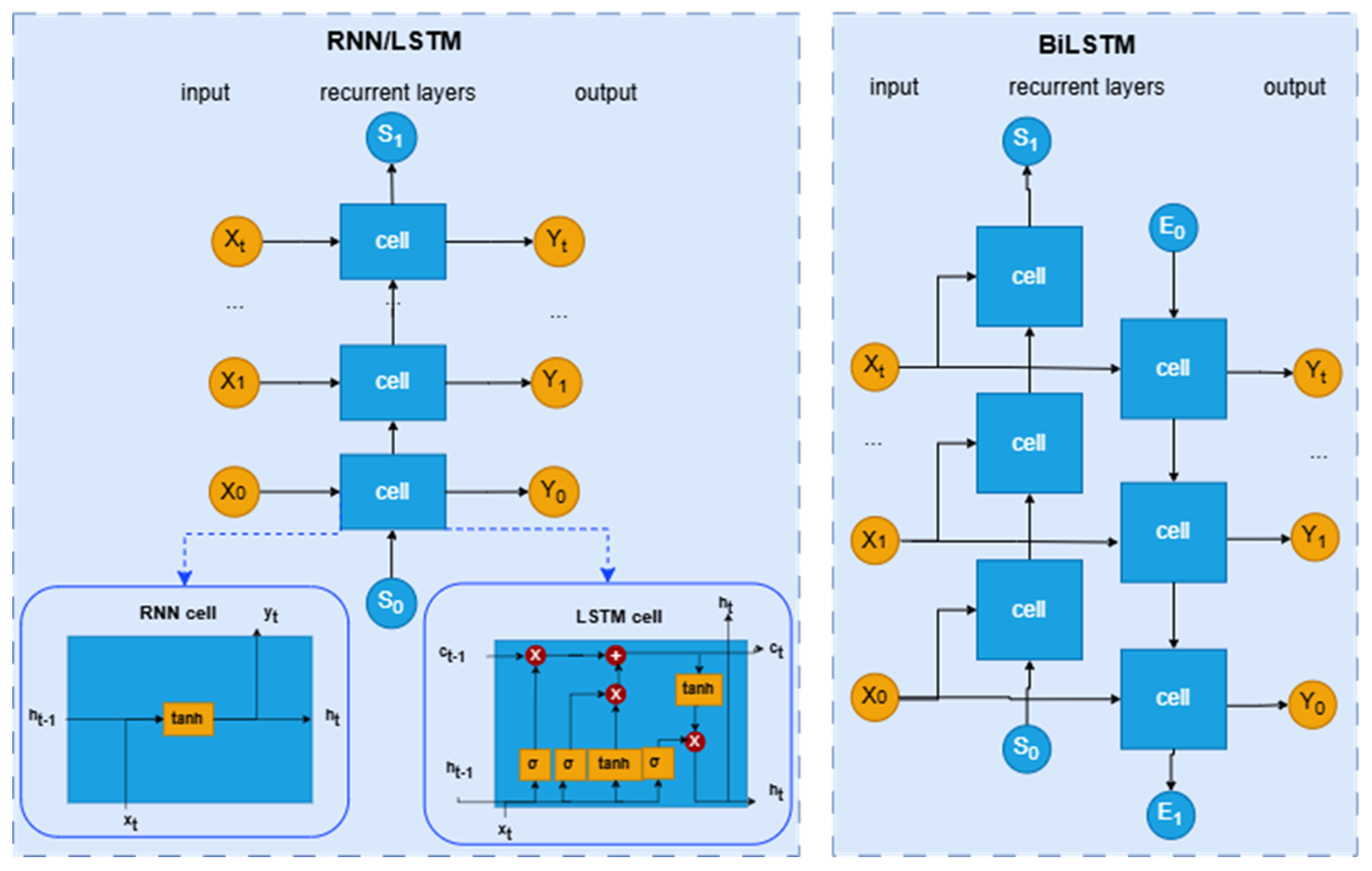
Among them, RNN-based models are inherently designed for time-series data. Recurrent Neural Networks (RNNs) are neural network structures with cyclic connections used for processing sequence data. Unlike traditional feedforward neural networks, RNNs can capture temporal correlations in sequences, but they suffer from issues like gradient vanishing and exploding. Basically, they operate by processing one time step at a time; each hidden state is updated based on the current input and the previous hidden state. This sequential recurrence explicitly encodes the temporal order and dependency, making them naturally suited to time-series data. In our research, we considered three RNN-based deep learning models: the original RNN, LSTM, and BiLSTM. Their structures are depicted in Figure 2. As we can see from it, the cell of the original RNN is relatively simple and accepts only the input of the current time step and the hidden state of the previous time step and updates the hidden state of this time step by a non-linear activation function, such as tanh, to generate the output for the current time step. The simplicity of RNN’s cells makes RNN lack the ability to memorize long-term dependency, leading to possible gradient vanishing and exploding [49].
To alleviate this problem, LSTM was proposed to capture both the long- and short-term dependency by adding memory cells and three gating mechanisms, the input gate, forget gate, and output gate [50], which allows LSTM to keep or drop information over longer periods. To conclude the structure of RNN and LSTM, they share a globally unidirectional structure of accepting new input at each time step, recurrently updating and outputting a new hidden state based on the information from previous time steps, while their differences are reflected in the specific process of updating the hidden state for the current time step. However, their unidirectional setting of processing time-series data from past to future limits their ability to capture complete dependencies, as there might be useful information in the backward direction as well, i.e., from future to past.
BiLSTM aims to solve the unidirectional problem of RNN and LSTM by adding another backward LSTM layer (shown in the right part of Figure 2), which makes it achieve better performance on tasks where context from both directions is valuable [51,52]. As RNN-based models are explicitly designed for time-series data, for predicting SFC, we can directly adopt and implement them without the need to modify the models’ structure.
The general structure of the original Transformer proposed by Vaswani et al. in 2017 is an encoder–decoder structure (see Figure 3a), where multiple encoders and decoders are stacked together. It captures dependencies by attention mechanisms instead of complex recurrences or convolutions used in RNN-based neural networks. In each encoder module, a multi-head attention layer is used to capture dependencies across different time steps, allowing the model to effectively learn the temporal evolution of specific fuel consumption (SFC) patterns over a given time range. This is followed by a feedforward layer to transform the learned representations non-linearly, enhancing feature extraction. In each decoder module, a masked multi-head attention layer ensures that predictions at each time step depend only on past observations, preventing information leakage during training. The multi-head attention layer then integrates the encoded features to refine contextual understanding. Subsequently, a feedforward layer processes the extracted features, and the final output passes through a linear layer followed by a softmax layer to generate the predicted fuel consumption values [53].
However, based on the observation from research in [54,55], the performance of the original Transformer with both encoder and decoder modules is limited by the cross-attention mechanism between the encoder and decoder. Therefore, in our research we adjusted the original Transformer with both an encoder and decoder by dropping the decoder module and output the encoded features directly to a fully connected layer to generate the predicted SFC results (as depicted in Figure 3b).
Subsequently, iTransformer was proposed [56]. The Transformer architecture was redesigned with the basic components remaining largely unchanged (see Figure 3c). Specifically, the time points of a single sequence are embedded into variable tokens, and the attention mechanism utilizes the variable tokens to capture multivariable correlations. Meanwhile, a feedforward network is applied to learn non-linear representations for each variable label.
Excepted for the above two Transformer-based models, under the category of attention-based deep learning models, we also implemented an Informer-based SFC prediction model. Informer is a novel Transformer-based model that effectively addresses the challenges of long-sequence time-series forecasting. By integrating innovative components such as ProbSparse self-attention, self-attention distilling, and a generative-style decoder, Informer significantly improves computational efficiency and scalability compared to traditional transformers. These enhancements enable it to capture long-range dependencies more accurately, making it a robust solution for a wide range of forecasting applications that require processing extended time-series data [57,58,59]. From a structural standpoint, the Informer model retains the encoder–decoder architecture of the original Transformer. However, it introduces several key enhancements to improve efficiency and performance (refer to Figure 3d) [60]. Firstly, it replaces the standard self-attention mechanism with a more efficient ProbSparse alternative. Secondly, it employs a technique of distilling attention results using convolutional and max-pooling layers to reduce their dimensionality. Finally, it proposes a generative-style decoder to mitigate the issue of cumulative errors during inference.
Figure 3. Comparison of attention-based model structures. (a) Transformer [53]. (b) Transformer–No–Decoder [53]. (c) iTransformer [56]. (d) Informer [60].
Jmse 13 02102 g003
The other series of models we considered in our research, which can also capture dependencies among different data records but implicitly capture the time-series dependency, are attention-based models (see Figure 4a). The attention mechanism captures dependencies among data records in a time-series dataset by computing pairwise interactions between all time steps. Each time step is represented by a feature vector, and the mechanism assigns a weight to every other time step based on the similarity between their representations. These weights determine how much each time step should contribute to the representation of the current step [53]. As we can see from the above-explained attention mechanism, the attention mechanism itself does not pay attention to the order of data records. Therefore, for attention-based models, to mitigate this problem, positional encoding is commonly added to the inputs to retain the order of the data records, as proposed in original self-attention-based model Transformer [53]. In traditional LSTM or BiLSTM, the hidden state at the last time step (or the concatenation of hidden states in two directions) is usually used to represent the entire sequence, which may lead to an information bottleneck because a fixed-dimensional vector may not be able to fully retain all the information in a long sequence. The attention mechanism constructs the context vector by weighted summing the hidden states of all time steps, thereby retaining more information. LSTM itself is already capable of handling long-sequence dependencies through gating mechanisms, but the attention mechanism can further assist the model in focusing on the parts of the sequence that are most relevant to the current output, thereby better capturing the key information in long sequences. BiLSTM captures past and future information through LSTM in both forward and backward directions, and the attention mechanism can weight the hidden states at different time steps based on the information in these two directions, thereby making more flexible use of the context (see Figure 4b).
Since the optimal time-series deep learning model option varies with the dataset and the application scenario, in our research, we explored applying the nine aforementioned time-series deep learing models, including RNN, LSTM, BiLSTM, the original Transformer, iTransformer, Transformer–No–Decoder, Informer, LSTM_Attention, and BiLSTM_Attention, to predict SFC and evaluated their respective performance.

5. Experimental Evaluation

In this section, we present our experimental analysis of different deep learning-based possibilities for predicting SFC, as introduced in Section 4. The structure of this section is outlined as follows: We begin by introducing the used datasets and our experimental environment in Section 5.1.1, followed by presentation of implementation details for our experiments (Section 5.1.2). Finally, we report and discuss the experimental results obtained in Section 5.2.

5.1. Experimental Setting

5.1.1. Datasets Used and Experimental Environment

In our experiments, the dataset was derived from the data collected by sensors installed on container ships in June 2023 when the entire voyage of the ship did not stop. At intervals of 10 s, a record was generated, resulting in an average of around 8640 records per day. In our analysis, we focused on the data for the entire month of June 2023, which generated a total of 259,200 records. These records were partitioned into train, validation, and test sets, with a distribution ratio of 80% for training, 10% for validation, and 10% for testing.
The attributes of our experimental datasets are collected directly from the sensors installed on the container ship or indirectly calculated from raw data. There are 13 types of data directly collected from ship sensors. The collected raw data include the fuel values flowing into and out of the main unit at the current moment (Consumptioninput and Consumptionoutput), main engine speed (RPM), main engine torque (METorque), main engine shaft power (MEShaftPow), the vessel’s speed in water (ShipSpdToWater), draft on all four sides of the vessel (ShipDraughtBow, Astern, MidLft, and MidRgt), wind speed (WindSpd), and wind direction (WindDir). Although RPM, METorque, and MEShaftPow are not attributes that can be directly observed, they are still data directly provided to us by the ship’s sensors. Therefore, they are regarded as the raw data collected by the ship.
And based on our summary of knowledge and experience in ship operation, we have obtained several attributes calculated to guide the prediction of ship fuel consumption, elucidated in Table 1. To avoid misunderstandings, the following formulas should uniformly use International System (SI) units.
In addition, the calculated attributes, deemed significant for accurate SFC prediction based on domain knowledge, are outlined in Table 1. The tabulated data indicate that main engine fuel consumption is computed from the differential between fuel inflow and outflow normalized by the ship speed through water. This methodology, consistent with the frameworks established by [1,18], yields operationally meaningful fuel consumption estimates suitable for guiding vessel operations. Consequently, we designate this measure as the prediction target for our specific fuel consumption modeling. The slip ratio measures the difference between the ship’s actual distance traveled through water and the theoretical distance calculated from the propeller pitch and rotation count. Introducing the slip ratio into fuel consumption prediction models can enable the model to learn the dynamic impact of resistance changes on fuel consumption. This parameter provides valuable insights into the vessel’s propulsion efficiency under current operating conditions. Trim refers to the longitudinal inclination of the vessel, specifically the draft difference between the bow and stern, calculated as shown in Table 1. The longitudinal tilt of a ship is to fuel consumption prediction just as tire pressure is to fuel consumption prediction of a car. It is a key operational variable that appears small but actually has a significant impact on efficiency. Heel represents the transverse inclination, measured as the draft difference between the port and starboard sides. It helps the model capture efficiency losses caused by improper operation or unexpected situations, thus providing more realistic and accurate fuel consumption predictions.
In summary, our datasets encompass a total of 13 attributes (the 10 raw features and the last 3 calculated features in Table 1), which are used as the input features for building machine learning models to predict the fuel consumption of the main engine as the desired output. Moreover, by adding the fuel consumption of other auxiliary equipment (whose fuel consumption has no relation to the forward motion of the ship) the fuel consumption of the entire ship can be readily calculated using the main engine’s fuel consumption as a foundation.
Our experiments were performed in Python 3.12 and Pytorch 12.7.1+cu128 with a 64-bit Windows 10 operating system, CUDA 12.8, and 16GB GPU memory.

5.1.2. Experimental Design

To evaluate the performance of the aforementioned nine time-series deep learning models for predicting SFC, we implemented them, respectively.
Based on the above-introduced dataset and the implementations of different algorithms, we evaluated their performance using the all introduced metrics in Section 2.2. Here, since the task is single-step fuel consumption prediction for immediate navigation guidance, the model requires higher stability and rejects discrete values with excessive deviation. MSE can clearly indicate whether there are significantly deviated discrete values, and R 2 can show the average prediction accuracy of the model. Therefore, we mainly use MSE and R 2 to evaluate the model. We firstly determined the time window length to be 150 and then explored the important parameters commonly used by all models (the number of hidden layers) and reported their respective performance; then we chose the best results of different algorithms, i.e., the lowest MSE and highest R 2 scores, and horizontally compared their MSEs and R 2 scores. In addition, in order to dig deeply into the advantages and the disadvantages of each algorithm, we show the visualized comparison curves between the predicted and the actual SFC results for each algorithm.

5.2. Experimental Results

In the following sections, we represent and discuss our experimental results.

5.2.1. Respective Results of Each Time-Series Deep Learning Model

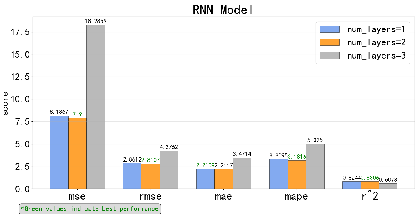
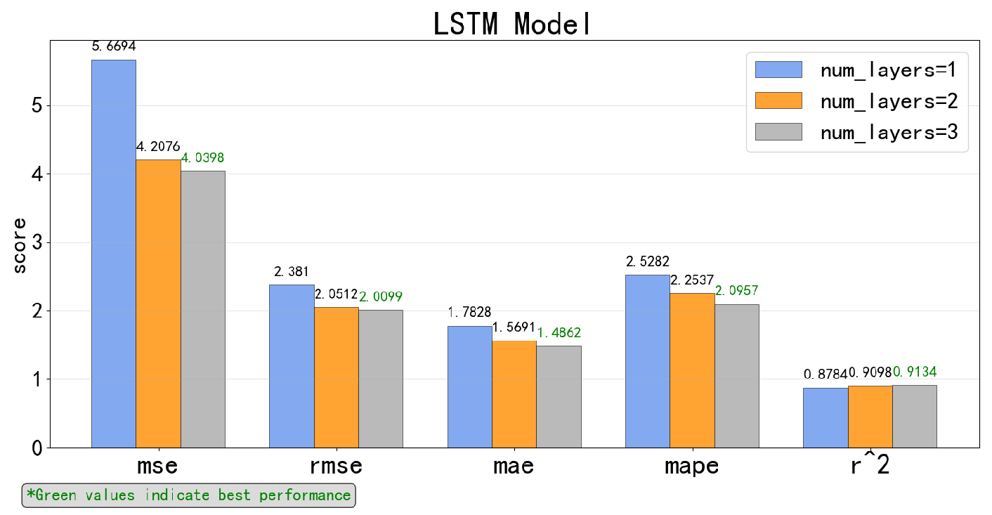
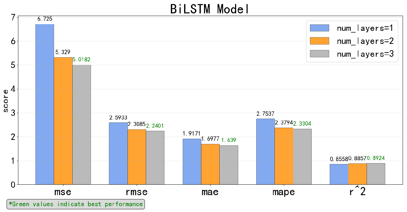
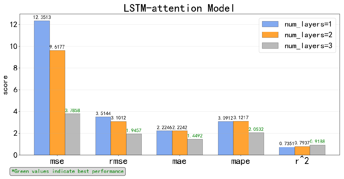
In this section, we report the respective results under different settings for each time-series deep learning model, which are depicted in Figure 5, Figure 6, Figure 7, Figure 8, Figure 9, Figure 10, Figure 11, Figure 12 and Figure 13.
Firstly, we use the White Shark Optimization Algorithm (WSO) to perform the first step of parameter coarse optimization on the nine deep learning models. After obtaining the parameter combinations of all models, we manually adjust them. We float the given parameters left and right to obtain the final optimal model. At the same time, the number of hidden layers, as a common model parameter among the nine depth models, can only be manually tested for each layer due to its small range of values. The following images show the results obtained from the nine depth models with different hidden layers.
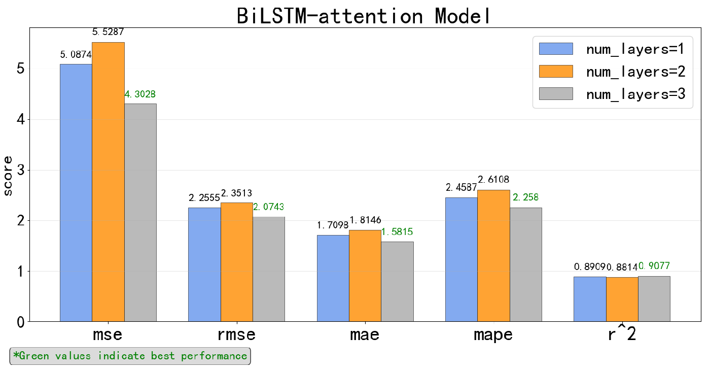
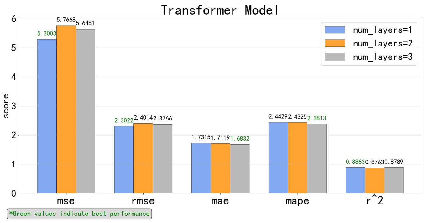
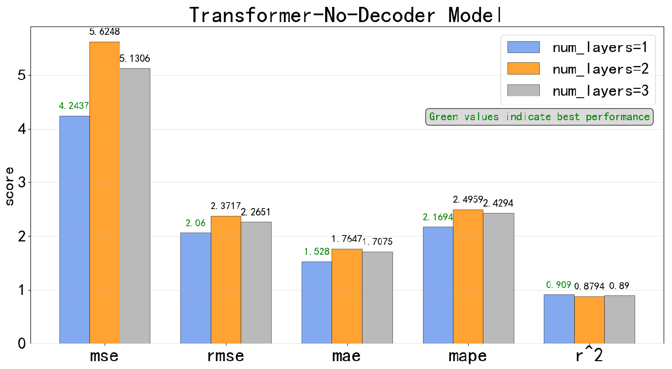
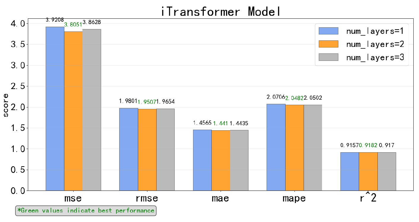
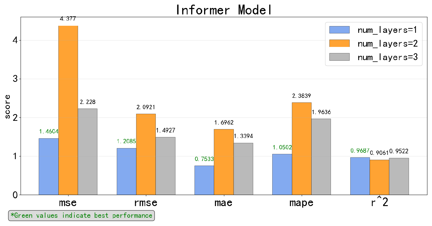
Figure 5 shows all the metrics mentioned above for the RNN-based SFC prediction model by adopting a different number of hidden layers. As we can see from the results, the MSE and R 2 score results show a similar ranking trend; i.e., if the result of a test option has a lower MSE compared to other option, then its R 2 score will be higher than that of the compared option. The best performance for RNN can be found when there are two hidden layers. Figure 6 shows the MSE and R 2 scores for the LSTM-based SFC prediction model by adopting a different number of hidden layers. The results of MSE and R 2 scores show a similar ranking trend, the same as the RNN’s results. The best performance for LSTM can be found when there are three hidden layers. Figure 7 shows the results for the BiLSTM-based model, whose MSE and R 2 score results also stay consistent. The best performance for BiLSTM occurs when the number of hidden layers is three. Figure 8 shows the results for the LSTM–attention-based model. The best performance for LSTM–attention can be found when there are three hidden layers. Then, Figure 9 shows that BiLSTM–attention and LSTM–attention have similar results. Figure 10 shows the results for the original Transformer-based model, whose MSE and R 2 score results also stay consistent. The best performance for the original Transformer is achieved when the number of hidden layers is three. Figure 11 shows the results for the Transformer-No-Decoder model, whose MSE and R 2 score results also stay consistent. The Transformer-NoDecoder provides the best prediction performance when the number of hidden layers is one. Figure 12 shows similar results for the iTransformer model, and its best setting is two hidden layers. Figure 13 shows the results for the Informer model, whose MSE and R 2 score results also stay consistent. The Informer predicted SFC most accurately with one hidden layer.
Summarizing this part of the experiment, we can find that the best parameters obtained by most time-series deep learning models with similar structures are also similar, which might indicate the similarity among the nearest ship energy efficiency data.

5.2.2. Comparison of Different Algorithms for SFC Prediction

The comparison results of using different prediction algorithms for the mixed model are shown in Figure 14. As we can see from it, the two result lines of MSE and R 2 scores demonstrate an opposite state, which indicates the same trend in the performance of different algorithms, as lower MSE and higher R 2 scores refer to better performance. Among the RNN-based models, LSTM–attention achieved the best performance in SFC prediction, with 3.79 and 0.919 for MSE and R 2 scores, respectively. The inferior performance of BiLSTM compared to LSTM indicates that the fuel consumption data of ships is not impacted by future information on current fuel consumption. Therefore, LSTM, which only considers historical data, performs better. However, BiLSTM still outperforms RNN, which also indicates that relatively complex dependencies exist in the energy efficiency data. Among them, the MSE obtained by the worst-performing RNN is also much lower than that of XGBoost, which indicates the temporal dependence of energy efficiency data recording and the importance of sequence. As can be seen from the chart, LSTM–attention has a slight edge over LSTM, which indicates that the attention mechanism helps optimize the results obtained by LSTM. However, the performance of Transformer and Transformer–No–Decoder did not surpass that of LSTM. There are already related studies questioning the effectiveness of Transformer in the time-series prediction field [61]. The reason behind this may be that Transformer-based models introduce time correlation through position encoding, which is significantly weaker in time-series modeling capability compared to other models. Then, the iTransformer, which is more suitable for time-series prediction, indeed meets expectations. Its performance is better than that of the LSTM–attention model, and it also proves that in the task of predicting ship fuel consumption, it is more crucial to deeply explore the intrinsic correlations between multivariate features than simply optimizing sequence modeling in the time dimension. The Informer model is a relatively new one and has achieved good results in multi-step prediction in the energy field. In this experiment, Informer was also the best-performing model, with 1.46 and 0.969 for MSE and R 2 scores. Compared with Transformer, Informer proposes PorbSpare self-attention, reducing the computational complexity to handle longer time series. It explicitly models using the distillation mechanism to capture multi-scale dependencies; a generative decoder is proposed to obtain the output of long sequences to avoid the continuous accumulation of errors. In summary, Informer is the most suitable algorithm for the time-series prediction module in the hybrid model proposed for TL in this study.

5.2.3. Visualization of the SFC Prediction Result for Different Models

In order to compare the algorithms more deeply and figure out the specific prediction result, we visualize parts of the prediction values in this section for all algorithms. We have selected 50 consecutive predicted values, and in order to represent them more clearly, we only choose the top 5 models in terms of predicted performance: LSTM, LSTM–attention, Transformer–No–Decoder, iTransformer, and Informer. They are shown in Figure 15. From the overall trend, the Informer model’s prediction curve has the highest degree of fit with the true value, almost achieving synchronous fluctuations, indicating excellent prediction accuracy and timeliness. In contrast, although the prediction curves of other models can capture the general trend of the true values, there is a significant lag phenomenon, with peaks and valleys always appearing several time steps later than the true values. In addition to the Informer model, we can see that the predicted values of the LSTM–attention mixed model are closer to the true values. Although the overall curve fluctuation of LSTM is closer to the real curve, there is a certain gap between the basic and real values. The accuracy of its results cannot be compared to Informer and LSTM–attention. It is sufficient to prove that the attention mechanism can optimize LSTM models. Therefore, the Informer model performs the best in predicting ship fuel consumption, as it can most effectively capture long-term dependencies in time series, avoiding the prediction lag problem that other models may encounter, thus achieving the closest prediction results to reality.

6. Conclusions and Future Work

Our research still has certain limitations. We only used a limited dataset, and future research can expand the experimental scope to include various types of ships, design prediction frameworks and models, and enhance the generalization ability of prediction models. And the data accuracy is insufficient. If the data accuracy can reach one line per second, the model accuracy will also increase. At the same time, there are high requirements for the dataset, which requires the ship to navigate the entire journey without any abnormal interruption of data. However, in reality, ship navigation data is bound to be filled with noise, which imposes a significant burden on data cleaning.
In this paper, we firstly analyzed the SFC prediction task from the perspective of the characteristics of ship energy efficiency data and then explored three groups of time-series models, RNN-based (RNN, LSTM, and BiLSTM), attention-based (Transformer, Transformer–No–Decoder, iTransformer, and Informer), and RNN–attention mixed (LSTM–attention and BiLSTM–attention), totaling nine models to predict SFCs. We proposed for the first time the application of Transformer- and Informer-related models to the prediction of ship fuel consumption, and we evaluated their performance experimentally by first searching for the proper settings for each algorithm and then comparing their MSE and R 2 scores. We also implemented an SFC prediction model based on XGBoost and compared its performance with all time-series models. The results showed that Informer outperforms other models for our ship energy efficiency data. Attention-based models are clearly of significant help for SFC prediction, and they also perform differently in LSTM, Transformer, and Informer. Among them, iTransformer proposed reversing the data dimension, which indeed improved the performance of the Transformer model, but still did not surpass Informer. In future work, we will explore whether the process of reversing data dimensions can be combined with Informer to further enhance the prediction results of SFC.
Our research demonstrates the superiority of the Informer model in predicting ship fuel consumption. Its practical value lies in its ability to provide accurate multi-step fuel consumption prediction for maritime departments, which directly translates into significant operational benefits: by optimizing speed and route selection, fuel consumption and corresponding carbon emissions can be reduced by 3–5%; based on prediction bias, early detection of ship hull fouling or equipment abnormalities can be achieved, enabling preventive maintenance; and data-driven decision support for fuel procurement, voyage cost accounting, and carbon emission compliance can be simultaneously provided, comprehensively enhancing the economic and environmental efficiency of ship operations.

Author Contributions

X.C.: writing—original draft, writing—review and editing, methodology, conceptualization, and investigation. X.L.: writing—original draft, methodology, software, and investigation. Y.L.: methodology and investigation. X.Z.: funding acquisition, supervision, and data curation. All authors have read and agreed to the published version of the manuscript.

Funding

This work was supported by the Science & Technology Commission of Shanghai Municipality and Shanghai Engineering Research Center of Ship Intelligent Maintenance and Energy Efficiency under Grant 20DZ2252300.

Data Availability Statement

The data presented in this study are not publicly available due to privacy and confidentiality restrictions.

Conflicts of Interest

The authors declare no conflicts of interest.

References

  1. Agand, P.; Kennedy, A.; Harris, T.; Bae, C.; Chen, M.; Park, E.J. Fuel consumption prediction for a passenger ferry using machine learning and in-service data: A comparative study. Ocean. Eng. 2023, 284, 115271. [Google Scholar] [CrossRef]
  2. Eide, M.S.; Longva, T.; Hoffmann, P.; Endresen, Ø.; Dalsøren, S.B. Future cost scenarios for reduction of ship CO2 emissions. Marit. Policy Manag. 2011, 38, 11–37. [Google Scholar] [CrossRef]
  3. Zeng, X.; Chen, M. A novel big data collection system for ship energy efficiency monitoring and analysis based on BeiDou system. J. Adv. Transp. 2021, 2021, 9914720. [Google Scholar] [CrossRef]
  4. IMO. IMO Regulations to Introduce Carbon Intensity Measures Enter into Force on 1 November 2022; Manifold Times: Singapore, 2022. [Google Scholar]
  5. Zeng, X.; Chen, M.; Li, H.; Wu, X. A data-driven intelligent energy efficiency management system for ships. IEEE Intell. Transp. Syst. Mag. 2022, 15, 270–284. [Google Scholar] [CrossRef]
  6. Mou, X.; Yuan, Y.; Yan, X.; Zhao, G. A Prediction Model of Fuel Consumption for Inland River Ships Based on Random Forest Regression. J. Transp. Inf. Saf. 2017, 35, 100–105. [Google Scholar]
  7. Hu, Z.; Zhou, T.; Osman, M.T.; Li, X.; Jin, Y.; Zhen, R. A novel hybrid fuel consumption prediction model for ocean-going container ships based on sensor data. J. Mar. Sci. Eng. 2021, 9, 449. [Google Scholar] [CrossRef]
  8. Yan, R.; Wang, S.; Du, Y. Development of a two-stage ship fuel consumption prediction and reduction model for a dry bulk ship. Transp. Res. Part Logist. Transp. Rev. 2020, 138, 101930. [Google Scholar] [CrossRef]
  9. Gkerekos, C.; Lazakis, I.; Theotokatos, G. Machine learning models for predicting ship main engine Fuel Oil Consumption: A comparative study. Ocean. Eng. 2019, 188, 106282. [Google Scholar] [CrossRef]
  10. Chen, Z.S.; Lam, J.S.L.; Xiao, Z. Prediction of harbour vessel fuel consumption based on machine learning approach. Ocean. Eng. 2023, 278, 114483. [Google Scholar] [CrossRef]
  11. Coraddu, A.; Oneto, L.; Baldi, F.; Anguita, D. Vessels fuel consumption forecast and trim optimisation: A data analytics perspective. Ocean. Eng. 2017, 130, 351–370. [Google Scholar] [CrossRef]
  12. Xie, X.; Sun, B.; Li, X.; Olsson, T.; Maleki, N.; Ahlgren, F. Fuel consumption prediction models based on machine learning and mathematical methods. J. Mar. Sci. Eng. 2023, 11, 738. [Google Scholar] [CrossRef]
  13. Bialystocki, N.; Konovessis, D. On the estimation of ship’s fuel consumption and speed curve: A statistical approach. J. Ocean. Eng. Sci. 2016, 1, 157–166. [Google Scholar] [CrossRef]
  14. Uyanık, T.; Karatuğ, Ç.; Arslanoğlu, Y. Machine learning approach to ship fuel consumption: A case of container vessel. Transp. Res. Part Transp. Environ. 2020, 84, 102389. [Google Scholar] [CrossRef]
  15. Soner, O.; Akyuz, E.; Celik, M. Statistical modelling of ship operational performance monitoring problem. J. Mar. Sci. Technol. 2019, 24, 543–552. [Google Scholar] [CrossRef]
  16. Soner, O.; Akyuz, E.; Celik, M. Use of tree based methods in ship performance monitoring under operating conditions. Ocean. Eng. 2018, 166, 302–310. [Google Scholar] [CrossRef]
  17. Tran, T.A. Comparative analysis on the fuel consumption prediction model for bulk carriers from ship launching to current states based on sea trial data and machine learning techniquec. J. Ocean. Eng. Sci. 2021, 6, 317–339. [Google Scholar] [CrossRef]
  18. Kim, Y.R.; Jung, M.; Park, J.B. Development of a fuel consumption prediction model based on machine learning using ship in-service data. J. Mar. Sci. Eng. 2021, 9, 137. [Google Scholar] [CrossRef]
  19. Zhou, T.; Hu, Q.; Hu, Z.; Zhen, R. An adaptive hyper parameter tuning model for ship fuel consumption prediction under complex maritime environments. J. Ocean. Eng. Sci. 2022, 7, 255–263. [Google Scholar] [CrossRef]
  20. Karagiannidis, P.; Themelis, N. Data-driven modelling of ship propulsion and the effect of data pre-processing on the prediction of ship fuel consumption and speed loss. Ocean. Eng. 2021, 222, 108616. [Google Scholar] [CrossRef]
  21. Jeon, M.; Noh, Y.; Shin, Y.; Lim, O.K.; Lee, I.; Cho, D. Prediction of ship fuel consumption by using an artificial neural network. J. Mech. Sci. Technol. 2018, 32, 5785–5796. [Google Scholar] [CrossRef]
  22. Bui-Duy, L.; Vu-Thi-Minh, N. Utilization of a deep learning-based fuel consumption model in choosing a liner shipping route for container ships in Asia. Asian J. Shipp. Logist. 2021, 37, 1–11. [Google Scholar] [CrossRef]
  23. Karatuğ, Ç.; Tadros, M.; Ventura, M.; Soares, C.G. Strategy for ship energy efficiency based on optimization model and data-driven approach. Ocean. Eng. 2023, 279, 114397. [Google Scholar] [CrossRef]
  24. Zhu, Y.; Zuo, Y.; Li, T. Predicting ship fuel consumption based on lstm neural network. In Proceedings of the 2020 7th International Conference on Information, Cybernetics, and Computational Social Systems (ICCSS), Guangzhou, China, 13–15 November 2020; IEEE: Piscataway, NJ, USA, 2020; pp. 310–313. [Google Scholar]
  25. Panapakidis, I.; Sourtzi, V.M.; Dagoumas, A. Forecasting the fuel consumption of passenger ships with a combination of shallow and deep learning. Electronics 2020, 9, 776. [Google Scholar] [CrossRef]
  26. Yuan, Z.; Liu, J.; Zhang, Q.; Liu, Y.; Yuan, Y.; Li, Z. Prediction and optimisation of fuel consumption for inland ships considering real-time status and environmental factors. Ocean. Eng. 2021, 221, 108530. [Google Scholar] [CrossRef]
  27. Chen, Y.; Sun, B.; Xie, X.; Li, X.; Li, Y.; Zhao, Y. Short-term forecasting for ship fuel consumption based on deep learning. Ocean. Eng. 2024, 301, 117398. [Google Scholar] [CrossRef]
  28. Zhang, M.; Tsoulakos, N.; Kujala, P.; Hirdaris, S. A deep learning method for the prediction of ship fuel consumption in real operational conditions. Eng. Appl. Artif. Intell. 2024, 130, 107425. [Google Scholar] [CrossRef]
  29. Lim, B.; Zohren, S. Time-series forecasting with deep learning: A survey. Philos. Trans. R. Soc. 2021, 379, 20200209. [Google Scholar] [CrossRef] [PubMed]
  30. Wen, Q.; Zhou, T.; Zhang, C.; Chen, W.; Ma, Z.; Yan, J.; Sun, L. Transformers in time series: A survey. arXiv 2022, arXiv:2202.07125. [Google Scholar]
  31. Scikit Learn. Metrics and Scoring: Quantifying the Quality of Predictions. 2023. Available online: https://scikit-learn.org/stable/modules/model_evaluation.html (accessed on 28 October 2025).
  32. Chai, T.; Draxler, R.R. Root mean square error (RMSE) or mean absolute error (MAE)?—Arguments against avoiding RMSE in the literature. Geosci. Model Dev. 2014, 7, 1247–1250. [Google Scholar] [CrossRef]
  33. Lewinson, E. A Comprehensive Overview of Regression Evaluation Metrics. 2023. Available online: https://developer.nvidia.com/blog/a-comprehensive-overview-of-regression-evaluation-metrics/ (accessed on 28 October 2025).
  34. Fan, A.; Yang, J.; Yang, L.; Wu, D.; Vladimir, N. A review of ship fuel consumption models. Ocean. Eng. 2022, 264, 112405. [Google Scholar] [CrossRef]
  35. Wang, S.; Meng, Q. Sailing speed optimization for container ships in a liner shipping network. Transp. Res. Part Logist. Transp. Rev. 2012, 48, 701–714. [Google Scholar] [CrossRef]
  36. Wei, N.; Yin, L.; Li, C.; Li, C.; Chan, C.; Zeng, F. Forecasting the daily natural gas consumption with an accurate white-box model. Energy 2021, 232, 121036. [Google Scholar] [CrossRef]
  37. Baldi, F. Modelling, Analysis and Optimisation of Ship Energy Systems; Chalmers University of Technology Gothenburg: Göteborg, Sweden, 2016. [Google Scholar]
  38. Kim, Y.; Emery, S.L.; Vera, L.; David, B.; Huang, J. At the speed of Juul: Measuring the Twitter conversation related to ENDS and Juul across space and time (2017–2018). Tob. Control 2021, 30, 137–146. [Google Scholar] [CrossRef]
  39. Yan, R.; Wang, S.; Psaraftis, H.N. Data analytics for fuel consumption management in maritime transportation: Status and perspectives. Transp. Res. Part Logist. Transp. Rev. 2021, 155, 102489. [Google Scholar] [CrossRef]
  40. Aldous, L.G. Ship Operational Efficiency: Performance Models and Uncertainty Analysis. Ph.D. Thesis, UCL (University College London), London, UK, 2016. [Google Scholar]
  41. Weiqiang, Y.; Honggui, L. Application of grey theory to the prediction of diesel consumption of diesel generator set. In Proceedings of the 2013 IEEE International Conference on Grey systems and Intelligent Services (GSIS), Macao, China, 15–17 November 2013; IEEE: Piscataway, NJ, USA, 2013; pp. 151–153. [Google Scholar]
  42. Sagi, O.; Rokach, L. Ensemble learning: A survey. Wiley Interdiscip. Rev. Data Min. Knowl. Discov. 2018, 8, e1249. [Google Scholar] [CrossRef]
  43. Freund, Y.; Schapire, R.E. Experiments with a new boosting algorithm. In Proceedings of the Thirteenth International Conference (ICML’96), Bari, Italy, 3–6 July 1996; Volume 96, pp. 148–156. [Google Scholar]
  44. Han, P.; Ellefsen, A.L.; Li, G.; Æsøy, V.; Zhang, H. Fault Prognostics Using LSTM Networks: Application to Marine Diesel Engine. IEEE Sens. J. 2021, 21, 25986–25994. [Google Scholar] [CrossRef]
  45. Liu, Y.; Gan, H.; Cong, Y.; Hu, G. Research on fault prediction of marine diesel engine based on attention-LSTM. Proc. Inst. Mech. Eng. Part J. Eng. Marit. Environ. 2023, 237, 508–519. [Google Scholar] [CrossRef]
  46. Park, H.J.; Lee, M.S.; Park, D.I.; Han, S.W. Time-Aware and Feature Similarity Self-Attention in Vessel Fuel Consumption Prediction. Appl. Sci. 2021, 11, 11514. [Google Scholar] [CrossRef]
  47. Li, J.; Cheng, K.; Wang, S.; Morstatter, F.; Trevino, R.P.; Tang, J.; Liu, H. Feature selection: A data perspective. Acm Comput. Surv. (CSUR) 2017, 50, 1–45. [Google Scholar] [CrossRef]
  48. Du, Y.; Meng, Q.; Wang, S.; Kuang, H. Two-phase optimal solutions for ship speed and trim optimization over a voyage using voyage report data. Transp. Res. Part Methodol. 2019, 122, 88–114. [Google Scholar] [CrossRef]
  49. Yu, Y.; Si, X.; Hu, C.; Zhang, J. A review of recurrent neural networks: LSTM cells and network architectures. Neural Comput. 2019, 31, 1235–1270. [Google Scholar] [CrossRef]
  50. Sherstinsky, A. Fundamentals of recurrent neural network (RNN) and long short-term memory (LSTM) network. Phys. D Nonlinear Phenom. 2020, 404, 132306. [Google Scholar] [CrossRef]
  51. Graves, A.; Schmidhuber, J. Framewise phoneme classification with bidirectional LSTM and other neural network architectures. Neural Netw. 2005, 18, 602–610. [Google Scholar] [CrossRef]
  52. Huang, Z.; Xu, W.; Yu, K. Bidirectional LSTM-CRF models for sequence tagging. arXiv 2015, arXiv:1508.01991. [Google Scholar] [CrossRef]
  53. Vaswani, A.; Shazeer, N.; Parmar, N.; Uszkoreit, J.; Jones, L.; Gomez, A.N.; Kaiser, L.; Polosukhin, I. Attention is all you need. In Proceedings of the 31st International Conference on Neural Information Processing Systems, Long Beach, CA, USA, 4–9 December 2017; Curran Associates Inc.: Red Hook, NY, USA, 2017. NIPS’17. pp. 6000–6010. [Google Scholar]
  54. Li, Z.; Rao, Z.; Pan, L.; Xu, Z. Mts-mixers: Multivariate time series forecasting via factorized temporal and channel mixing. arXiv 2023, arXiv:2302.04501. [Google Scholar] [CrossRef]
  55. Lin, S.; Lin, W.; Wu, W.; Wang, S.; Wang, Y. Petformer: Long-term time series forecasting via placeholder-enhanced transformer. IEEE Trans. Emerg. Top. Comput. Intell. 2024, 9, 1189–1201. [Google Scholar] [CrossRef]
  56. Liu, Y.; Hu, T.; Zhang, H.; Wu, H.; Wang, S.; Ma, L.; Long, M. iTransformer: Inverted Transformers Are Effective for Time Series Forecasting. arXiv 2023, arXiv:2310.06625. [Google Scholar]
  57. Gong, M.; Zhao, Y.; Sun, J.; Han, C.; Sun, G.; Yan, B. Load forecasting of district heating system based on Informer. Energy 2022, 253, 124179. [Google Scholar] [CrossRef]
  58. Zhu, Q.; Han, J.; Chai, K.; Zhao, C. Time series analysis based on informer algorithms: A survey. Symmetry 2023, 15, 951. [Google Scholar] [CrossRef]
  59. Yang, Z.; Liu, L.; Li, N.; Tian, J. Time series forecasting of motor bearing vibration based on informer. Sensors 2022, 22, 5858. [Google Scholar] [CrossRef] [PubMed]
  60. Zhou, H.; Zhang, S.; Peng, J.; Zhang, S.; Li, J.; Xiong, H.; Zhang, W. Informer: Beyond efficient transformer for long sequence time-series forecasting. In Proceedings of the AAAI Conference on Artificial Intelligence, Virtual Event, 19–21 May 2021; Volume 35, pp. 11106–11115. [Google Scholar]
  61. Zeng, A.; Chen, M.; Zhang, L.; Xu, Q. Are transformers effective for time series forecasting? In Proceedings of the AAAI Conference on Artificial Intelligence, Washington, DC, USA, 7–14 February 2023; Volume 37, pp. 11121–11128. [Google Scholar]
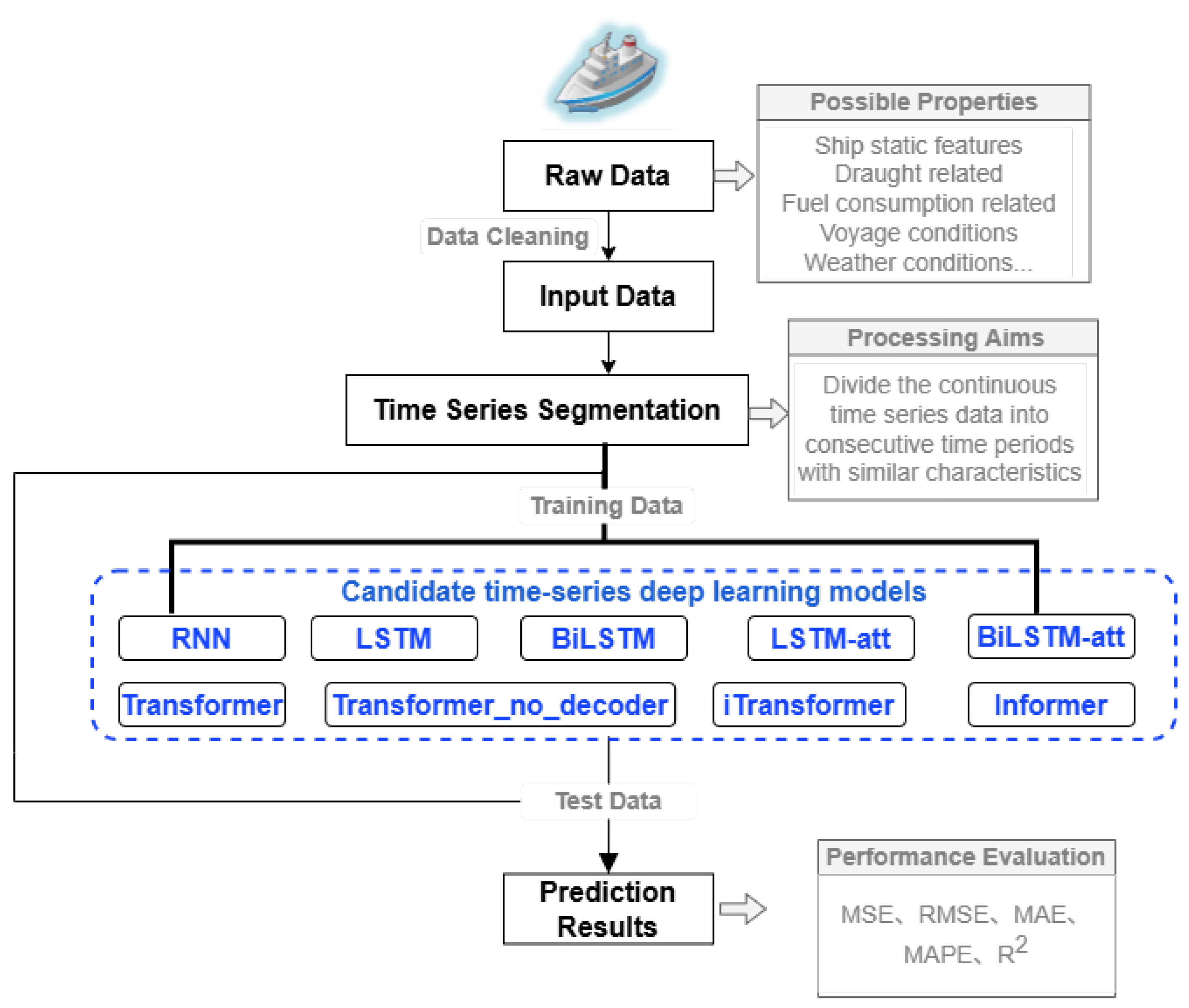
Figure 1. The overall process using nine possible time-series deep learning models for SFC prediction.
Jmse 13 02102 g001
Figure 2. RNN-based model structure comparisons [49,50,51,52].
Jmse 13 02102 g002
Figure 4. The combination of BiLSTM and attention [28].
Jmse 13 02102 g004
Figure 5. RNN-based models.
Jmse 13 02102 g005
Figure 6. LSTM-based models.
Jmse 13 02102 g006
Figure 7. BiLSTM-based models.
Jmse 13 02102 g007
Figure 8. LSTM–attention-based models.
Jmse 13 02102 g008
Figure 9. BiLSTM–attention-based models.
Jmse 13 02102 g009
Figure 10. Transformer-based models.
Jmse 13 02102 g010
Figure 11. Transformer–No–Decoder models.
Jmse 13 02102 g011
Figure 12. Transformer-based models.
Jmse 13 02102 g012
Figure 13. Informer-based models.
Jmse 13 02102 g013
Figure 14. MSE and R 2 score comparison of different algorithms.
Jmse 13 02102 g014
Figure 15. Visualization of SFC prediction values of different models.
Jmse 13 02102 g015
Table 1. Calculated features based on raw features.
NameUnitCalculation Equation
F C m e kg/km C o n s u m p t i o n i n p u t C o n s u m p t i o n o u t p u t S h i p S p d T o W a t e r
ShipSlip% ( 1 S h i p S p d T o W a t e r 60 M E R p m p i t c h   * ) 100
ShipTrimm S h i p D r a u g h t A s t e r n S h i p D r a u g h t B o w
ShipHeelm S h i p D r a u g h t M i d L f t S h i p D r a u g h t M i d R g t
* pitch: propeller pitch.
Disclaimer/Publisher’s Note: The statements, opinions and data contained in all publications are solely those of the individual author(s) and contributor(s) and not of MDPI and/or the editor(s). MDPI and/or the editor(s) disclaim responsibility for any injury to people or property resulting from any ideas, methods, instructions or products referred to in the content.