Physics-Informed Dynamics Modeling: Accurate Long-Term Prediction of Underwater Vehicles with Hamiltonian Neural ODEs

Abstract

Accurately predicting the long-term behavior of complex dynamical systems is a central challenge for safety-critical applications like autonomous navigation. Mechanistic models are often brittle, relying on difficult-to-measure parameters, while standard deep learning models are black boxes that fail to generalize, producing physically inconsistent predictions. Here, we introduce a physics-informed framework that learns the continuous-time dynamics of an Autonomous Underwater Vehicle (AUV) by discovering its underlying energy landscape. We embed the structure of Port-Hamiltonian mechanics into a neural ordinary differential equation (NODE) architecture, learning not to imitate trajectories but rather to identify the system’s Hamiltonian and its constituent physical matrices from observational data. Geometric consistency is enforced by representing rotational dynamics on the SE(3) manifold, preventing numerical error accumulation. Experimental validation reveals a stark performance divide. While a state-of-the-art black-box model matches our accuracy in simple, interpolative maneuvers, its predictions fail catastrophically under complex controls. Quantitatively, our physics-informed model maintained a mean 10 s position error of a mere 3.3 cm, whereas the black-box model’s error diverged to 5.4 m—an over 160-fold performance gap. This work establishes that the key to robust, generalizable models lies not in bigger data or deeper networks but in the principled integration of physical laws, providing a clear path to overcoming the brittleness of black-box models in critical engineering simulations.

1. Introduction

Autonomous Underwater Vehicles (AUVs) are unmanned ocean observation platforms with intelligence. They are known for their compact size, high maneuverability, and ability to operate in deep-sea environments. AUVs incorporate various sensors enabling them to carry out thorough surveys and research in underwater environments, which allows them to undertake submersible exploration without temporal and spatial constraints.

In marine science, AUVs collect oceanic environmental data, survey seafloor geology and topography, and prospect for resources like oil. In marine engineering, AUVs evaluate dam structures, help maintain underwater foundations, aid divers with their tasks, and perform underwater target observation, search, and rescue missions. In military applications, AUVs detect targets, collect intelligence, perform surveillance and reconnaissance, and engage in anti-submarine warfare and related activities.

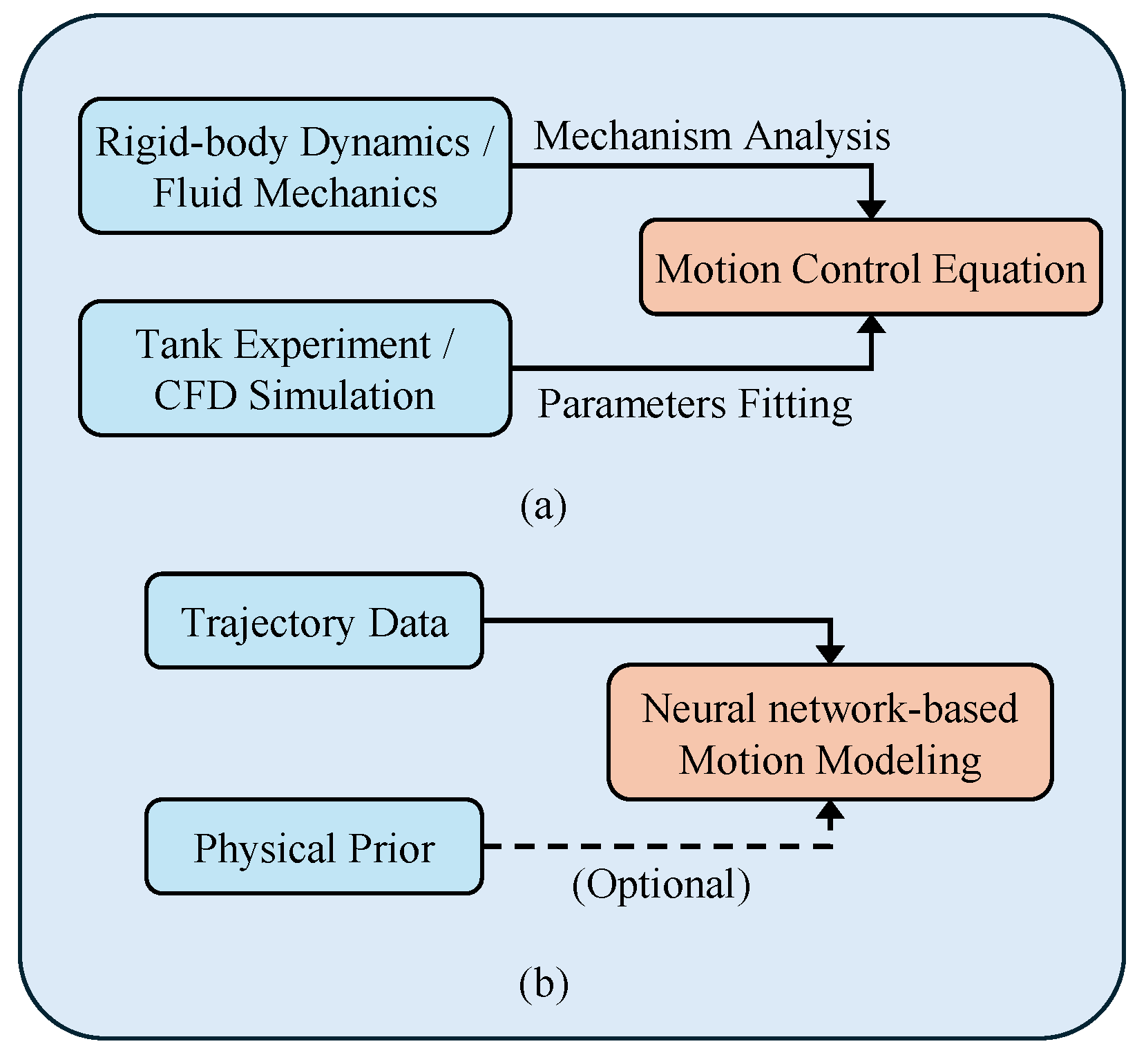
Differential equations are typically used to describe the motion model of an underwater vehicle. For a particular type of underwater vehicle, Figure 1 illustrates how certain parameters in the motion equations, like the inertial matrix and the Coriolis–centripetal moment matrix, among others, can be accurately obtained through experimental measurements or theoretical calculations once the interior structure and exterior design are established. Nevertheless, another set of parameters, such as hydrodynamic damping coefficients, require acquisition through computational fluid dynamics (CFD) simulations or water tank experiments, despite the fact that the resulting values frequently display a certain degree of discrepancy from the actual ones [1].

Considerable research has focused on overcoming the challenge of estimating inaccurate hydrodynamic parameters. System identification methods have emerged as a common pathway for obtaining high-precision hydrodynamic parameters among various approaches. This method enables a cost-effective online or offline identification of parameters. To identify and optimize parameters, the fundamental approach involves designing parameter identification experiments and subsequently utilizing techniques such as the least squares method [2], Kalman filtering [3], Gaussian processes [4], or neural networks [5].

System identification can attain the desired accuracy by minimizing the discrepancy between theoretical models and actual data [6]. Nevertheless, these methods have some limitations. Firstly, the accuracy of system identification methods depends on the quality of the theoretical model used. In situations where the model is faulty, accurate motion models can still be hard to achieve, even if the identification method shows high precision. Secondly, to completely excite the dynamic characteristics of underwater vehicles, tailored parameter identification experiments must be designed. This leads to a considerable need for high-quality trajectory data. Lastly, when multiple parameters need identification, it may cause challenges for algorithm convergence. It becomes necessary to decouple the motion of the underwater vehicle followed by identifying hydrodynamic parameters in separate channels. Nevertheless, this method may result in inaccuracies when estimating strongly coupled parameters.

Moreover, the theoretical model may lack accuracy inherently because of the absence of a universally accepted method for modeling hydrodynamic damping terms. Numerous methods have been summarized in reference [7] with varying assumptions made regarding the vehicle and fluid characteristics. The generated models differ in their applicability and computational complexity across various scenarios. Furthermore, certain factors within the vehicle dynamics model, including manufacturing errors, assembly discrepancies, external disturbances, and changes in physical characteristics over time, present challenges for explicit modeling. Therefore, predicting the motion behavior of underwater vehicles through differential equations to obtain long-term accurate explanations is exceedingly difficult. Establishing a motion model through experiments, even with a lot of effort, is only applicable to a specific type of vehicle and is difficult to generalize to other vehicles.

Recently, deep learning technology has seen rapid development and has been extensively applied in various fields, including visual recognition [8], natural language understanding [9], robot manipulation, and control [10]. Deep learning has demonstrated much better performance than traditional methods. Deep neural networks are theoretically capable of fitting any nonlinear function, as they serve as universal function approximators. Deep neural networks can automatically extract latent features from large amounts of data, which is supported by carefully designed network architectures and advanced training strategies.

Modeling underwater vehicle dynamics through theoretical analysis presents challenges due to the inherent incompleteness of theoretical models and difficulties associated with obtaining certain parameters accurately. In contrast, deep learning methods can effectively utilize the impressive fitting capacity of neural networks. These methods learn the dynamics of underwater vehicles directly from their trajectory data, surpassing the mere task of fitting parameters within theoretical models.

It is important to note that deep neural networks are black-box models and lack interpretability in their operational mechanisms. Although deep neural networks usually have high model capacity to fit training data well, they may not capture the true underlying patterns in some cases. Instead, they may identify specific local optimal solutions. When confronted with scenarios outside the training data, such models can exhibit significant performance degradation, which is commonly referred to as over-fitting.

To enhance the generalization ability of deep neural networks in unfamiliar contexts and to guide their learning of appropriate data patterns, it is necessary to incorporate task-relevant prior information, i.e., biases, into the learning process. The embedding of bias information into neural networks can be categorized into the following three approaches: a. Input bias: During the data pre-processing stage, domain knowledge can be used to normalize the data by bringing different scales of data to the same. If the data distribution is unfavorable, domain knowledge can be applied to adjust the data distribution, thus facilitating a more effective modeling of the target area [11]. b. Inductive bias: Designing specialized neural network architectures for specific tasks is one way to implicitly embed prior information into the learning process. For example, convolutional neural networks exploit the symmetry and distributed pattern representation present in natural images. By using network structures based on local connectivity and parameter sharing, they have revolutionized the field of computer vision [12,13,14,15]. c. Learning bias: Incorporating task-relevant prior information into the loss function as penalty terms is another strategy. This is similar to multi-task learning, where the learning algorithm not only adapts to the training data but also ensures that the network predictions satisfy certain constraints (e.g., conservation of quality and momentum, monotonicity, etc.). Typical methods include deep Galerkin methods [16] and physics-informed neural networks [17,18].

In addition, traditional neural network methods often deal only with discrete data, while the sampling intervals of actual motion data may be irregular. The challenge of recovering continuous dynamics of underwater vehicles from such observational data remains another critical issue. In this study, we establish the neural ordinary differential equation (neural ODE) [19] as a fundamental framework to modeling underwater vehicle dynamics. This framework combines ordinary differential equations with neural networks, starting only from the initial state of the system and using non-uniform observation data to model continuous dynamics. We then express the motion model of underwater vehicles in the form of Hamiltonian mechanics, using the Hamiltonian neural network (HNN) to model system conservation and dissipation quantities, respectively [20,21]. By using exponential mapping methods to handle rotational motion, we ensure that the resulting motion model satisfies the dynamic constraints of underwater vehicles. Finally, we compare the derived dynamic model to a fully data-driven modeling method. The experimental results show that our proposed modeling approach has significant advantages in terms of model robustness and long-term prediction accuracy.

The key contributions of this work are therefore threefold:

• We propose a novel physics-informed framework for AUV dynamics modeling that integrates a Port-Hamiltonian structure within a neural ordinary differential equation (NODE) to explicitly separate and learn energy-conserving and dissipative effects from data.
• We ensure geometric consistency and numerical stability for long-term prediction by representing the full 6-DOF rigid-body motion on the SE(3) manifold, which inherently respects the constraints of rotational dynamics and avoids singularities.
• We provide rigorous quantitative evidence demonstrating that our physics-informed approach overcomes the inherent brittleness of black-box models, maintaining high-fidelity predictions in complex, out-of-distribution scenarios where purely data-driven methods fail.

The paper is organized as follows. Section 2 provides some preliminaries of this work. Section 3 describes the proposed method for the dynamic modeling of underwater vehicles. Experimental results and the discussion are presented in Section 4. And the conclusion is given in Section 5.

2. Sequence Modeling Based on Neural Ordinary Differential Equations

2.1. Problem Statement

We can conceptualize the motion modeling of underwater vehicles as a time series prediction problem. Let us assume that at time t, the motion state of the underwater vehicle can be represented by a vector ${\mathit{x}}_t$ containing both position and velocity information. Therefore, within the time interval from $t=0$ to $t=T$, the changing motion states form a sequence $\mathit{X}=\left({\mathit{x}}_0,{\mathit{x}}_1,\dots ,{\mathit{x}}_T\right)$. For simplicity, we assume that the control inputs of the underwater vehicle remain constant during this period. As a result, the motion modeling problem for the underwater vehicle revolves around predicting a sequence of motion states $\mathit{Y}=\left({\mathit{x}}_{T+1},{\mathit{x}}_{T+2},\dots ,{\mathit{x}}_{T+N}\right)$ for a duration from time $T+1$ to $T+N$ based on the known sequence $\mathit{X}$.

In the context of deep learning, the time series prediction can be seen as a supervised learning problem, which allows us to express the above problem in a more general form. Given the sets $\mathcal{Y}:={\mathbb{R}}^{N\times L}$ and $\mathcal{X}:={\mathbb{R}}^{M\times L}$, sampled from an unknown distribution p, denoted as $\mathcal{D}\in \left(\mathcal{X}\times \mathcal{Y}\right)$, and a loss function $\mathcal{L}:=\mathcal{Y}\times \mathcal{Y}\to \mathbb{R}$, the goal is to find a function $\mathcal{F}:=\mathcal{X}\to \mathcal{Y}$ that minimizes the expected loss

$$min{\mathbb{E}}_{\left(\left(\mathit{x},\mathit{y}\right),{\mathit{y}}^{\prime }\right)\sim p}\left(\mathcal{L}\left({\mathit{y}}^{\prime },\mathcal{F}\left(\mathit{x},\mathit{y}\right)\right)\right),$$

(1)

where $\mathit{x}\in \mathcal{X}$ represents the known sequence, $\mathit{y},{\mathit{y}}^{\prime }\in \mathit{Y}$ are the predicted and target sequences, respectively, and the function $\mathcal{F}$ can be parameterized as a neural network that takes $\mathit{x}$ as input and produces $\mathit{y}$ as output. The goal is to minimize the expected loss given by the loss function $\mathcal{L}$, considering pairs of predicted and target sequences sampled from the distribution p.

Commonly used neural network architectures for time series modeling include recurrent neural networks (RNNs), long short-term memory networks (LSTMs), and the Transformer [22]. Among them, the Transformer has gained increasing attention due to its ability to capture long-term dependencies and interactions. Compared to RNNs and LSTMs, the Transformer can parallelize the processing of input sequences, providing computational advantages for large-scale data processing. Although these neural network models applied to sequence prediction may differ, they generally share similar architectural forms, as shown in Figure 2.

While these models have the advantages of simplicity and the ability to handle long-term or short-term dependencies, they are typically applied to uniformly sampled time series data. When applied to underwater vehicle motion modeling, it is often required that each state in the sequence has an equal time interval. Although the limitation of non-uniformly sampled data can be addressed by resampling or interpolation, these methods may compromise the original temporal information in the data. To avoid the loss of valuable information, another method is to include time stamps of the time series data as input to the neural network. However, compared to modeling methods based on differential equations, these methods still remain as discrete data modeling and may struggle to effectively model continuous dynamics.

2.2. Neural Ordinary Differential Equations

Neural ODE is a modeling method that combines ordinary differential equations with residual networks (ResNet) [8] to learn the dynamics of a system from data without having to explicitly define the differential equation. Unlike methods such as RNNs, neural ODEs require only the initial state of the system as input, eliminating the need for a sequence of data as input. This feature allows neural ODEs to naturally model time series data with non-uniform sampling and predict the dynamics of a system over continuous time.

As Figure 3 shows, the transformation of hidden states within a neural network can be expressed as

$$h\left(t+1\right)=f\left(h\left(t\right),\theta \left(t\right)\right),$$

(2)

where f represents a network layer, $h\left(t\right)$ and $\theta \left(t\right)$ denote the state output and weight matrix of layer t, and $h\left(t+1\right)$ represents the state output of layer $t+1$.

For residual networks, the expression is

$$h\left(t+1\right)=h\left(t\right)+f\left(h\left(t\right),\theta \left(t\right)\right),$$

(3)

where $h\left(t\right)$ can skip the network layer at $t+1$ and be added to the output.

To make the connection between the ODE and the residual network, consider a simple ordinary differential equation

$$y^{\prime }\left(t\right)=f\left(y,t\right).$$

(4)

Given an initial value $y\left(0\right)=y_0$ and a time step of 1, the iterative solution process can be expressed as

$$\begin{array}{cc}\hfill y\left(0\right)& =y_0\hfill \\ \hfill y\left(1\right)& =y\left(0\right)+y^{\prime }\left(0\right)\hfill \\ \hfill y\left(2\right)& =y\left(1\right)+y^{\prime }\left(1\right)\hfill \\ \hfill & ⋮\hfill \\ \hfill y\left(t\right)& =y\left(t-1\right)+y^{\prime }\left(t-1\right)\hfill \end{array}$$

(5)

This process is also known as Euler’s method for solving differential equations. If we consider the hidden layer index t in (4) as the time step t in (5), the forward propagation process of a ResNet has the same form as the iterative solution process of a differential equation.

However, there are two differences: (a) when solving an ODE, the time step can take any continuous value, while for ResNet, the time step is discrete, i.e., the number of network layers; (b) different residual blocks of ResNet have different f functions, while in an ODE, there is essentially a single f function defined by (5). Based on this, all residual blocks can be assigned the same parameters. In addition, since the time step is fixed, it can be chosen to be sufficiently small, allowing the network to become deep. As a result, a neural network based on an ODE with continuous depth can be formulated.

2.3. Hamiltonian Neural Networks

A neural ODE provides a general method for learning continuous-time dynamics from non-uniformly sampled data without imposing constraints on the underlying dynamical system. This provides versatility but also makes it difficult to accurately model specific physical processes. From a learning theory perspective, this is because a neural ODE has fewer inductive biases and lacks certain necessary assumptions about the target function to be learned.

Hamiltonian mechanics describes the evolution of the system state over time in phase space, where the system state is represented by generalized coordinates $\mathit{q}=\left(q_1,q_2,\dots ,q_n\right)\in {\mathbb{R}}^n$ and generalized moments $\mathit{p}=\left(p_1,p_2,\dots ,p_n\right)\in {\mathbb{R}}^n$. The Hamiltonian function $H:{\mathbb{R}}^{2n}\to \mathbb{R}$ maps the state of the system to a scalar representing the total energy of the system. In the context of classical mechanics, the Hamiltonian H represents the sum of the kinetic and potential energies of the system. The Hamiltonian function specifies a vector field in phase space that describes all possible dynamic behaviors of the system. Each state of the system corresponds to a unique trajectory in phase space.

The Hamiltonian function can be expressed as

$$H\left(\mathit{q},\mathit{p}\right)=T\left(\mathit{p}\right)+V\left(\mathit{q}\right),$$

(6)

where $T\left(\mathit{p}\right)$ is the kinetic energy and $V\left(\mathit{q}\right)$ is the potential energy. The evolution of the state of the system over time is described by the Hamiltonian equations

$${\displaystyle \frac{d\mathit{q}}{dt}}={\displaystyle \frac{\partial H}{\partial \mathit{p}}},{\displaystyle \frac{d\mathit{p}}{dt}}=-{\displaystyle \frac{\partial H}{\partial \mathit{q}}}.$$

(7)

The direction of the vector field defined by (7) is typically called the symplectic gradient of the Hamiltonian system.

It is easy to show that

$${\displaystyle \frac{dH}{dt}}={\displaystyle \frac{\partial H}{\partial \mathit{q}}}{\displaystyle \frac{d\mathit{q}}{dt}}+{\displaystyle \frac{\partial H}{\partial \mathit{p}}}{\displaystyle \frac{d\mathit{p}}{dt}}=0.$$

(8)

This implies that the total energy of the system is conserved when moving along the direction of the symplectic gradient [23].

In recent years, deep neural networks have been used to learn the Hamiltonian mechanics [24,25]. The Hamiltonian neural network is proposed to model the Hamiltonian function using deep neural networks and satisfy the dynamics of (7), ensuring that the system obeys the law of conservation of energy.

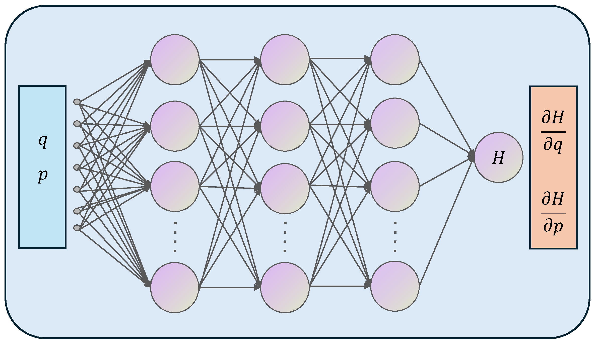
As Figure 4 shows, during forward computation, the HNN takes the generalized coordinates and momenta of the system as input and outputs the total energy of the system $H_{\theta }$, where $\theta$ represents the learnable network parameters. In the backpropagation process, the derivatives of the output with respect to the inputs are computed using automatic differentiation. The loss function of the HNN can be expressed as

$${\mathcal{L}}_{HNN}={∥{\displaystyle \frac{\partial H_{\theta }}{\partial \mathit{p}}}-{\displaystyle \frac{\partial \mathit{q}}{\partial t}}∥}_2+{∥{\displaystyle \frac{\partial H_{\theta }}{\partial \mathit{q}}}+{\displaystyle \frac{\partial \mathit{p}}{\partial t}}∥}_2.$$

(9)

Let

$${\mathit{S}}_H\left(\mathit{q},\mathit{p}\right)=\left({\displaystyle \frac{\partial H}{\partial \mathit{p}}},-{\displaystyle \frac{\partial H}{\partial \mathit{q}}}\right)$$

(10)

represent the dynamics of the system’s evolution over time. If the system state $\left({\mathit{q}}_0,{\mathit{p}}_0\right)$ at time $t_0$ is known, the neural ODE can be used to obtain the system state at time $t_1$,

$$\left({\mathit{q}}_1,{\mathit{p}}_1\right)=\left({\mathit{q}}_0,{\mathit{p}}_0\right)+{\int }_{t_0}^{t_1}{\mathit{S}}_H\left(\mathit{q},\mathit{p}\right)dt$$

(11)

Compared to the conventional neural ODE, the HNN offers faster training speeds, better generalization performance, and the ability to learn the dynamics of conservative systems more effectively.

3. Motion Modeling Based on Hamiltonian Neural Networks

3.1. Hamiltonian-Based Motion Equation

The kinematic model of an underwater vehicle can be expressed as

$$\dot{\mathit{\eta }}=\mathit{J}\left(\mathit{\eta }\right)\mathit{\nu },$$

(12)

where $\mathit{\eta }={({\mathit{p}}^n,\mathbf{\Theta })}^T={(x^n,y^n,z^n,\varphi ,\theta ,\psi )}^T$ represents the position and orientation vector in the Earth-fixed coordinate system {n}. Here, the Euler angles $\varphi ,\theta$, and $\psi$ correspond to the vehicle’s roll, pitch, and yaw, respectively. The vector $\mathit{\nu }={(\mathit{v},\mathit{\omega })}^T={(u,v,w,p,q,r)}^T$ represents the velocity vector in the body-fixed coordinate system {b}.

The coordinate transformation matrix $\mathit{J}\left(\mathit{\eta }\right)$ can be written as

$$\mathit{J}\left(\mathit{\eta }\right)=\left(\begin{array}{cc}{\mathit{J}}_1& {\mathbf{0}}_{3\times 3}\\ {\mathbf{0}}_{3\times 3}& {\mathit{J}}_2\end{array}\right),$$

(13)

where

$${\mathit{J}}_1=\left(\begin{array}{ccc}c\psi c\theta & -s\psi c\varphi +c\psi s\theta s\varphi & s\psi s\varphi +c\psi c\varphi s\theta \\ s\psi c\theta & c\psi c\varphi +s\varphi s\theta s\psi & -c\psi s\varphi +s\theta s\psi c\varphi \\ -s\theta & c\theta s\varphi & c\theta c\varphi \end{array}\right),$$

(14)

and

$${\mathit{J}}_2=\left(\begin{array}{ccc}1& s\varphi t\theta & c\varphi t\theta \\ 0& c\varphi & -s\varphi \\ 0& s\varphi /c\theta & c\varphi /c\theta \end{array}\right).$$

(15)

${\mathit{J}}_1$ denotes the rotation matrix, which can often be written as $\mathit{R}$, and $c(·)$, $s(·)$, and $t(·)$, respectively, denote $cos(·)$, $sin(·)$, and $tan(·)$.

The dynamic model of an underwater vehicle can be written as

$$\mathit{M}\dot{\mathit{\nu }}+\mathit{C}\left(\mathit{\nu }\right)\mathit{\nu }+\mathit{D}\left(\mathit{\nu }\right)\mathit{\nu }+\mathit{g}\left(\mathit{\eta }\right)=\mathit{\tau },$$

(16)

where $\mathit{M}={\mathit{M}}_{RB}+{\mathit{M}}_A$ represents the inertia matrix, ${\mathit{M}}_{RB}$ and ${\mathit{M}}_A$ denote the rigid body mass and hydrodynamic added mass, respectively. $\mathit{C}\left(\mathit{\nu }\right)={\mathit{C}}_{RB}\left(\mathit{\nu }\right)+{\mathit{C}}_A\left(\mathit{\nu }\right)$ defines the Coriolis and centripetal matrix. $\mathit{D}\left(\mathit{\nu }\right)$ is the hydrodynamic damping matrix. $\mathit{g}\left(\mathit{\eta }\right)$ represents the combined gravitational and buoyancy forces, while $\mathit{\tau }$ represents the control force vector.

In the case of small and low-speed underwater vehicles, several hydrodynamic effects can be considered negligible, leading to significant hydrodynamic model simplification [26,27,28]. According to [29], in an ideal fluid, ${\mathit{M}}_A$ can be expressed as a semi-positive definite matrix, and this characteristic holds true even in the case of real fluids. In the case of low-speed underwater vehicles, it is often possible to ignore the off-diagonal elements found in the ${\mathit{M}}_A$ matrix. The term ${\mathit{C}}_A\left(\mathit{\nu }\right)$ is always represented as an anti-symmetric matrix, where ${\mathit{C}}_A\left(\mathit{\nu }\right)=-{{\mathit{C}}_A\left(\mathit{\nu }\right)}^T$. The damping terms in high-speed underwater vehicles are highly nonlinear and coupled. Contributions from non-diagonal elements in the damping matrix are also typically negligible for low-speed vehicles.

Due to the influence of hydrodynamics and external control, the underwater vehicle is not a conservative system. Its motion can be described using the Port-Hamiltonian (PH) framework [30]. The PH equation can be written as

$$\left(\begin{array}{c}\dot{\mathit{q}}\\ \dot{\mathit{p}}\end{array}\right)=\left(\mathbf{J}\left(\mathit{q},\mathit{p}\right)-\mathbf{R}\left(\mathit{q},\mathit{p}\right)\right)\left(\begin{array}{c}{\displaystyle \frac{\partial H}{\partial \mathit{q}}}\\ {\displaystyle \frac{\partial H}{\partial \mathit{p}}}\end{array}\right)+\mathbf{G}\left(\mathit{q},\mathit{p}\right){\mathit{\tau }}_{ctrl},$$

(17)

where $\mathbf{J}\left(\mathit{q},\mathit{p}\right)$ is an anti-symmetric matrix describing the conservational aspects of the system. $\mathbf{R}\left(\mathit{q},\mathit{p}\right)$ is a positive definite matrix representing the dissipative effects. ${\mathit{\tau }}_{ctrl}$ is the control input, and $\mathbf{G}\left(\mathit{q},\mathit{p}\right){\mathit{\tau }}_{ctrl}$ describes external energy inputs. When there are no dissipative terms or external inputs, (17) can degenerate into the standard Hamiltonian equation.

The dynamic model of the underwater vehicle [31], the derivation of which is detailed in Appendix A, can be written as

$$\left(\begin{array}{c}\dot{\mathit{q}}\\ \dot{\mathit{p}}\end{array}\right)=\left(\left(\begin{array}{cc}0& \mathit{J}\\ -{\mathit{J}}^T& -\mathit{C}\end{array}\right)-\left(\begin{array}{cc}0& 0\\ 0& \mathit{D}\end{array}\right)\right)\left(\begin{array}{c}{\displaystyle \frac{\partial H}{\partial \mathit{q}}}\\ {\displaystyle \frac{\partial H}{\partial \mathit{p}}}\end{array}\right)+\left(\begin{array}{c}0\\ \mathit{I}\end{array}\right)\mathit{\tau },$$

(18)

where $\mathit{q}=\mathit{\eta }$, $\mathit{p}=\mathit{M}\mathit{\nu }$, and the Hamiltonian function can be expressed as

$$H={\displaystyle \frac{1}{2}}{\mathit{p}}^T{\mathit{M}}^{-1}\mathit{p}+V\left(\mathit{q}\right).$$

(19)

3.2. Representation of Rotational Motion

The orientation of underwater vehicles is typically represented by Euler angles. To unify the generalized coordinates in real space, the angle coordinates $\mathit{q}$ can be represented as a two-dimensional embedding $\left(cos\mathit{q},sin\mathit{q}\right)$ [23,32]. However, when dealing with the rotation of underwater vehicles, the exponential map provides a more effective solution. The exponential map is a method that maps angular velocity vectors to their corresponding rotation matrices and can be used to update the orientation of the underwater vehicle.

The advantages of using the exponential map to represent rotations are as follows: (a) ensuring orthogonality and normalization of the rotation matrices, preventing the accumulation of numerical errors; (b) maintaining energy conservation within the system, avoiding energy drift; (c) avoiding coordinate singularities and local minimization problems, improving numerical stability and accuracy; (d) conveniently representing small-angle rotations of rigid bodies, improving computational efficiency.

By using the exponential map, changes in the orientation of underwater vehicles can be more accurately and stably modeled and updated. This method has significant value in simulating the motion of underwater vehicles, as well as in tasks such as control and path planning, and offers important applications in various scenarios.

The rotation matrix $\mathit{R}$ in (14) can be represented as $\mathit{R}=\left({\mathit{r}}_1,{\mathit{r}}_2,{\mathit{r}}_3\right)$, where $\mathit{R}$ belongs to the special orthogonal group SO(3), which is defined as

$$\mathrm{SO}\left(3\right)=\left\{\mathit{R}\in {\mathbb{R}}^{3\times 3}|\mathit{R}{\mathit{R}}^T=\mathit{I},det\mathit{R}=1\right\}.$$

(20)

The derivative of the rotation matrix $\mathit{R}\left(t\right)$ with respect to time can be expressed as

$$\dot{\mathit{R}}\left(t\right)=\mathit{R}\left(t\right){\mathit{\omega }\left(t\right)}^{\wedge },$$

(21)

where ${\left(·\right)}^{\wedge }$ represents the skew-symmetric matrix, and ${\mathit{\omega }}^{\wedge }$ corresponds to the Lie algebra $\mathfrak{so}\left(3\right)$ associated with SO(3), which is given by

$${\mathit{\omega }}^{\wedge }=\left(\begin{array}{ccc}0& -w& v\\ w& 0& -u\\ -v& u& 0\end{array}\right).$$

(22)

Solving the differential equation in (21), we can express the orientation at time t based on its initial state $R\left(t_0\right)$ and the angular velocity history. Assuming $t_0=0$ and a constant angular velocity ${\omega }_0$ over a small time step, the solution is given by the matrix exponential:

$$R\left(t\right)=R\left(0\right)exp\left({\omega }_0^{\wedge }t\right)$$

(23)

It is important to note that the solution depends on the initial orientation $R\left(0\right)$. In many simulation and control scenarios, including those in this work, the vehicle is assumed to start from a reference orientation, for which $R\left(0\right)=I$, where I is the $3\times 3$ identity matrix.

If the translational motion of an underwater vehicle is also considered, a transformation matrix $\mathit{T}$ can be defined. $\mathit{T}$ belongs to the special Euclidean group SE(3) and is defined as

$$\mathrm{SE}\left(3\right)=\left\{\mathit{T}=\left(\begin{array}{cc}\mathit{R}& {\mathit{p}}^n\\ {\mathbf{0}}^T& 1\end{array}\right)\in {\mathbb{R}}^{4\times 4}|\mathit{R}\in \mathrm{SO}\left(3\right),{\mathit{p}}^n\in {\mathbb{R}}^3\right\}.$$

(24)

The derivative of transformation matrix $\mathit{T}$ with respect to time can be expressed as

$$\dot{\mathit{T}}=\mathit{T}{\mathit{\nu }}^{\wedge }=\mathit{T}\left(\begin{array}{cc}{\mathit{\omega }}^{\wedge }& \mathit{v}\\ {\mathbf{0}}^T& 0\end{array}\right),$$

(25)

where ${\left(·\right)}^{\wedge }$ extends the definition of the skew-symmetric matrix to transform a six-dimensional vector into a four-dimensional matrix, and ${\mathit{\nu }}^{\wedge }$ corresponds to the Lie algebra $\mathfrak{se}\left(3\right)$ associated with SE(3).

3.3. Hamiltonian-Based Motion Model for Underwater Vehicles

After representing the attitude of the underwater vehicle using the rotation matrix instead, the generalized coordinates can be expressed as

$$\mathit{q}={\left({{\mathit{p}}^n}^T,{\mathit{r}}_1^T,{\mathit{r}}_2^T,{\mathit{r}}_3^T\right)}^T\in {\mathbb{R}}^{12}.$$

(26)

If $\mathit{\nu }={\left({\mathit{v}}^T,{\mathit{\omega }}^T\right)}^T$ continues to represent the generalized velocity, then the dimensions of the generalized coordinates $\mathit{q}$ and generalized momentum $\mathit{p}$ are different, but they still satisfy the constraint condition of (25). The derivative of the generalized coordinates $\mathit{q}$ in this case can be expressed as $\dot{\mathit{q}}={\mathit{q}}^{\times }\mathit{\nu }$ [33], where

$${\mathit{q}}^{\times }={\left(\begin{array}{cccc}{\mathit{R}}^T& 0& 0& 0\\ 0& {{\mathit{r}}_1^{\wedge }}^T& {{\mathit{r}}_2^{\wedge }}^T& {{\mathit{r}}_3^{\wedge }}^T\end{array}\right)}^T\in {\mathbb{R}}^{12\times 6}.$$

(27)

The Lagrangian function on the SE(3) manifold can be written as

$$L\left(\mathit{q},\mathit{\nu }\right)={\displaystyle \frac{1}{2}}{\mathit{\nu }}^T\mathit{M}\left(\mathit{q}\right)\mathit{\nu }-\mathit{V}\left(\mathit{q}\right).$$

(28)

The generalized momentum in Hamiltonian form can be described as the partial derivative of the Lagrangian function with respect to the generalized velocity, as follows:

$$\mathit{p}={\displaystyle \frac{\partial L}{\partial \mathit{\nu }}}=\mathit{M}\left(\mathit{q}\right)\mathit{\nu }\in {\mathbb{R}}^6.$$

(29)

Let $\mathit{p}={\left({{\mathit{p}}_{\mathit{v}}}^T,{{\mathit{p}}_{\mathit{\omega }}}^T\right)}^T$, and by comparing (17) and (18), we have

$$\begin{array}{cc}\hfill \mathbf{J}\left(\mathit{q},\mathit{p}\right)& =\left(\begin{array}{cc}\mathbf{0}& {\mathit{q}}^{\times }\\ -{{\mathit{q}}^{\times }}^T& {\mathit{p}}^{\times }\end{array}\right)\hfill \\ \hfill \mathbf{R}\left(\mathit{q},\mathit{p}\right)& =\left(\begin{array}{cc}\mathbf{0}& \mathbf{0}\\ \mathbf{0}& \mathit{D}\left(\mathit{q}\right)\end{array}\right)\hfill \\ \hfill \mathbf{G}\left(\mathit{q},\mathit{p}\right)& =\left(\begin{array}{c}\mathbf{0}\\ \mathbf{g}\left(\mathit{q}\right)\end{array}\right)\hfill \end{array},$$

(30)

where

$$\begin{array}{cc}\hfill {\mathit{p}}^{\times }& =\left(\begin{array}{cc}\mathbf{0}& {\mathit{p}}_{\mathit{v}}^{\wedge }\\ {\mathit{p}}_{\mathit{v}}^{\wedge }& {\mathit{p}}_{\mathit{\omega }}^{\wedge }\end{array}\right)\in {\mathbb{R}}^{6\times 6}\hfill \\ \hfill \mathit{D}\left(\mathit{q}\right)& =\left(\begin{array}{cc}{\mathit{D}}_{11}& {\mathbf{0}}_{3\times 3}\\ {\mathbf{0}}_{3\times 3}& {\mathit{D}}_{22}\end{array}\right)\in {\mathbb{R}}^{6\times 6}\hfill \\ \hfill \mathbf{g}\left(\mathit{q}\right)& =\left(\begin{array}{c}{\mathbf{g}}_{\mathbf{v}}\\ {\mathbf{g}}_{\mathbf{!}}\end{array}\right)\in {\mathbb{R}}^6\hfill \end{array}.$$

(31)

Substituting (30) into (18), we obtain

$$\begin{array}{cc}\hfill \dot{{\mathit{p}}^n}& =\mathit{R}{\displaystyle \frac{\partial H}{\partial {\mathit{p}}_{\mathit{v}}}}\hfill \\ \hfill \dot{{\mathit{r}}_i}& ={\mathit{r}}_i\times {\displaystyle \frac{\partial H}{\partial {\mathit{p}}_{\mathit{\omega }}}},i=1,2,3\hfill \\ \hfill \dot{{\mathit{p}}_{\mathit{v}}}& ={\mathit{p}}_{\mathit{v}}\times {\displaystyle \frac{\partial H}{\partial {\mathit{p}}_{\mathit{\omega }}}}-{\mathit{R}}^T{\displaystyle \frac{\partial H}{\partial {\mathit{p}}^n}}-{\mathit{D}}_{11}{\displaystyle \frac{\partial H}{\partial {\mathit{p}}_{\mathit{v}}}}+{\mathbf{g}}_{\mathit{v}}\left(\mathit{q}\right)\mathit{u}\hfill \\ \hfill \dot{{\mathit{p}}_{\mathit{\omega }}}& ={\mathit{p}}_{\mathit{v}}\times {\displaystyle \frac{\partial H}{\partial {\mathit{p}}_{\mathit{v}}}}+{\mathit{p}}_{\mathit{\omega }}\times {\displaystyle \frac{\partial H}{\partial {\mathit{p}}_{\mathit{\omega }}}}-\sum {\mathit{r}}_i\times {\displaystyle \frac{\partial H}{\partial {\mathit{r}}_i}}\hfill \\ \hfill & -{\mathit{D}}_{22}{\displaystyle \frac{\partial H}{\partial {\mathit{p}}_{\mathit{\omega }}}}+{\mathbf{g}}_{\mathit{\omega }}\left(\mathit{q}\right)\mathit{u}\hfill \end{array}$$

(32)

The derivative of the generalized velocity with respect to time can be obtained from the Lagrangian function

$$\dot{\mathit{\nu }}=\left({\displaystyle \frac{d}{dt}}{\mathit{M}}^{-1}\left(\mathit{q}\right)\right)\mathit{p}+{\mathit{M}}^{-1}\left(\mathit{q}\right)\dot{\mathit{p}}.$$

(33)

Consequently, the complete Hamiltonian-based dynamic model of the underwater vehicle can be represented using (32) and (33).

3.4. Training Strategy

3.4.1. Definition of the Loss Function

Let $\mathcal{D}$ represent a dataset containing M motion trajectories,

$$\mathcal{D}={\left\{t_{0:N}^{\left(i\right)},{\mathit{x}}_{0:N}^{\left(i\right)},{\mathit{u}}^{\left(i\right)}\right\}}_{i=1}^M,$$

(34)

where each trajectory includes a sequence of motion states under the influence of control inputs ${\mathit{u}}^{\left(i\right)}$ at time steps $t_{0:N}^{\left(i\right)}$.

The system state at time $t_n^{\left(i\right)}$ can be written as

$$\begin{array}{cc}\hfill {\mathit{x}}^{\left(i\right)}\left(t_n\right)& ={\mathit{x}}_n^{\left(i\right)}={\left({{\mathit{q}}_n^{\left(i\right)}}^T,{{\mathit{\nu }}_n^{\left(i\right)}}^T\right)}^T\hfill \\ \hfill & ={\left({{\mathit{p}}_n^{n\left(i\right)}}^T,{{\mathit{r}}_{1n}^{\left(i\right)}}^T,{{\mathit{r}}_{2n}^{\left(i\right)}}^T,{{\mathit{r}}_{3n}^{\left(i\right)}}^T,{{\mathit{v}}_n^{\left(i\right)}}^T,{{\mathit{\omega }}_n^{\left(i\right)}}^T\right)}^T\in {\mathbb{R}}^{18}.\hfill \end{array}$$

(35)

Let ${\tilde{\mathit{x}}}_n^{\left(i\right)}$ denote the predicted motion state at time $t_n^{\left(i\right)}$ given an initial state ${\mathit{x}}_0^{\left(i\right)}$ and control input ${\mathit{u}}^{\left(i\right)}$. The loss function for the model can be defined as

$$\mathcal{L}=\mathcal{L}\left({\mathit{p}}^n\right)+\mathcal{L}\left(\mathit{R}\right)+\mathcal{L}\left(\mathit{\nu }\right).$$

(36)

The first part concerns the prediction error of the underwater vehicle’s position ${\mathit{p}}^n$,

$$\mathcal{L}\left({\mathit{p}}^n\right)=\sum {∥{\tilde{\mathit{p}}}_n^{n\left(i\right)}-{\mathit{p}}_n^{n\left(i\right)}∥}_2$$

(37)

The second part addresses the prediction error of the rotation matrix $\mathit{R}$,

$$\mathcal{L}\left(\mathit{R}\right)=\sum {∥{(log{{\tilde{\mathit{R}}}_n^{\left(i\right)}{\mathit{R}}_n^{\left(i\right)}}^T)}^{\vee }∥}_2,$$

(38)

where $log(·)$ denotes the logarithmic mapping from SO(3) to $\mathfrak{so}\left(3\right)$, and ${(·)}^{\vee }$ represents the inverse operation of ${(·)}^{\wedge }$ ([34]).

The third part focuses on the prediction error of the underwater vehicle’s velocity $\mathit{\nu }$,

$$\mathcal{L}\left(\mathit{\nu }\right)=\sum {∥{\tilde{\mathit{\nu }}}_n^{\left(i\right)}-{\mathit{\nu }}_n^{\left(i\right)}∥}_2.$$

(39)

3.4.2. Selection of Integration Scheme

When simulating Hamiltonian systems over long horizons, the choice of numerical integrator is critical. Non-symplectic algorithms, such as the standard Euler method, often introduce numerical dissipation that leads to an artificial drift in the system’s total energy, accumulating significant errors over time. In contrast, symplectic integrators are specifically designed to preserve the geometric structure of Hamiltonian dynamics, which makes them far more stable for long-term predictions [35]. For this reason, we select the widely used, second-order symplectic algorithm, the Leapfrog integrator, for solving the learned ODEs.

A key parameter for any integrator is the time step, $\delta t$. In our implementation, a deliberate choice is made to match the integration time step with the sampling period of the trajectory data. While it is common practice to use an integration step significantly smaller than the data sampling period, our approach is justified by the physical characteristics of the system under study. The AUV dynamics, particularly in the low-speed maneuvers considered, are sufficiently smooth and non-stiff, allowing for stable and accurate integration without requiring a finer time step. This methodology provides a significant advantage in computational efficiency. The specific parameter values are detailed in Section 4.1, and the successful long-term prediction results in our experiments serve as strong empirical validation for this approach.

The Leapfrog integration scheme is expressed as follows:

$$\begin{array}{cc}\hfill {\mathit{p}}_{n+\frac{1}{2}}& ={\mathit{p}}_n+\frac{1}{2}\delta t{\displaystyle \frac{d{\mathit{p}}_n}{dt}}\hfill \\ \hfill {\mathit{q}}_{n+1}& ={\mathit{q}}_n+\delta t{\displaystyle \frac{d{\mathit{q}}_{n+\frac{1}{2}}}{dt}}\hfill \\ \hfill {\mathit{p}}_{n+1}& ={\mathit{p}}_{n+\frac{1}{2}}+{\displaystyle \frac{1}{2}}\delta t{\displaystyle \frac{d{\mathit{p}}_{n+1}}{dt}}\hfill \end{array}$$

(40)

where the subscript n corresponds to the iteration step. This algorithm is more precise than the Euler method for Hamiltonian systems and effectively alleviates the problem of unstable error growth during multi-step integration.

4. Experiment and Results

4.1. Experimental Setup

The proposed HNN-based motion modeling method is validated using the REMUS 100 underwater vehicle, which is depicted in

Table 1. Parameters of REMUS 100 AUV.

No.	Name	Value	Unit
1	Length	1.6	m
2	Diameter	0.19	m
3	Mass	31.9	kg
4	Maximum speed	2.5	m/s
5	Center of gravity position	(0, 0, 0.02)	m
6	Center of buoyancy position	(0, 0, 0)	m
7	Propeller diameter	0.14	m
8	Propeller maximum speed	1525	rpm
9	Rudder longitudinal position	−0.85	m
10	Rudder maximum angle	30	deg
11	Elevator longitudinal position	−0.85	m
12	Elevator maximum angle	30	deg

[29]. The REMUS 100 achieves axial propulsion through a stern thruster and maneuverability via symmetrically arranged sets of rudders and elevators.

To model the Hamiltonian equations for the underwater vehicle, we employ four independent neural networks to learn the system’s constituent matrices: the generalized mass matrix $M\left(\mathit{q}\right)$, the potential energy $V\left(\mathit{q}\right)$, the damping matrix $D\left(\mathit{q}\right)$, and the control input matrix $\mathit{g}\left(\mathit{q}\right)$. All networks share a common architecture, consisting of two hidden layers with 128 nodes each and using the Tanh activation function. Furthermore, they are all conditioned on the same input: the 12-dimensional generalized coordinate vector $\mathit{q}={({\mathit{p}}^{nT},{\mathit{r}}_1^T,{\mathit{r}}_2^T,{\mathit{r}}_3^T)}^T$, which fully describes the vehicle’s position and orientation.

The output structure of each network is tailored to incorporate prior physical knowledge about the vehicle, which is a strategy that significantly reduces the dimensionality of the learning problem and improves training efficiency. For instance, based on the vehicle’s known symmetries and its operation in a low-speed regime, the $M\left(\mathit{q}\right)$ network is designed to output only seven scalar values, corresponding to the six principal diagonal elements and the dominant off-diagonal coupling term ($M_{15}$). Similarly, the $D\left(\mathit{q}\right)$ network learns the six diagonal elements of the hydrodynamic damping matrix. The $V\left(\mathit{q}\right)$ network outputs a single scalar for the system’s potential energy, and the $\mathit{g}\left(\mathit{q}\right)$ network learns an 18-element vector that forms a $6\times 3$ matrix, mapping the three control inputs (propeller revolution, rudder angle, and elevator angle) to the corresponding forces and torques in the 6 degrees of freedom.

It is crucial to emphasize that these output simplifications are a practical application of prior knowledge—not an inherent limitation of our framework. The proposed HNN-based methodology is fully capable of learning complete, dense mass and damping matrices for vehicles with more complex or less understood dynamics provided that sufficient and adequately exciting training data are available.

4.2. Experimental Result

The REMUS 100 motion model provided by [29] was used to generate training data. One hundred motion trajectories of 5 s each were generated under random control inputs, starting from the initial state of $\mathit{q}=\mathbf{0}$ and $\mathit{p}=\mathbf{0}$. The control and motion sampling frequencies were 10 Hz and 50 Hz, respectively. Following this, non-overlapping samples of 0.1 s each were obtained by randomly cropping 3 s segments from each trajectory while keeping the control input unchanged. We obtained a total of 3000 data samples through this process. The data were randomly split into training and testing sets at an 8:2 ratio.

All models were implemented using the PyTorch framework. The training and evaluation were conducted on a workstation equipped with a single NVIDIA RTX 3090 GPU. For training, we used the Adam optimizer with default parameters and a batch size of 128. The learning rate was set to $5\times {10}^{-4}$ and was kept constant throughout the 500 training epochs. To ensure the statistical significance and robustness of our results, all experiments were repeated five times using different random seeds for data shuffling and network initialization. 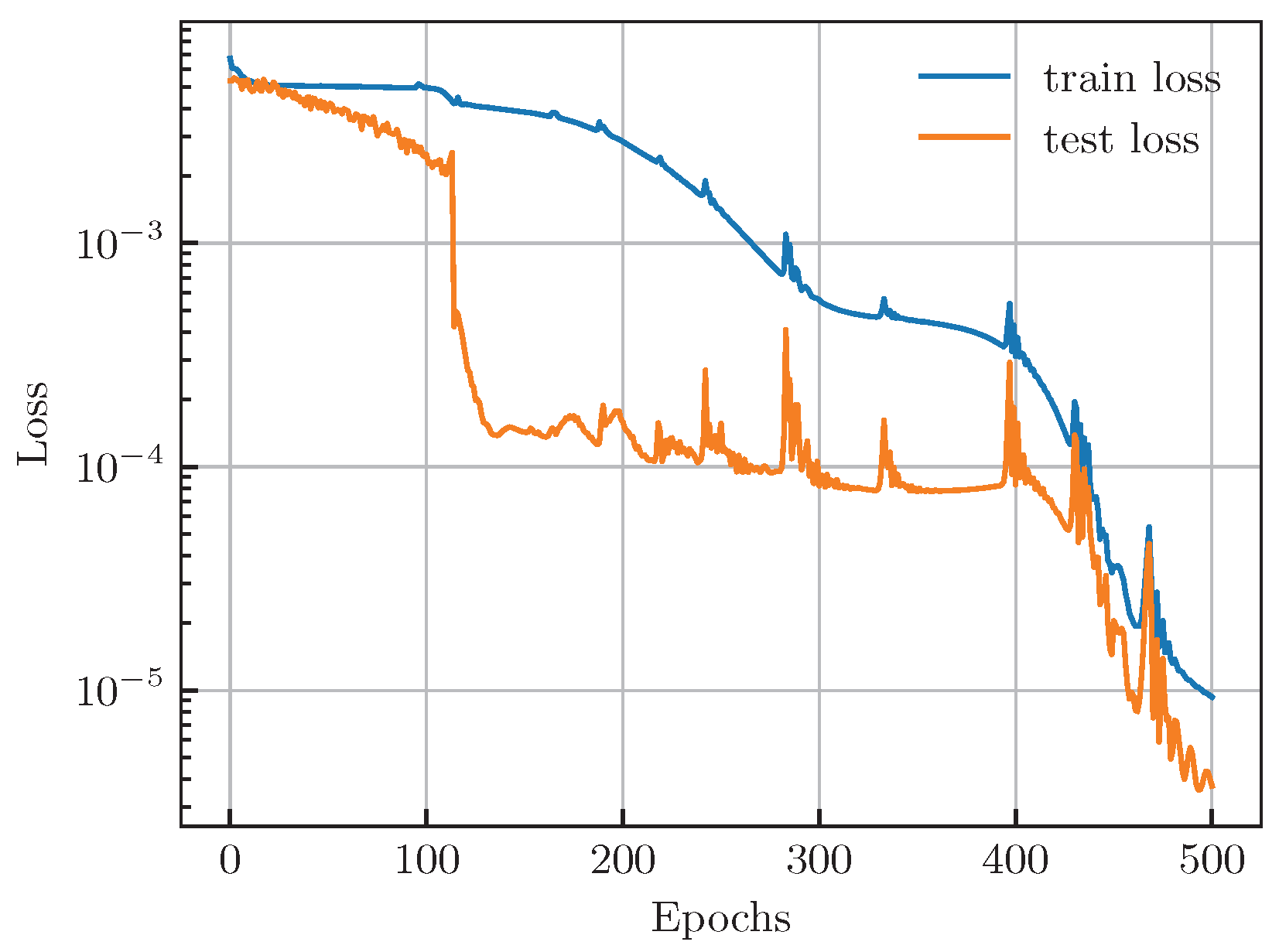Figure 5 shows the variation of the loss on the dataset during the training.

The loss on the training set decreases consistently with a more rapid decline in the final 100 epochs. At the same time, the loss on the test set remains consistently lower than that on the training set, although its trend is more complex. Starting from the 100th epoch, the test loss experiences a rapid decrease to the $1\times {10}^{-3}$ level, which is followed by almost constant maintenance with intense fluctuations over the next 250 epochs. Nonetheless, during the final 100 epochs, the test loss set decreases rapidly again, eventually approaching the $1\times {10}^{-6}$ level. Although the loss curve is not always smooth, the model’s loss reduces to a very low level after 500 epochs of training, indicating successful completion.

To more intuitively evaluate the training results, we generated 100 random motion trajectories of 10 s each using the same method described earlier. Next, we used the trained model to predict changes in the motion state of the vehicle from the same initial state within 10 s. It is important to note that the model has not predicted continuous trajectories beyond 0.1 s during training. As a result, this evaluation provides a better test of the model’s generalization ability.

Figure 6 shows the predicted generalized mass matrix by the trained model, where the learned elements remain nearly constant throughout the 10 s prediction. A remarkable result is the clear symmetry discovered by the network, where $M_{22}\approx M_{33}$ and $M_{55}\approx M_{66}$. This is not a trivial consequence of the model’s architecture but rather a meaningful demonstration of learning physical consistency.

Crucially, the neural network architecture imposes no prior structural constraints that would force these matrix elements to be equal; each output is parameterized and learned independently. The observed symmetry is a direct reflection of the physical properties of the REMUS 100 AUV, which, as an axisymmetric vehicle, exhibits an identical hydrodynamic response to motions in the sway and heave directions. The fact that our model autonomously discovered and internalized this fundamental physical principle purely from observing trajectory data serves as strong validation. It shows that the framework is genuinely learning the underlying system physics, distinguishing it from a simple black-box curve-fitter.

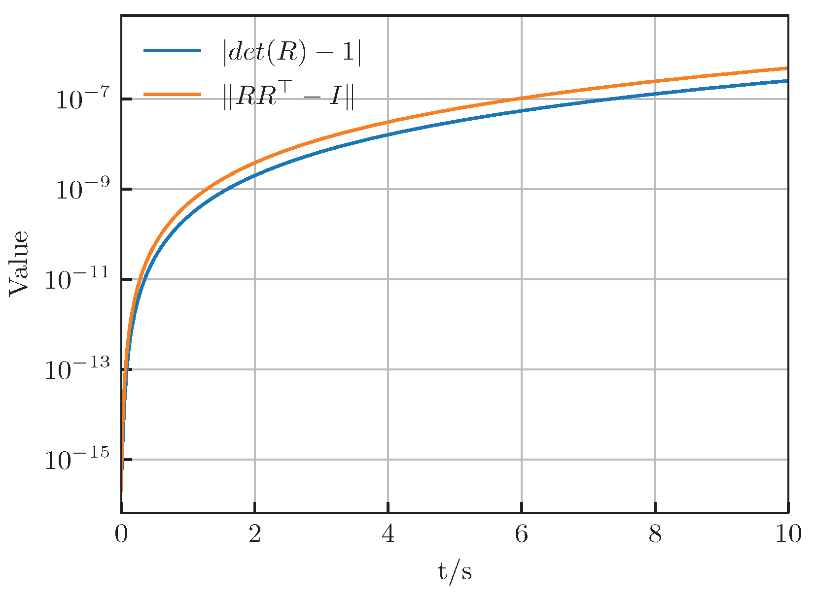
Figure 7 shows the variation of two variables associated with the rotation matrix over time, whose expected values are zero. Despite a gradual increase over time, the predicted values provided by the Hamiltonian neural network remain small with their absolute value peaking at around $1\times {10}^{-7}$. Therefore, it can be concluded that these values stay within a certain range. Our proposed method based on the Hamiltonian neural network does not rely on complex physical priors and parameter estimation, as opposed to traditional modeling methods based on differential equations. Despite its relatively simple structure, it efficiently captures the dynamic characteristics of underwater vehicles. Furthermore, the high accuracy in predicting rotational motion in the long term is still evident, which will be further demonstrated in subsequent case studies.

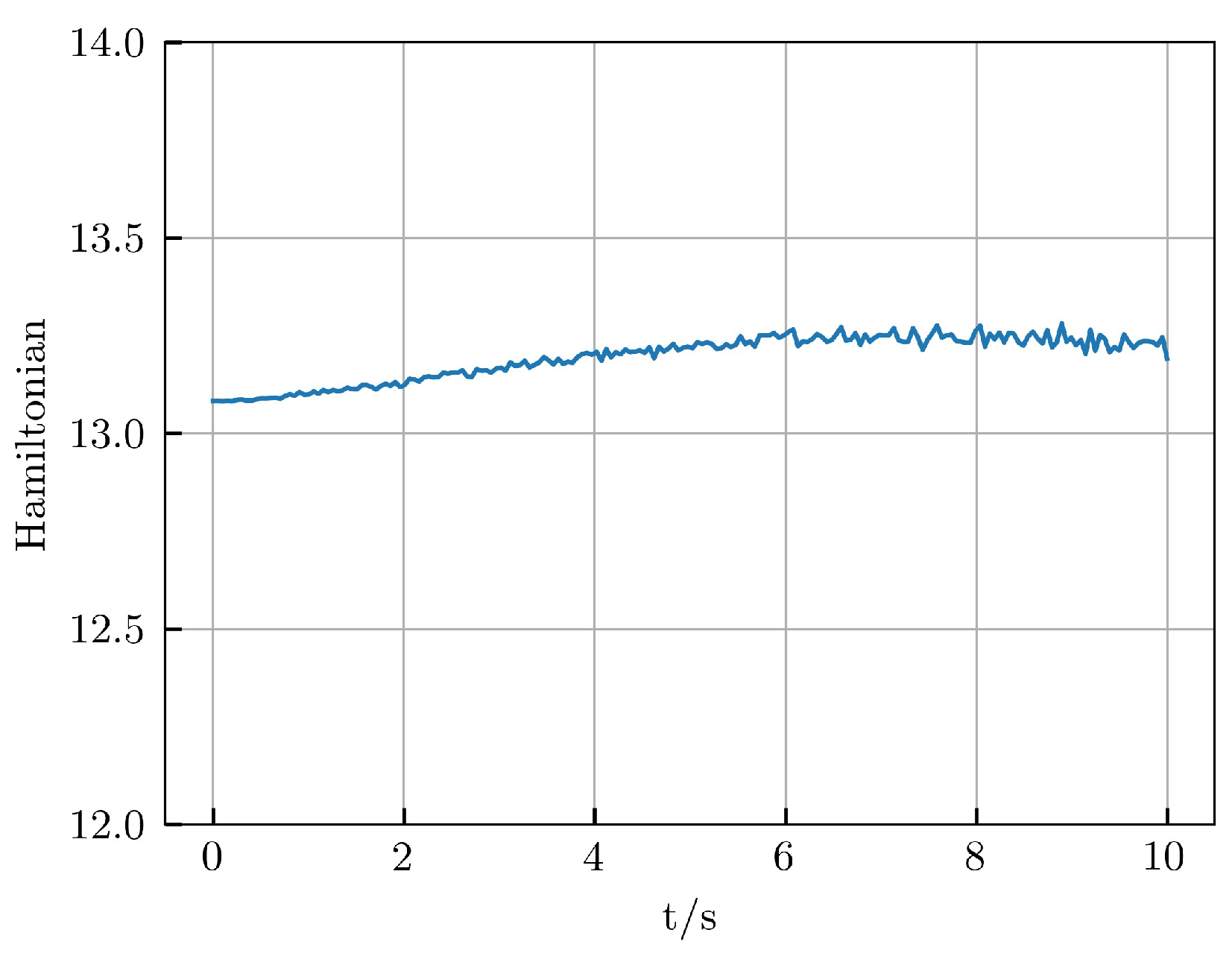
Figure 8 shows the predicted changes in the Hamiltonian over time. The Hamiltonian is not constant in this case; however, its fluctuations are very small. This implies that the model has learned the Hamiltonian’s invariance. With increasing prediction time, these fluctuations become larger, although they still remain confined to a very narrow range overall. This observation demonstrates that predicting the long-term motion of underwater vehicles is a challenging task, as errors tend to accumulate over time.

4.3. Case Study

This section presents a comparison between our HNN method and another one based on temporal convolutional networks (TCNs) [36]. The TCN takes as input the historical motion state information of the underwater vehicle over a certain time window. It employs multiple layers of temporal convolutional operations to compress the high-dimensional input, extracting effective low-dimensional features in chronological order. The extracted features are passed through several fully connected layers with nonlinear activation functions to produce the acceleration information for the current moment. The TCN has a simpler structure than our HNN. However, after extensive training with a massive amount of data, it can also demonstrate strong performance. We trained the TCN using the dataset mentioned earlier and implemented it according to the guidelines presented in [36].

4.3.1. Simple Scenarios

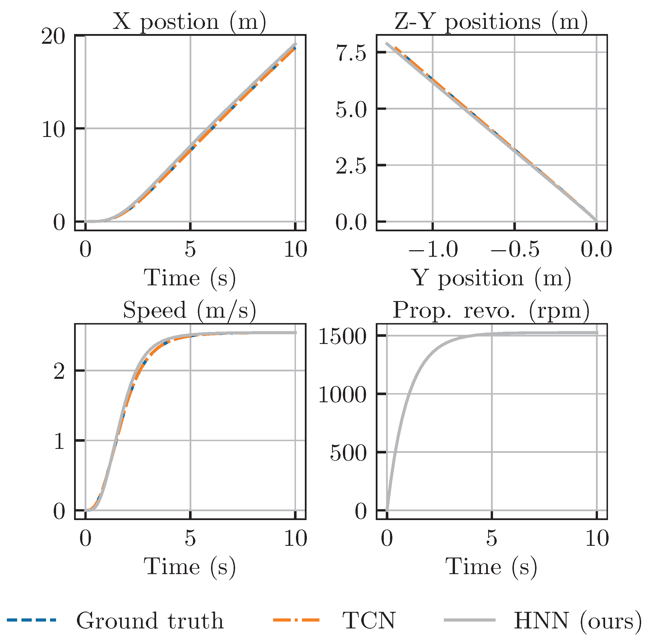
Figure 9 shows how the TCN and HNN perform when predicting the straight-line motion of underwater vehicles. In this scenario, the rudder angles for both yaw and pitch are held steady at 0 degrees, while the propeller’s rotational speed gradually increases to 1500 rpm. Both neural network-based methods effectively simulate the vehicle’s motion with predictions of remarkably similar precision. The accuracy of the TCN slightly surpasses that of the HNN. Notably, due to the coupling effects of motion, the vehicle does not strictly move in a straight line along the inertial X-axis. Instead, it exhibits slight deviations in the Y and Z-axis directions, which stabilize over time.

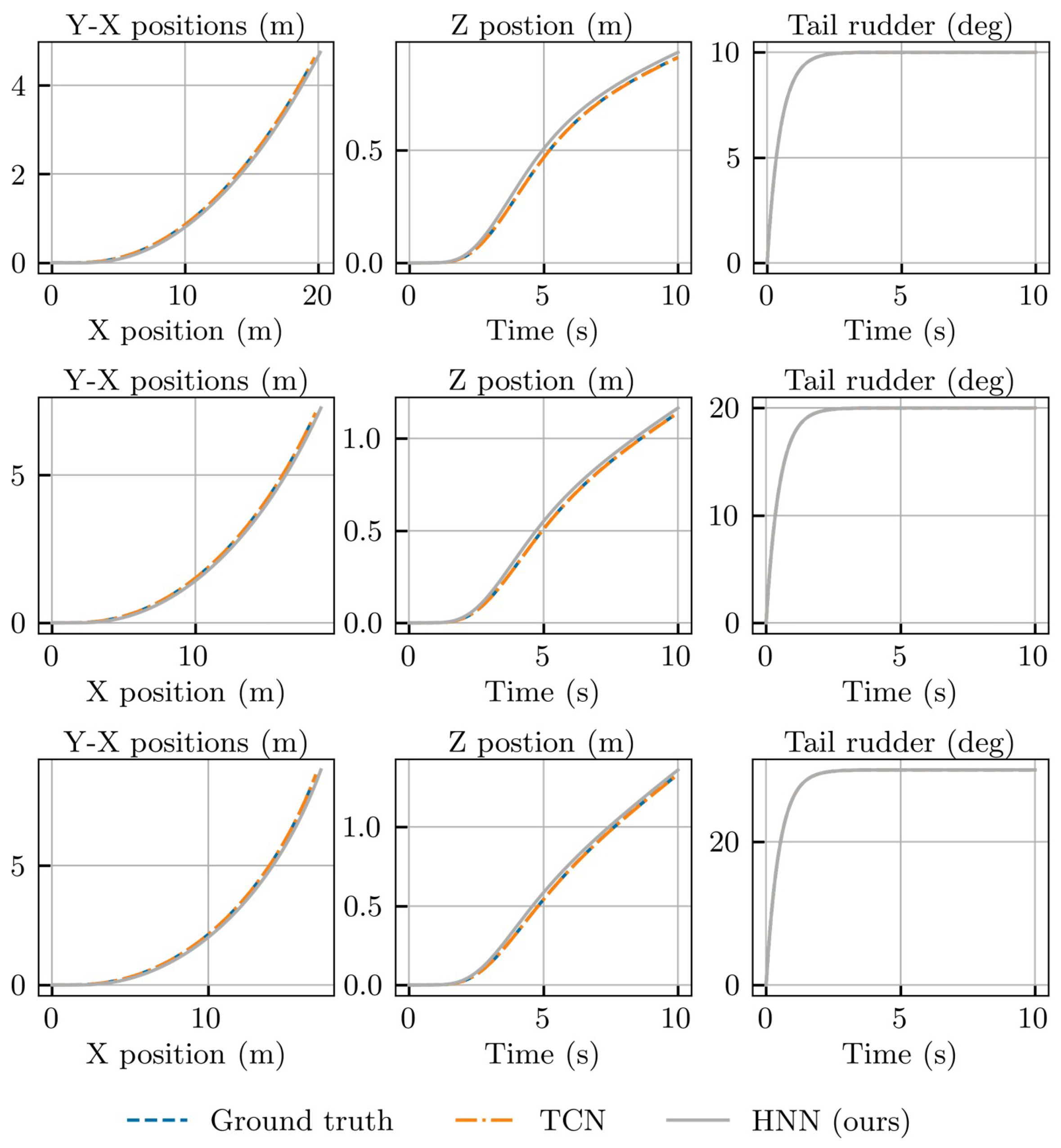
Figure 10 shows the variation in the motion state of the underwater vehicle after it is steered 10, 20, and 30 degree to the right while maintaining a propeller speed of 1500 rpm. The initial two columns depict the positional changes of the vehicle over time, and the third column demonstrates the variations in the yaw angle. The predictive outcomes of both neural network-based methods are almost identical. This suggests that both the TCN and HNN are skilled in anticipating the vehicle’s turning motion, thereby upholding a high degree of predictive accuracy, even in intricate scenarios.

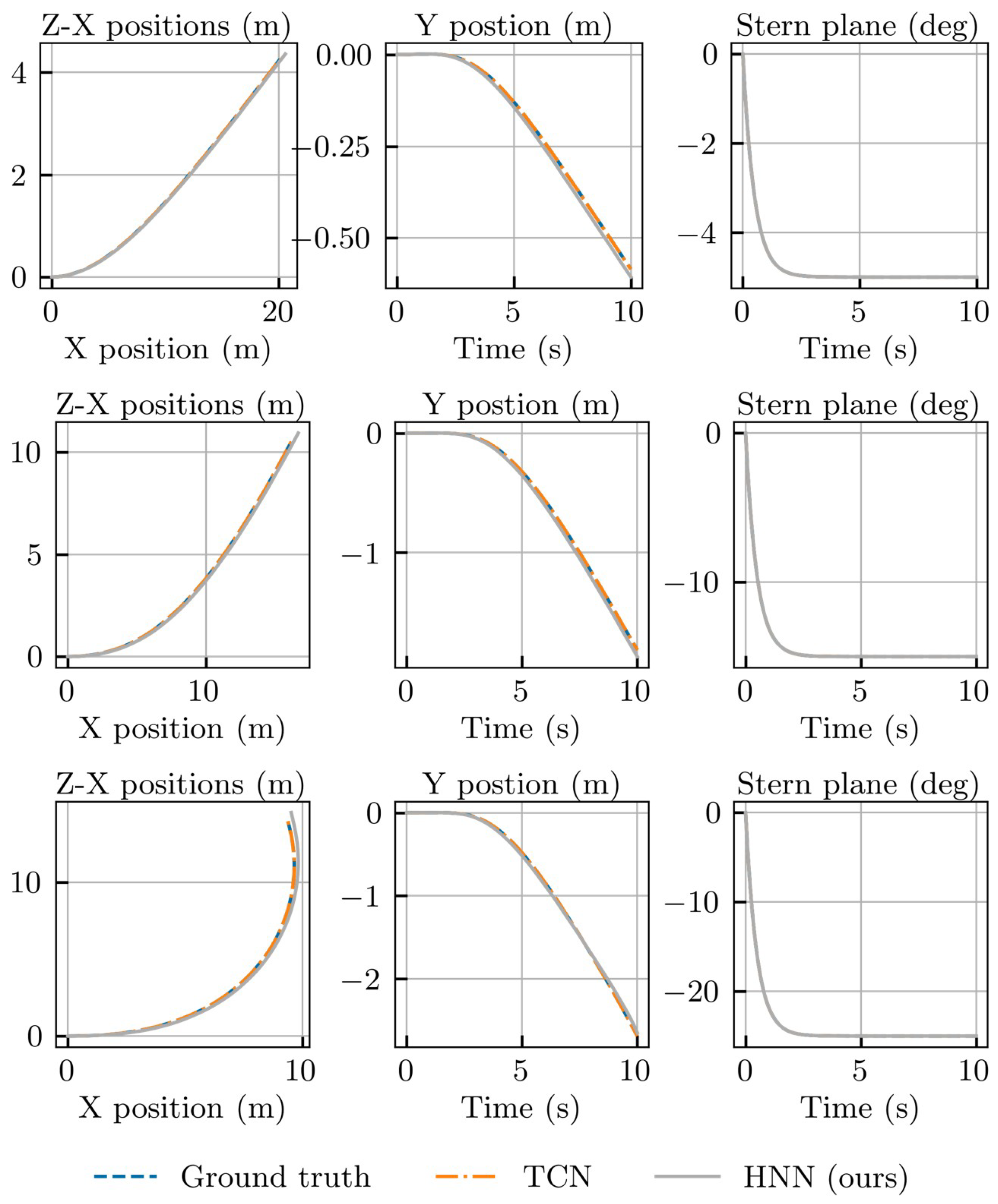
Figure 11 illustrates the motion of the underwater vehicle as the pitch angle is adjusted by 5, 10, and 15 degrees while maintaining a constant propeller speed of 1500 rpm. The vehicle initiates a descent in this scenario. The first two columns display the temporal evolution of the vehicle’s position, and the third column demonstrates the changes in the pitch angle. Both methods adeptly model the descent motion of the underwater vehicle with predictive outcomes closely aligning with benchmark data.

4.3.2. Complex Scenarios

The above analysis shows that the TCN method performs exceptionally well in simple scenarios with straight-line and turning motions even in the absence of physical priors. However, to demonstrate the benefits of the proposed HNN method, we analyze more complex motion scenarios.

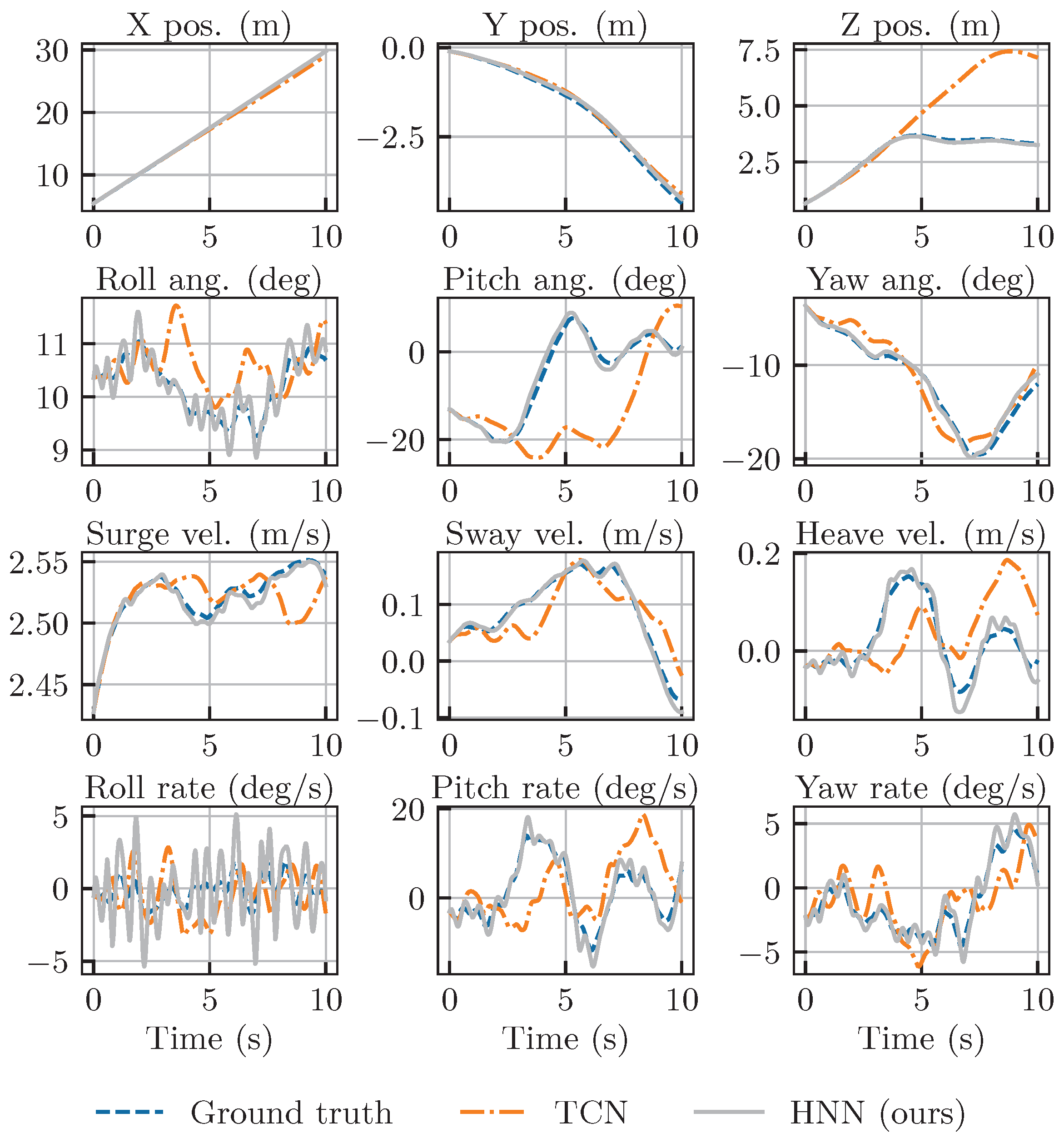
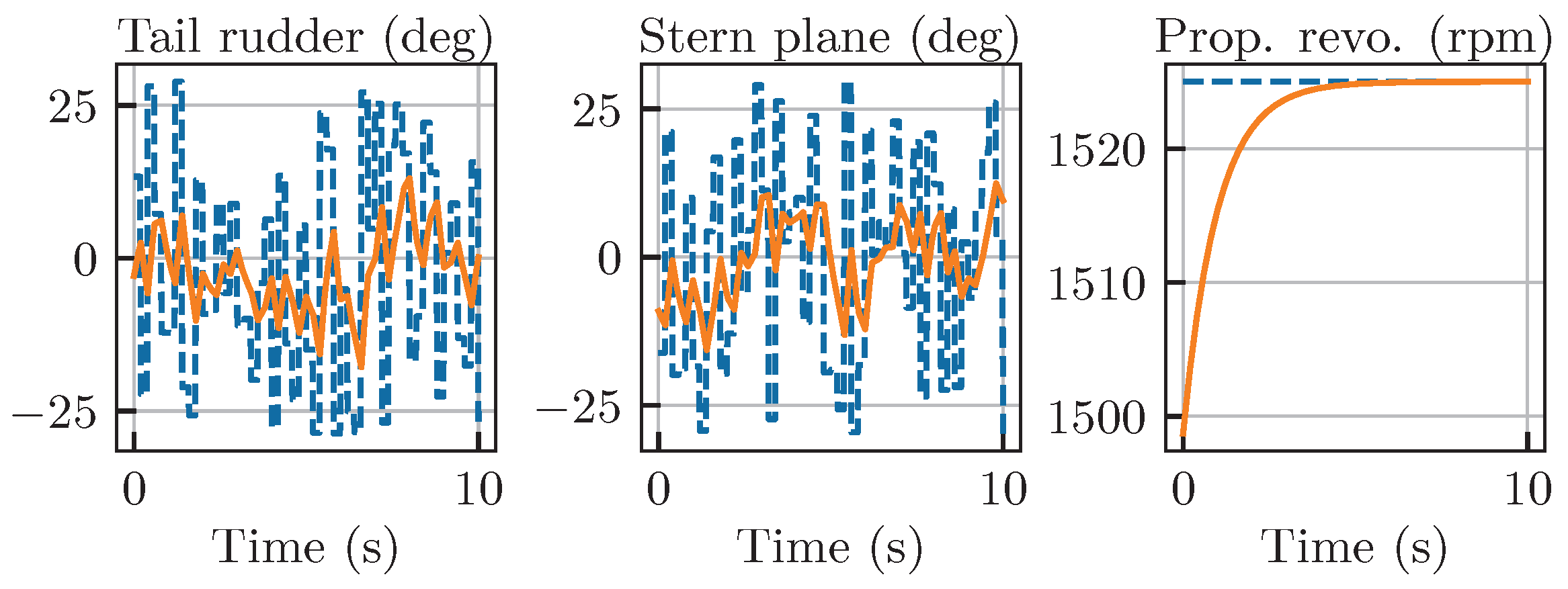
Figure 12 shows the changes in the motion state of the underwater vehicle due to random controls. The first two rows demonstrate the vehicle’s orientation in three-dimensional space, and the following two rows show the variations in velocity and angular velocity over time. Figure 13 shows the control inputs corresponding to Figure 12, where dashed lines represent desired control generated randomly, and solid lines represent the applied inputs.

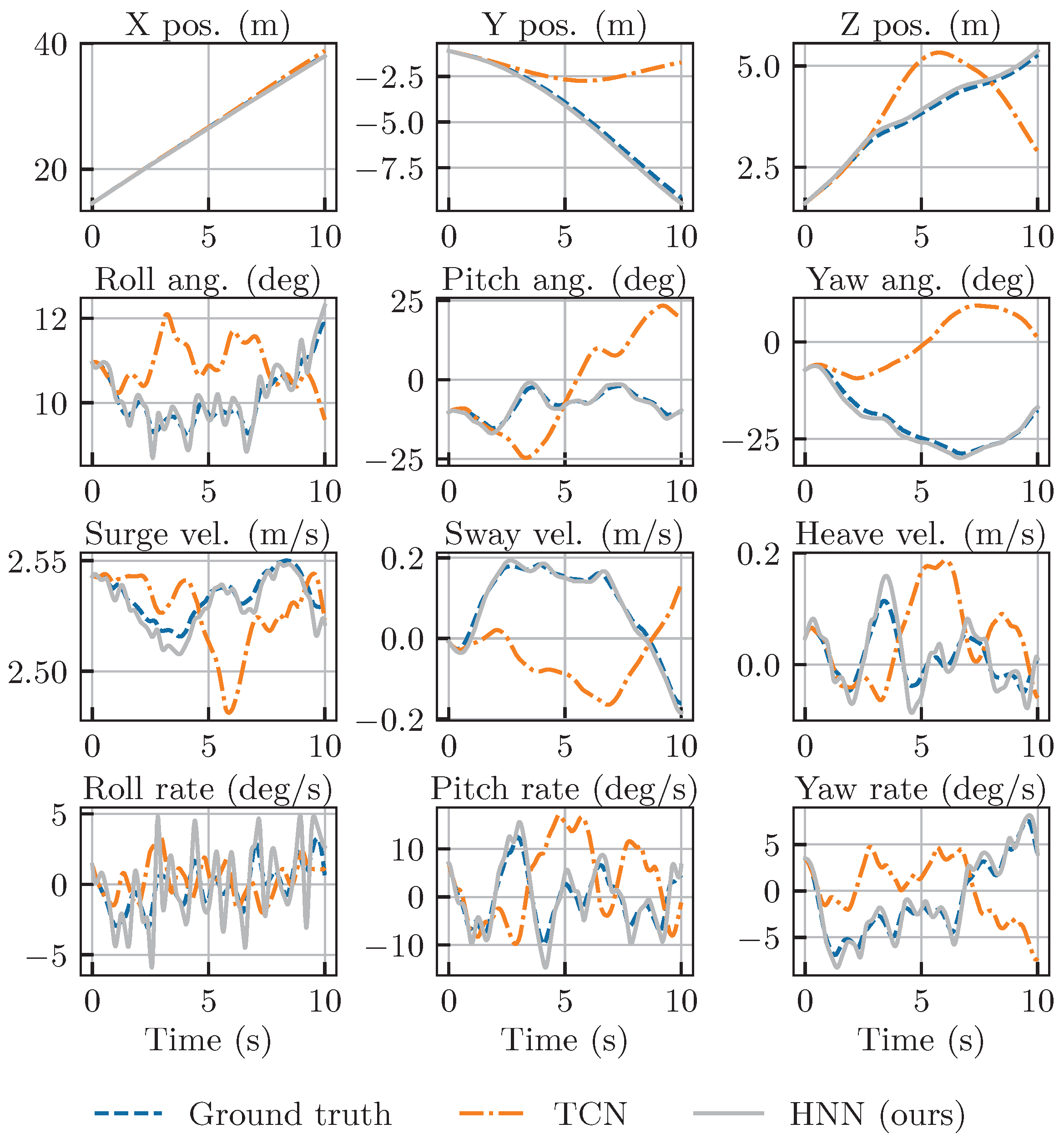
As the complexity of the control inputs increases, the TCN method maintains relatively accurate predictions of the motion of the underwater vehicle for a short time. However, approximately 2 s after the initiation of motion, TCN’s predictions of velocity vectors other than the longitudinal velocity start to deviate from the benchmark. This results in a gradual difference between the predicted and the actual motion of the vehicle. It is important to note that the TCN method demonstrated exceptional performance in the simple motion scenarios that came before.

Although the HNN method did not demonstrate superior performance to the TCN in previous scenarios, it now outperforms the TCN’s performance in the more complex control scenario. In spite of HNN’s minor overestimation in predicting the vehicle’s velocity, it consistently delivers highly accurate predictions of the vehicle’s pose that closely match the actual outcomes. This emphasizes that the HNN-based motion modeling approach, which is based on robust physical principles, better captures the dynamic characteristics of underwater vehicles, going beyond mere data fitting. The HNN method maintains consistent predictive accuracy across a spectrum of control inputs that range from simple to complex.

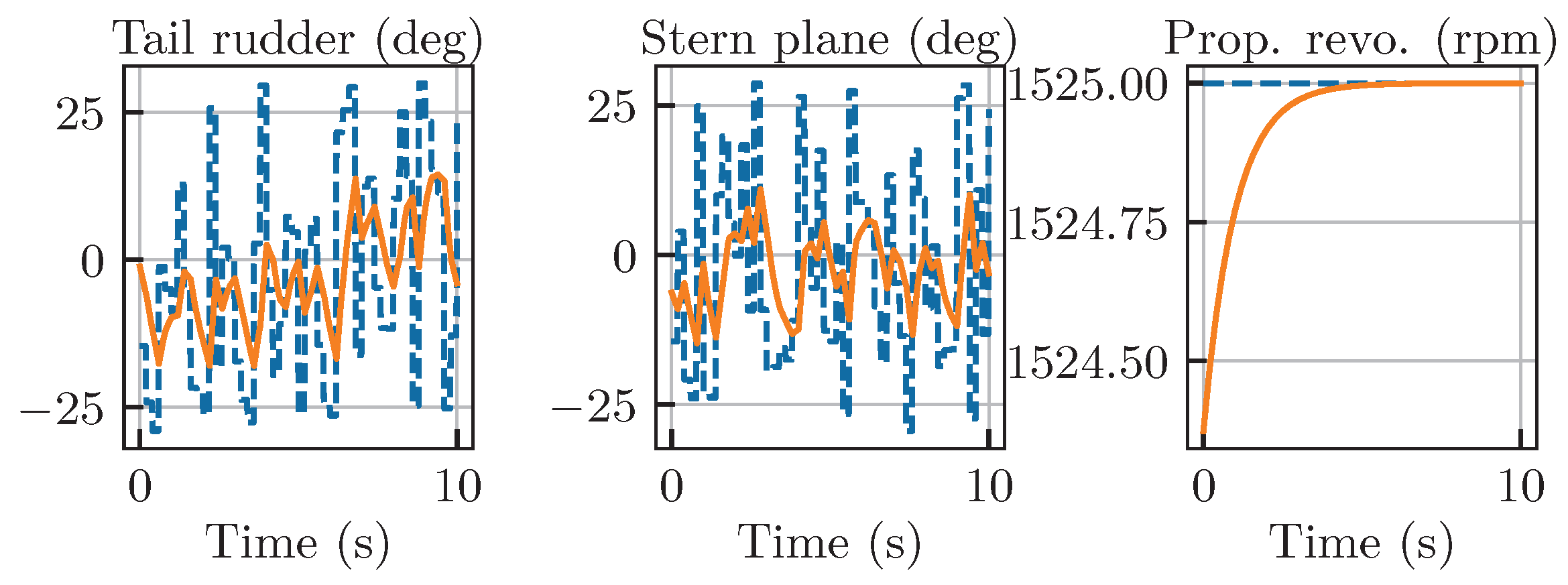
Figure 14, Figure 15, Figure 16 and Figure 17 show the motion variation in response to two additional sets of random control inputs. The TCN method maintains high accuracy only during the initial stages of motion, which is followed by a sharp decline in performance. In contrast, our HNN maintains high accuracy consistently and produces predictive outcomes that closely match the true motion. It is worth noting that both the TCN and HNN provide relatively accurate predictions of the longitudinal motion of the underwater vehicle. This is attributed to underwater vehicles such as REMUS 100, which have torpedo-like profiles and predominantly move longitudinally, accounting for a considerable part of all motion components. Through extensive data training, the TCN method is also capable of capturing this leading motion pattern. However, the proposed HNN method, which is built on the physical principles of underwater vehicle motion, consistently performs well in predicting all motion components. Therefore, the HNN outperforms in various scenarios.

While the trajectory plots in Figure 14, Figure 15, Figure 16 and Figure 17 provide a compelling qualitative illustration of the HNN’s superior robustness, a quantitative analysis is necessary to rigorously assess the performance gap between the two models. To this end, we conducted a series of 10 tests using unique, randomly generated complex control inputs, mirroring the conditions in the qualitative examples. In each test, we evaluated the 10 s prediction performance of both the HNN and TCN models against the ground truth. The root mean square error (RMSE) was calculated across the entire trajectory for key state variables.

The aggregated results of this analysis are presented in

Table 2. Quantitative comparison of 10 s prediction RMSE for HNN and TCN models, aggregated over 10 different complex random control scenarios. Values are presented as mean ± standard deviation.

Metric	HNN (Ours) (Mean ± Std Dev)	TCN (Mean ± Std Dev)
Position [m]	$0.033\pm 0.012$	$5.419\pm 0.026$
Attitude [deg]	$0.490\pm 0.169$	$5.999\pm 1.842$
Linear Velocity [m/s]	$0.007\pm 0.002$	$0.141\pm 0.005$
Angular Velocity [deg/s]	$0.659\pm 0.128$	$4.771\pm 0.678$

. The data reveal a dramatic and unambiguous difference in performance. The HNN model consistently achieves extremely low prediction errors across all metrics, with a mean position error of only 3.3 cm and very low variance, indicating its stable and reliable performance across different chaotic scenarios. In stark contrast, the TCN model’s predictions diverge significantly, resulting in a mean position error of over 5.4 m—more than 160 times greater than that of the HNN. Its errors for attitude, linear velocity, and angular velocity are also one to two orders of magnitude higher than those of our model.

This quantitative analysis provides conclusive evidence that the physics-informed structure of the HNN is essential for maintaining long-term prediction stability and accuracy when faced with complex, out-of-distribution control inputs. Under these challenging conditions, the purely data-driven TCN model, despite its strong performance in simple scenarios, proves to be unreliable and fails catastrophically.

5. Discussion

The experimental results offer a clear narrative about the differing capabilities of purely data-driven and physics-informed models, highlighting the critical distinction between interpolation and physical generalization.

5.1. The Power of Inductive Bias for Generalization

Our findings reveal a fundamental divergence in model capabilities: the TCN, as a high-capacity black-box model, excels at interpolation, whereas our HNN demonstrates superior extrapolation. The TCN’s slightly better performance in simple scenarios is a direct consequence of these test cases mirroring the constant-control structure of the training data. It is an excellent pattern-matcher for on-distribution tasks. However, this is also its critical weakness. As quantitatively demonstrated in Table 2, the TCN’s performance collapses catastrophically when faced with complex, out-of-distribution control inputs with prediction errors orders of magnitude larger than those of our HNN. This reveals the inherent brittleness of black-box models: they often learn superficial correlations rather than the underlying physical laws, making them unreliable when confronted with novel situations.

In contrast, our HNN model embodies the benefit of a strong, physically grounded inductive bias. By being architecturally constrained to adhere to the principles of Hamiltonian mechanics, it sacrifices a marginal degree of interpolative fitting capability for immense robustness and generalizability. Its ability to maintain high-fidelity predictions under chaotic conditions is its defining feature. This is powerfully evidenced by its independent discovery of the AUV’s physical symmetries ($M_{22}\approx M_{33}$ and $M_{55}\approx M_{66}$), which is a property learned purely from data rather than being hard-coded in the network architecture. This demonstrates that the model does not simply fit data; it successfully discovers the system’s fundamental laws of motion, which is the key to its robust performance.

5.2. Framework Generality and the Path to Real-World Application

It is crucial to distinguish between the implementation choices for our case study and the inherent generality of the proposed framework. The use of a simplified, predominantly diagonal structure for the learned mass and damping matrices was a deliberate engineering choice, which was justified by the well-understood, low-speed dynamics of the torpedo-shaped REMUS 100 AUV. This is not a fundamental limitation. For vehicles with more complex geometries or for high-speed regimes with strong hydrodynamic coupling, our framework can be directly configured to learn full, dense mass and damping matrices by simply adjusting the network output layers. This inherent scalability is a core strength of our methodology.

Furthermore, while this study serves as a crucial proof-of-concept within a controlled simulation environment, we recognize that bridging the “sim-to-real” gap is the ultimate objective. The current work lays the necessary foundation for this transition. Future research will proceed along a clear roadmap to address real-world complexities:

• Data-driven Robustness: We will focus on transfer learning, using the current model pre-trained on extensive simulation data as a powerful prior, and then fine tuning it on smaller, targeted datasets of real-world experimental trajectories. This strategy is expected to drastically reduce the need for expensive and time-consuming physical experiments.
• Environmental Disturbances: The Port-Hamiltonian structure can be extended to include input ports for unmodeled dynamics and external disturbances like ocean currents. Future work will investigate learning these disturbance terms or integrating the model with online estimation algorithms.
• Noise Modeling: To enhance robustness, domain randomization techniques will be applied during training, augmenting the simulation data with realistic sensor noise models (e.g., for IMUs and DVLs) to prepare the model for deployment on physical hardware.

This structured approach, built upon the validated physics-informed foundation of our current work, charts a clear course toward developing highly reliable and deployable dynamics models for real-world maritime systems.

6. Conclusions

In this paper, we introduced a novel physics-informed framework for the high-fidelity, long-term prediction of underwater vehicle dynamics by embedding Port-Hamiltonian mechanics within a neural ordinary differential equation architecture. By structurally separating energy-conserving and dissipative effects and leveraging a symplectic integrator, our model successfully learns the underlying energy landscape of the AUV directly from trajectory data. Our comprehensive experiments demonstrated that the Hamiltonian neural network (HNN) achieves exceptional robustness and accuracy, particularly under complex, chaotic control inputs where conventional black-box models like the TCN catastrophically fail. The quantitative results, revealing a performance gap of orders of magnitude, underscore the critical role of physical priors in ensuring model trustworthiness. While validated in a high-fidelity simulation, this work establishes a crucial baseline for real-world deployment. Our work provides compelling evidence that integrating physical laws is a foundational requirement for overcoming the inherent brittleness of purely data-driven methods, offering a clear path toward developing reliable, generalizable, and safe dynamic models for critical engineering systems.