Adaptive Sampling of Marine Submesoscale Features Using Gaussian Process Regression with Unmanned Platforms

Abstract

Submesoscale processes, characterized by strong vertical velocities that generate sea surface temperature (SST) fronts as well as O(1) Rossby number (Ro), are critical to ocean mixing and biogeochemical transport, yet their observation is hampered by cost and spatial limitations. Hence, this study proposes an adaptive sampling framework for unmanned surface vehicles (USVs) that integrates Gaussian process regression (GPR) with submesoscale physical characteristics for efficient, targeted sampling. Three composite-kernel GPR models are developed to predict SST, zonal velocity U, and meridional velocity V, providing predictive fields to support adaptive path planning. A robust coupled gradient indicator (CGI) is further introduced to identify SST frontal zones, where the maximum CGI values are used to select candidate waypoints. Connecting these waypoints yields adaptive paths aligned with frontal structures, while a Ro threshold (0.5–2) automatically triggers spiral-intensive sampling to collect more useful data. Simulation results show that the planned paths effectively capture SST gradient and submesoscale dynamics. The final environment reconstruction achieved the desired accuracy after model retraining, and deployment analysis informs optimal platform deployment. Overall, the proposed framework couples environmental prediction, adaptive path planning, and intelligent sampling, offering an effective strategy for advancing the observation of submesoscale ocean processes.

1. Introduction

Ocean submesoscale processes refer to ocean motions with spatial scales of O(0.1 to 10) km and temporal scales of O(0.1 to 10) days [1,2] characterized by significant vertical velocities with magnitudes of up to O(10 to 50) m/day [3] and a Rossby number (Ro)~O(1). Strong vertical velocity facilitates vertical material transports and induces pronounced sea surface temperature (SST) gradients. It is these distinctive properties that allow submesoscales to play significant roles in ocean energy cascade, material/energy transports, and air–sea interactions [4,5,6]. However, the inherent small spatiotemporal scales and rapidly evolving nature of submesoscale processes pose persistent observational challenges, which has led to a current global scarcity of observational data specifically for the submesoscale [7].

Conventional observational strategies such as ship-based transect surveys [8] or mooring observation [7] have contributed significantly to our understanding of submesoscale processes, albeit with inherent limitations. Ship-based observations are relatively costly, making prolonged implementation difficult. Furthermore, the small spatiotemporal scales of these processes make regular and frequent observations often infeasible. While mooring observations yield valuable time-series data, they fundamentally lack spatial representativeness of submesoscale processes. This lack of spatiotemporal resolution may critically limit our understanding of the key physical mechanisms and environmental impacts of submesoscale processes [9]. Consequently, there is currently an urgent need for a new observational method that is low-cost, highly mobile, and capable of regular deployment.

The recent advancement of unmanned ocean observing platforms, however, presents a transformative opportunity to overcome these limitations. Platforms such as unmanned surface vehicles (USVs), underwater gliders, and wave gliders are increasingly deployed at the forefront of ocean observation [10,11,12]. Capable of long-term, routine, and mobile ocean monitoring, these platforms offer unprecedented potential for ocean observation. Preliminary studies have demonstrated the substantial promise of unmanned platforms. For instance, Belkin et al. developed and tested a new front-tracking algorithm using an underwater glider [13]; however, their method relied heavily on substantial prior knowledge. Similarly, wave gliders have been leveraged for effective observations during typhoons [14], although they typically lack independent decision-making capabilities and require human intervention. These examples underscore the platform’s potential, yet they also highlight a common dependency on extensive prior knowledge or human intervention, pointing to the need for more intelligent and autonomous sampling strategies.

To fully leverage the potential of these platforms, the critical challenge lies in developing adaptive sampling algorithms tailored to their inherent characteristics. Existing research has explored such strategies for specific phenomena. For example, Woithe et al. proposed and validated an adaptive thermocline-tracking algorithm for AUVs, which can reduce energy consumption by over 50% by activating sensors only in response to specific conditions [15]. Zhang et al. developed an automatic detection and tracking algorithm for coastal upwelling fronts based on vertical temperature differences and validated it with AUV experiments in Monterey Bay [16]. Furthermore, Petillo et al. defined frontal positions using isotherms, developing an adaptive tracking algorithm and successfully demonstrating its feasibility for online identification and tracking via AUV simulations [17]. While these studies demonstrate a high degree of automation in target detection and tracking, they are primarily focused on larger or more persistent oceanographic features. Consequently, the adaptive sampling of rapidly evolving submesoscale processes remains an open challenge. Addressing this challenge for submesoscale processes requires a probabilistic modeling approach that can efficiently learn and predict the spatial structure of the environment with limited data. Gaussian process regression (GPR) is ideally suited for this task.

Prior knowledge of the spatial characteristics of the target area is essential for adaptive decision making in ocean observation. GPR effectively addresses this need. As a lightweight yet powerful machine learning model [18], GPR has been widely used for spatial field modeling and prediction [19,20]. It is particularly valuable in developing adaptive observation algorithms, as it can provide reliable environmental predictions even when prior data are limited or unavailable.

Several studies have demonstrated the feasibility of GPR-based adaptive sampling. Kai-Chieh Ma utilized mutual information derived from GPR-predicted spatial fields for online path planning, enabling an autonomous surface vehicle (ASV) to maximize information acquisition during lake exploration [20]. Similarly, Fossum et al. developed an uncertainty function combining prediction variance and spatial gradient within a GPR framework, applying it to adaptive thermocline sampling with experimental validation [21]. While these studies establish the utility of GPR in adaptive observation, they do not systematically address the critical selection of kernel functions to optimize predictive accuracy. Motivated by this gap, our study systematically evaluates multiple kernel configurations to enhance model performance, thereby tailoring the GPR-based adaptive observation framework specifically for complex submesoscale processes.

Targeting complex submesoscale processes, we propose an adaptive sampling framework for USVs that integrates GPR with submesoscale physical characteristics. The approach develops three composite-kernel GPR models to predict SST, zonal velocity (U), and meridional velocity (V), generating predictive fields to guide path planning. A robust coupled gradient indicator (CGI) is introduced to identify SST frontal zones, with maximum CGI values used to select candidate waypoints. Connecting these waypoints produces adaptive paths aligned with frontal structures, while a Rossby number threshold (0.5–2) automatically triggers spiral-intensive sampling around selected waypoints to enhance data acquisition.

The remaining sections of the paper are organized as follows: Section 2 of this article introduces the data utilized and the research framework. Section 3 primarily presents the adaptive sampling results of the submesoscale. Section 4 discusses the simulation findings and shortcomings, and Section 5 summarizes the key conclusions and outlines the planned next steps.

2. Materials and Methods

2.1. Data and Study Area

The data used in this study were obtained from the Massachusetts Institute of Technology General Circulation Model (MITgcm), specifically the LLC4320 dataset. This dataset features a high horizontal resolution of 1/48°, 90 vertical layers, and hourly temporal sampling, covering the period from September 2011 to November 2012. Having been widely used in submesoscale studies [9,22,23,24,25], and validated for its reliability in simulating submesoscale processes, the LLC4320 data are treated as ground truth in this work. Within this simulated marine environment, the uniform motion of a USV was simulated, and observational data were collected using a fixed sampling protocol. These data were subsequently used to develop a GPR-based submesoscale adaptive sampling algorithm.

To enable comprehensive analysis and comparative evaluation, three study regions (A1, A2, and A3, see Figure 1) were selected based on their differing levels of submesoscale activity, as illustrated in Figure 2. This study focuses on the primary variables of SST and horizontal velocity components (U, V), with data sourced from specific snapshots: 2012-06-28T01:00 UTC for regions A1 and A2 and 2012-07-01T13:00 UTC for region A3.

To remove tidal and inertial signals, a fourth-order Butterworth low-pass filter with a cutoff period of 36 h was applied to the LLC4320 dataset [3]. The filtered results are presented in Figure 2, where the three columns correspond to study areas A1, A2, and A3, respectively. The first row displays the SST distribution, the second row shows the Ro field, and the third row illustrates the strain rate distribution. These three fields exhibit a notable degree of spatial correspondence, with active submesoscale regions characterized by pronounced SST gradients and elevated strain rates.

2.2. Gaussian Process Regression Modeling

GPR is a non-parametric probabilistic model based on the Bayesian framework. Its core concept relies on Gaussian processes to describe the prior distribution of the target function, which is then updated to a posterior distribution using observed data. By employing kernel functions to model spatial correlations, GPR enables effective prediction of spatial fields [19,20,26]. This method is characterized by strong generalization capability, simple model training, self-adapting hyper-parameters, interpretability, and robustness [27,28]. It is particularly well suited for addressing spatial regression problems involving non-linearity, high dimensionality, and small-sample data [18]. The predictive performance of GPR depends primarily on the choice of the covariance function (kernel function), which governs the model’s ability to capture underlying data structures [18].

Assume the target function $f:R^D\to R$ follows a Gaussian process, with its prior distribution expressed as:

$$f(x)~GP(m(x),k(x^{\prime }))$$

(1)

where:

• $m(x)$: Mean function, describing the global trend of the function. For the purposes of simplification, the mean function is typically taken to be 0 [19].
• $k(x,x^{\prime })$: Kernel function, governing the local behavior of the function.
• $x$ and $x^{\prime }$ represent any two spatial data.

The selection of the kernel function plays a crucial role in determining the predictive accuracy and reconstruction capability of the GPR model. Since individual kernel functions often exhibit limited flexibility when modeling complex systems, this study employs combined kernel functions. Previous work has established that valid kernel functions can be constructed through the sum, product, or scaling of existing kernels [18].

Four commonly used kernel functions were selected as base components: Linear, Radial Basis Function (RBF), Matérn32, and Exponential. The RBF kernel—also referred to as the squared exponential (SE)—is among the most widely used; it is infinitely differentiable, yielding Gaussian processes with mean-square derivatives of all orders and consequently very smooth response surfaces. However, this smoothness may limit its ability to capture abrupt variations [18]. The Linear kernel is suitable for data exhibiting dominant linear trends. In contrast, the Matérn kernel family offers greater flexibility through its shape parameter $\mathrm{v}$, which typically takes values such as 1/2, 3/2, or 5/2. Smaller values of $\mathrm{v}$ enhance the kernel’s ability to model non-smooth processes, making it particularly advantageous for oceanic and meteorological applications. Notably, when $\mathrm{v}$ = 1/2, the Matérn kernel simplifies to the Exponential kernel [18,28].

By combining different kernel functions, the model can adapt to a wider range of data variations. Each kernel quantifies similarity between spatial points using hyper-parameters such as length scale and signal variance, which are typically optimized via marginal likelihood maximization (MLM) [18].

Formally, let $X$ denote a set of n training points associated with target values $\mathrm{y}$, and $X_{*}$ represent test points. When observation noise is not considered, the prediction equations for GPR can be summarized as:

$$\left.f_{*}\right|X,y,X_{\ast }~N\left(\overline{f_{*}},cov\left(f_{*}\right)\right)$$

(2)

$$\overline{f_{*}}\triangleq E\left[\left.f_{*}\right|X,y,X_{*}\right]=k\left(X_{*},X\right)k{\left(X,X\right)}^{-1}y$$

(3)

$$cov\left(f_{*}\right)=k\left(X_{*},X_{*}\right)-k\left(X_{*},X\right)k{\left(X,X\right)}^{-1}k\left(X,X_{*}\right)$$

(4)

Taking the Matérn kernel as an example, its mathematical expression is as follows:

$$k\left(x,x^{\prime }\right)={\sigma }_f^2{\displaystyle \frac{2^{1-v}}{\mathrm{\Gamma }\left(v\right)}}{({\displaystyle \frac{\sqrt{2v}\parallel x-x^{\prime }\parallel }{l}})}^v{K}_v({\displaystyle \frac{\sqrt{2v}\parallel x-x^{\prime }\parallel }{l}})$$

(5)

where ${\sigma }_f^2$ denotes the signal variance, l is a length-scale hyper-parameter, $K_v$ is a modified Bessel function, and $\mathrm{\Gamma }$ is a gamma function. Assigning $v$ = 2/3 yields the Matérn32 kernel function.

Let $\theta =\{{\sigma }_f^2,l\}$ denote the set of hyper-parameters of the kernel function. The appropriate selection of $\theta$ enables the kernel function to accurately characterize the data distribution and underlying physical phenomena. A widely adopted optimization method is marginal likelihood maximization (MLM), which determines the optimal hyper-parameters by maximizing the model’s log-marginal likelihood function. The mathematical expression is given as follows:

$$L\left(\theta \right)=argmax logp\left(y|X|,\theta \right)={\displaystyle \sum _{i=1}^n\ln p\left(y_i|x_i,\theta \right)}$$

(6)

The hyper-parameters of the composite kernels are optimized by maximizing the log-marginal likelihood given in Equation (6). The initial values are set heuristically to facilitate stable convergence: the signal variance ${\sigma }_f^2$ for each kernel is initialized to the variance of the training target values $y$, while the initial length scales $l$ are set to the mean of the variances across each dimension of the input coordinate data. Optimization is performed using the L-BFGS-B algorithm, a quasi-Newton method. This optimizer was selected for its computational efficiency and robust convergence properties, which well-match the characteristics of our model. The convergence criteria are defined by a gradient tolerance of gtol =1 × 10⁻⁶ and a parameter change tolerance of xtol = 1 × 10⁻⁶, with a maximum of 1000 iterations permitted to ensure a balance between computational efficiency and solution accuracy. No fixed random seed was set.

In this work, we use a composite kernel, which is a function formed by combining base kernels through addition or multiplication. The adopted form is defined as Equation (7), and this additive structure was chosen based on the hypothesis that different components of the signal (e.g., SST) influence the system response in an independent and additive manner. Following previous research, the weighting coefficients $w_1$ and $w_2$ are fixed at 1.0 [28], an approach taken to maintain model simplicity and mitigate overfitting.

$$k\_composite\left(x, x^{\prime }\right)=w_1\cdot k_1\left(x, x^{\prime }; {\theta }_1\right)+w_2\cdot k_2\left(x, x^{\prime }; {\theta }_2\right)$$

(7)

It should be supplemented that all experiments were conducted on a computer equipped (Tongfang Co., Ltd, Shanghai, China) with an Intel Core i7-9750H CPU (6 cores, 2.60 GHz), 32 GB of RAM, and an NVIDIA GeForce GTX 1660 Ti GPU with 6 GB of memory. The operating system was Windows 10, and the GPy version used was 1.10.0.

2.3. Multilayer Perceptron Model

The multilayer perceptron (MLP), as a classical feedforward neural network model, typically consists of an input layer, one or more hidden layers, and an output layer. Its fundamental principle relies on adjusting the connection weights and transfer functions (activation functions) between layers, enabling the network to approximate arbitrarily complex non-linear mappings through learning. According to the Universal Approximation Theorem by Hornik et al. [29], given sufficient neurons in the hidden layer and appropriate weight configurations, an MLP can approximate any smooth, measurable input-output functional relationship to arbitrary precision.

Based on MLP, the functional relationship between input and output vectors can be established,

$$y=f(x)$$

where the input matrix $x$ has dimensions [n, k], n represents the number of training patterns, and k denotes the number of input nodes/variables. Similarly, the output matrix $y$ has dimensions [n, j], where j indicates the number of output nodes/variables.

In this study, we constructed an MLP model with two hidden layers comprising 22 and 11 neurons, respectively. The ReLU activation function was employed in the hidden layers to introduce non-linearity. The model was trained using the backpropagation algorithm with the Adam optimizer, and an early stopping strategy was adopted to prevent overfitting. The input data were normalized to zero mean and unit variance before training and the mean squared error was used as the loss function.

We built the MLP model using the MLPRegressor class from the scikit-learn library (version 1.3.2), while keeping all other hardware configuration conditions unchanged.

2.4. Adaptive Sampling Framework

Based on the environmental predictions, the GPR-based adaptive sampling framework is structured around three key modules: frontal identification, achieved through the CGI to effectively target SST fronts; adaptive path planning, which exploits predictive environmental fields to optimize waypoint selection; and intensive sampling, triggered by Ro thresholds to capture fine-scale variability. The subsequent sections elaborate on the design and implementation of these modules, highlighting how their integration ensures efficient and targeted USV observations of submesoscale.

2.4.1. Frontal Identification Using the Coupled Gradient Indicator

An oceanic front, marking the boundary between distinct water masses, manifests as a zone of strong gradients. However, the SST field is complex, and gradient magnitudes are spatially heterogeneous; significant changes are not always present in a given local area. This poses a challenge for traditional methods that rely solely on local SST gradient maxima, as they can cause a USV to become trapped in local extrema, failing to capture the frontal structure. Since fronts are a primary surface manifestation of submesoscale processes, their accurate identification is a crucial prerequisite for targeted observation.

The spatial heterogeneity of SST gradients is not random but is dynamically linked to kinematic properties. As illustrated in Figure 2, these gradients exhibit a strong correspondence with regions of elevated Ro and strain rate, suggesting a coupling between thermal fronts and velocity field dynamics. This coupling is statistically supported by positive Pearson correlation coefficients between SST gradients and strain rate gradients in study regions A1, A2, and A3 (0.46, 0.44, and 0.30, respectively; p < 0.01), indicating that regions of dramatic SST variation often coincide with intense deformation of the current field, demonstrating a moderate but significant coupling between SST and dynamical gradients. This physical rationale underpins our introduction of the CGI. The CGI integrates three normalized components into a unified metric: the gradient of SST, the gradient of strain rate (Equation (9)), and the GPR-predicted variance (Equation (13)), which quantifies estimation uncertainty (Figure 3).

The CGI is formulated as the product of the magnitudes of the key gradient fields:

$$CGI=norm | | \nabla SST | | \ast norm | | \nabla D | | \ast norm(error)$$

where “norm” in the CGI definition refers to the min–max scaling operation, which normalizes each gradient field (∇SST, ∇D, error) individually to a [0, 1] range based on their respective minimum and maximum values across the computational domain. Here, the symbol ∇ denotes the spatial gradient, which is computed numerically using the central difference method via the numpy.gradient function. This step is crucial to eliminate unit differences and ensure that all three components contribute equally to the composite index.

$$‖\nabla SST‖=\sqrt{{(\partial SST/\partial x)}^2+{(\partial SST/\partial y)}^2}$$

(8)

$$‖\nabla D‖=\sqrt{{(\partial D/\partial x)}^2+{(\partial D/\partial y)}^2}$$

(9)

$$S={\displaystyle \frac{\partial U}{\partial x}}-{\displaystyle \frac{\partial V}{\partial y}}$$

(10)

$$N={\displaystyle \frac{\partial V}{\partial x}}+{\displaystyle \frac{\partial U}{\partial y}}$$

(11)

$$D=\sqrt{S^2+N^2}$$

(12)

$$error=k\left(X_{*},X_{*}\right)-k_{*}\ast K^{-1}\ast k_{*}$$

(13)

where $S$ and $N$ are the stretching and shearing terms, $D$ denotes strain rate, error denotes prediction variance in the GPR model, $k_{*}$ denotes the kernel vector between the test point $x_{*}$ and training points $\left\{x_i\right\}$.

The design of the CGI serves the initial purpose of enabling robust frontal detection. The assignment of equal weights to the three components in the CGI is a deliberate design choice, justified on three grounds. First, it creates a synergistic interplay: high values of the SST and strain-rate gradients serve as direct indicators of dynamically active submesoscale regions. The normalized prediction error complementarily guides exploration: it targets areas of high model uncertainty (often associated with complex field variation) when physical gradients are weak and mitigates over-reliance on local extremes when physical gradients are strong. Second, the preceding min–max scaling of each component to a unified [0, 1] range establishes a non-dimensional and equitable basis for this interaction. Finally, this equal-weight scheme offers a transparent, robust, and simple formulation, which has proven effective in our experiments.

The application of this composite index to the GPR-predicted fields yields a continuous scalar representation of oceanic activity. The identification logic leverages the continuous nature of the oceanic field. The GPR framework is well-suited to this task, as its predictions intrinsically account for non-linear and continuous spatial variations. Consequently, frontal structures are identified by iteratively locating the maximum of the normalized CGI across a series of search areas. This approach demonstrates the feasibility of frontal detection based on local gradients derived from GPR-predicted fields. The method ensures robust identification by responding to a coherent signal integrating both thermal and dynamical gradients, rather than reacting to potentially misleading local SST extrema.

2.4.2. Adaptive Path Planning Strategy

Adaptive path planning forms the foundation of adaptive sampling, enabling a USV with a limited sampling radius to collect meaningful data along its path. The process begins with an initial zigzag path performed by the USV to obtain preliminary field data. These observations are used to drive the GPR models, which generates predictive fields of SST, U and V for the local region, providing the necessary information for subsequent path planning.

The core of our path planning approach is a waypoint determination method that iteratively maximizes the local magnitude of the CGI. This strategy inherently prioritizes regions with the most significant and dynamically coherent gradient variations. Notably, in areas where gradients of SST and velocity are weak, the magnitude of the CGI may be primarily influenced by the gradient of the prediction variance. In such cases, path planning is effectively guided by spatial uncertainty, directing the USV to explore regions of higher model uncertainty gradient and thus contributing to adaptive data collection.

Connecting these waypoints with straight-line segments constructs an observation path that reliably traverses the most active frontal zones, avoiding diversion toward isolated gradient peaks. This path ensures effective frontal detection and prepares for subsequent sampling. When a local area satisfies the Ro threshold (indicating probable submesoscale activity), the USV is directed to execute an intensive spiral sampling pattern to enhance spatial coverage. The combination of gradient-maximizing paths and localized spiral paths jointly defines the complete adaptive sampling strategy.

It is noted that initial deployment locations significantly influence the resulting paths, as complex variations in SST and currents affect the positions of target waypoint. Therefore, the optimal selection of the starting point is a critical consideration, which is analyzed in Section 3.3.

2.4.3. Submesoscale Confirmation Based on Rossby Number Threshold

Submesoscale phenomena are typically associated with SST fronts. When the USV approaches near the SST front, it enters a region likely to exhibit submesoscale activity; however, an objective criterion is required to confirm their presence. To address this, a Ro threshold was introduced to identify submesoscale processes at the local scale.

Although substantial progress has been made in submesoscale research, the precise definition of this scale remains debated. Zheng et al. proposed a broad classification of submesoscale phenomena as processes with spatial scales of 1–100 km and Ro between 0.5 and 10 [30]. For context, the Ro of internal waves has been reported as O(2–10) when using wavelength as the horizontal length scale at 20°N [30], while the M2 internal tide exhibits a Ro on the order of O(0.5) [31]. Building on these studies, we adopted a Ro threshold range of 0.5–2. A local point was flagged as potentially submesoscale if its Ro fell within this interval. To enhance reliability, a local area was classified as actively submesoscale only if over 60% of its grid points satisfied the threshold, triggering an intensive observation strategy. While this criterion is intentionally broad, it provides a practical and effective means for automated identification of submesoscale.

The calculation formula for Ro is as follows:

$$Ro={\displaystyle \frac{\xi }{f}}$$

(14)

$$\xi ={\displaystyle \frac{\partial v}{\partial x}}-{\displaystyle \frac{\partial u}{\partial y}},f=2\omega sin\theta$$

(15)

where $\xi$ denotes relative vorticity, $f$ denotes planetary vorticity, $\omega$ denotes the angular velocity of Earth’s rotation, and $\theta$ represents latitude.

2.4.4. Integrated Implementation Workflow

We propose an effective adaptive sampling framework comprising three key components: (1) an adaptive path planning method that determines target waypoints by identifying the maximum of the CGI; (2) a frontal search method that utilizes local gradient information to infer large-scale gradient features; and (3) a feature confirmation criterion based on a Ro threshold, which triggers spiral-shaped intensive sampling when activated. It should be noted that spiral paths constitute a specialized form of path planning under the intensive sampling mode.

During frontal search, a sequence of target points is automatically generated based on the CGI to form the observation path. When submesoscale features are confirmed, an intensive observation strategy is implemented to produce denser sampling paths and acquire higher-resolution data. A schematic overview of the adaptive observation process is provided in Figure 4, and the corresponding workflow is detailed in Figure 5.

The detailed operational procedure is structured as follows:

(1)

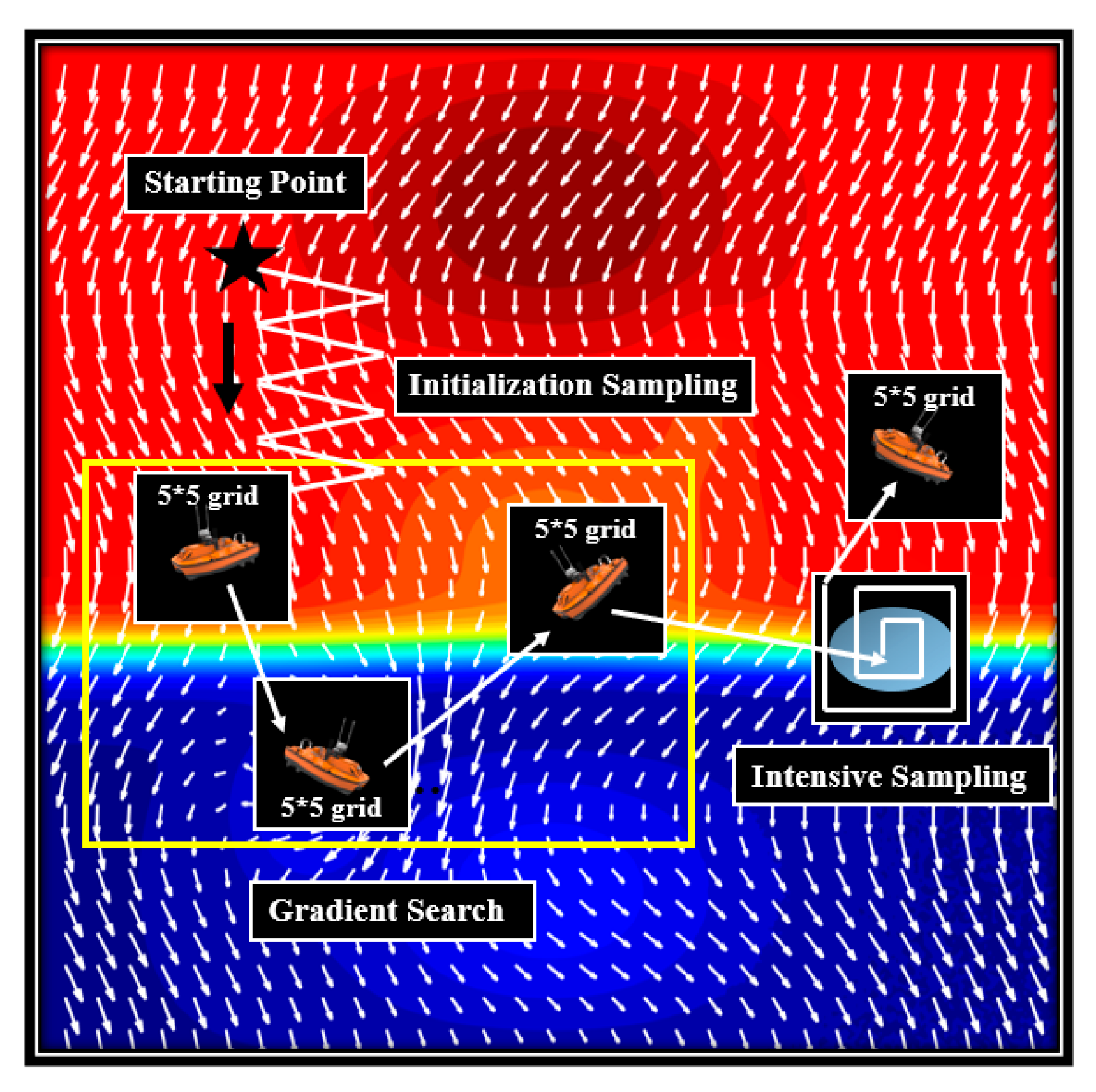
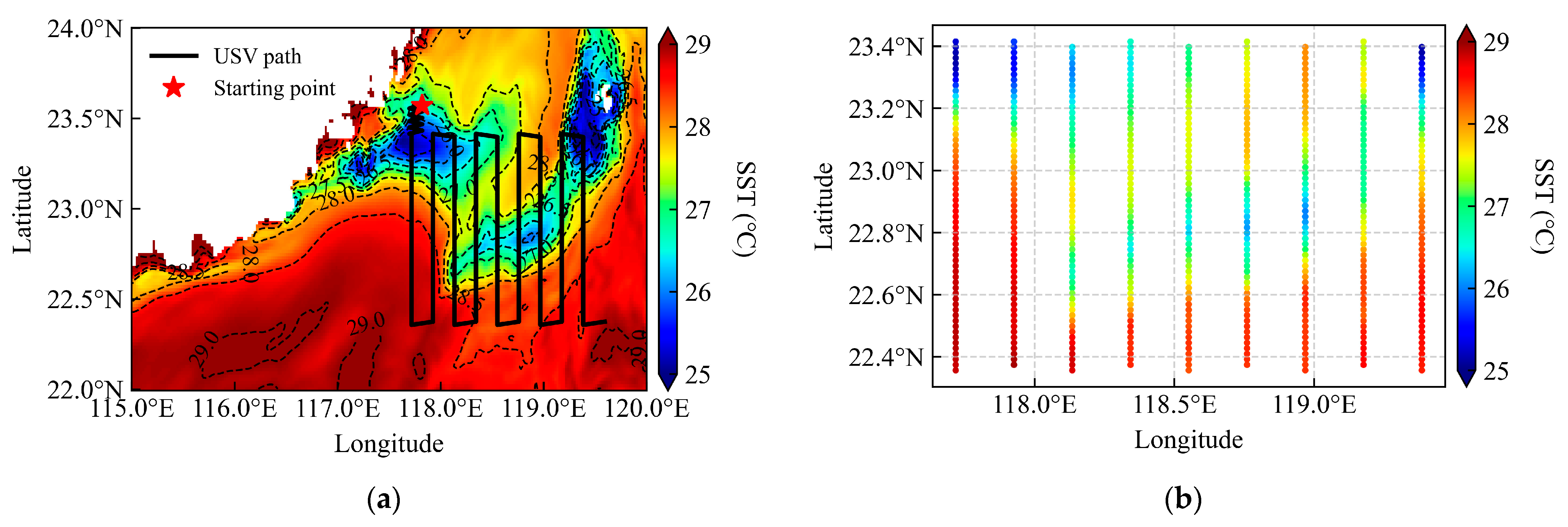
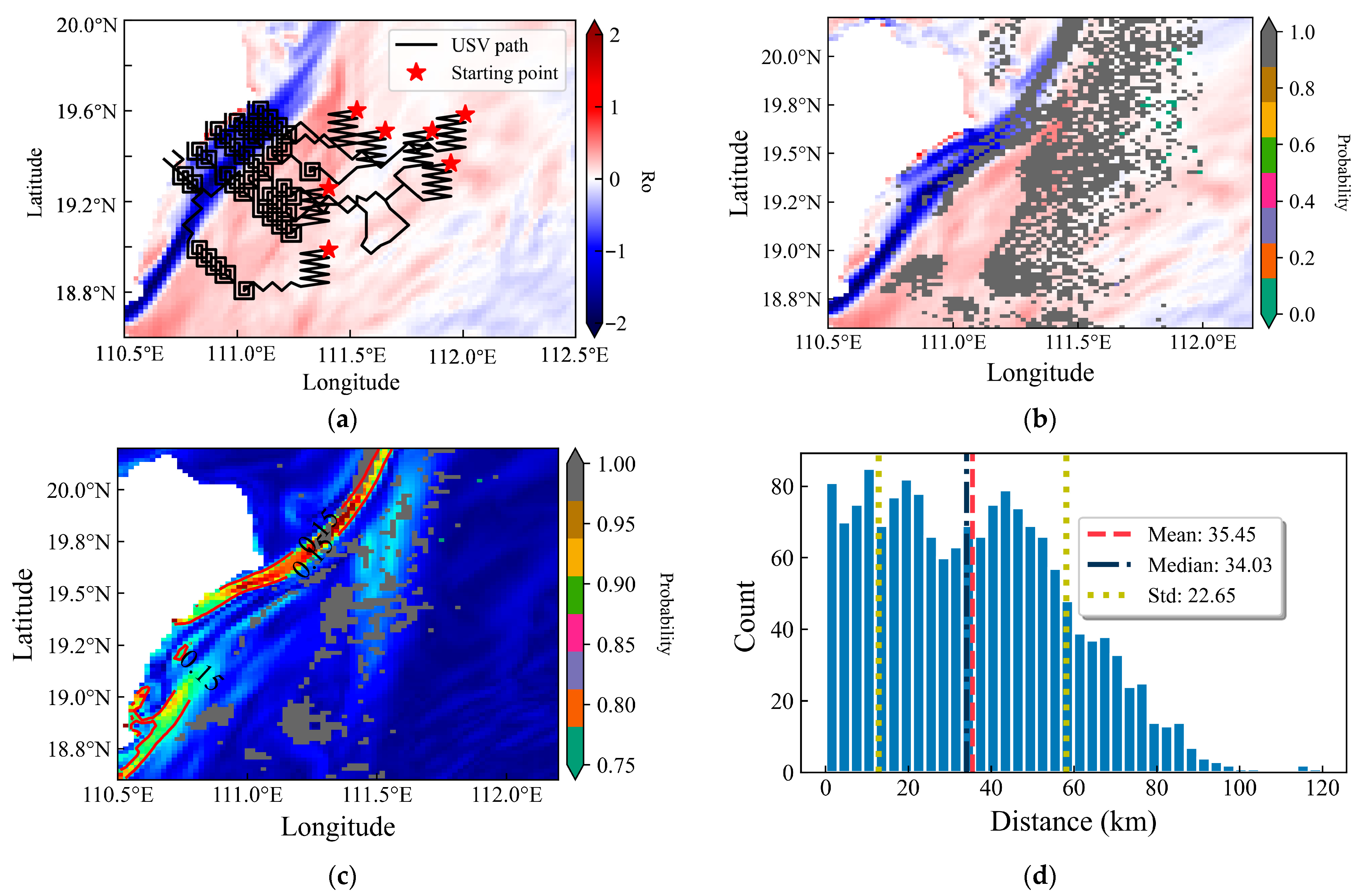
Initialization: A random starting point is selected for the USV, which performs zigzag transect sampling along a predefined orientation (e.g., north to south) at a uniform velocity to collect initial field data including SST, U, and V. The USV is assumed to sample at each grid point it traverses.

(2)

Model Training: Optimal kernel functions and hyper-parameters are configured. All collected data are used to train three separate GPR models—each dedicated to predicting SST, U, and V within the local field—with hyper-parameter optimization performed concurrently for each model.

(3)

Local Field Prediction: The trained GPR models are used to predict SST, U, and V within a local unknown region, defined as a 5 × 5 grid centered on the USV’s current position.

(4)

Adaptive Sampling: The CGI and Ro are calculated across the 5 × 5 grid. The grid point with the maximum CGI value is selected as the next target, and the USV navigates to this location to conduct sampling.

(5)

Intensive Sampling: If the Ro value at any grid point meets the predefined Ro threshold, submesoscale activity is considered probable. If over 60% of the points within the local area satisfy the threshold, the region is classified as actively submesoscale, triggering a spiral-pattern intensive sampling routine. If these conditions are not met, intensive sampling is not activated.

Steps (2) through (5) are repeated iteratively until a predefined number of iterations are completed or the process is manually terminated.

3. Results

Based on the proposed adaptive observation framework, this section presents a comparative analysis of sampling results across different study regions and discusses key factors influencing the performance of the GPR model.

3.1. Optimization of GPR Kernel Functions

The predictive performance of GPR is largely governed by the choice of kernel function, making kernel selection a critical step in model construction. Single kernel functions often exhibit limited flexibility when modeling complex oceanic processes, thus, combining different kernel functions can enhance model capability and lead to improved performance [28,32]. In addition to kernel structure, the suitability of hyper-parameters significantly influences model effectiveness. In this study, the length scale $l$ is initialized as the mean coordinate variance of the training data, and the signal variance ${\sigma }_f^2$ is set to the variance of the target values in the training targets. Hyper-parameters are optimized automatically using the MLM method outlined in Section 2.2. This section focuses on identifying effective composite kernel functions for submesoscale field prediction.

3.1.1. Local Field Prediction Performance

The term “local field” in this study denotes a 5 × 5 grid area centered on the instantaneous position of the USV. During the initial navigation phase, observational data collected along the USV’s path are used to train the GPR models, enabling the generation of predictive information for each local field. The accuracy of these predictions is highly dependent on the choice of kernel function and its associated hyper-parameters, which in turn govern the rationality of subsequent target point selection.

To evaluate the predictive accuracy of GPR under different kernel combinations in localized settings, a dynamically active subregion within area A1—characterized by the most significant SST variations—was selected. A fixed observation path was deliberately designed to traverse zones of high SST gradient (Figure 6), allowing systematic assessment of model performance as the USV transits through regions of significant thermal variability.

Upon reaching a waypoint, the USV collects data instantaneously. These data are combined with all previously acquired measurements to retrain the GPR models. The updated models are then used to predict the SST, U, and V within the local field.

Throughout the observation process, the computational time required for training the GPR models increased progressively with accumulating data volume. By the conclusion of the observation, the final model training time reached approximately 10 s (Figure 7), presenting a potential challenge for real-time operational applications. It should be noted, however, that the fixed lawnmower-path sampling pattern utilized a significantly higher point density compared to the adaptive sampling strategy described in Section 3.2. Consequently, the computational burden associated with the fixed-path approach was substantially greater than that of the adaptive method.

To investigate whether there exist statistically significant differences in the performance of different kernel function combinations, we systematically evaluated the performance differences among various kernel function configurations by conducting paired t-tests with Bonferroni correction on the root mean square error (RMSE) values of SST predictions using GPR from

Table 1. RMSE of SST predictions using GPR with different kernel functions.

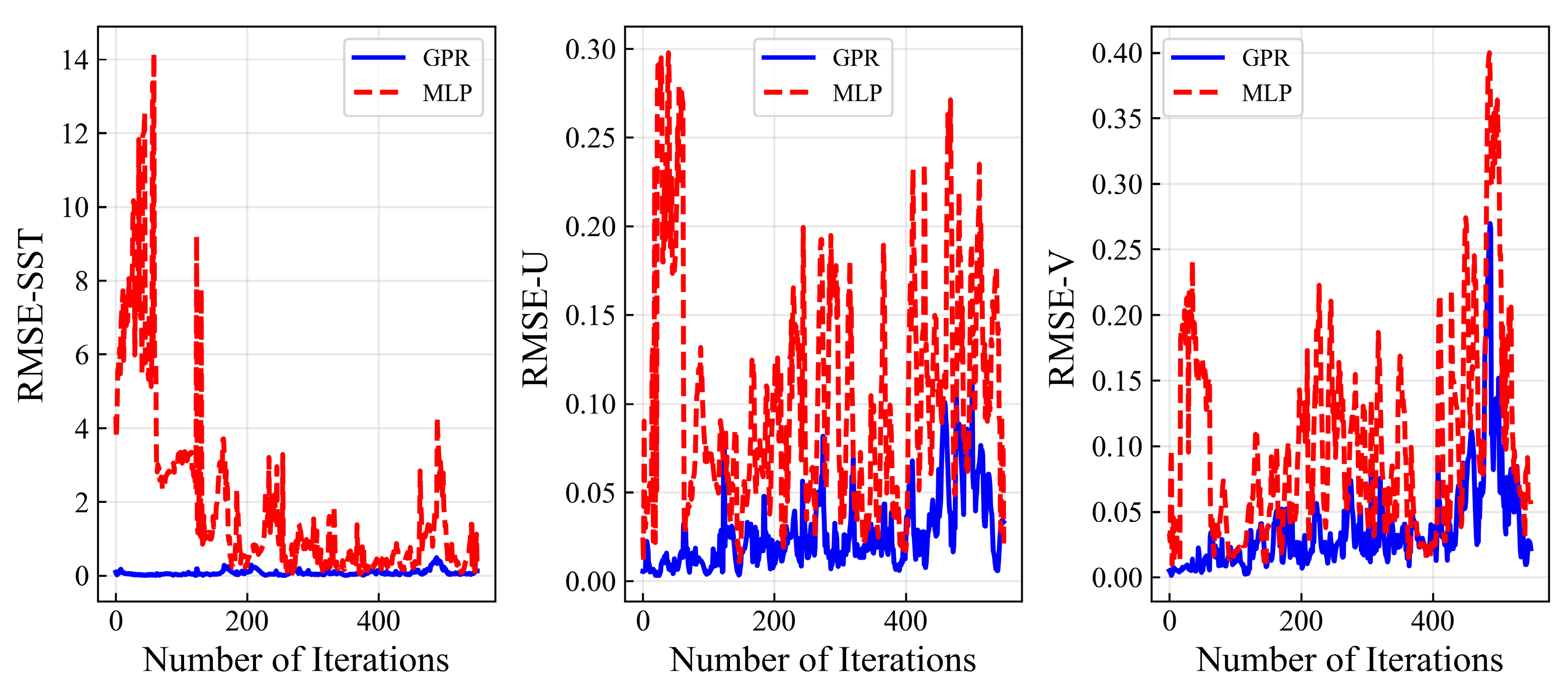
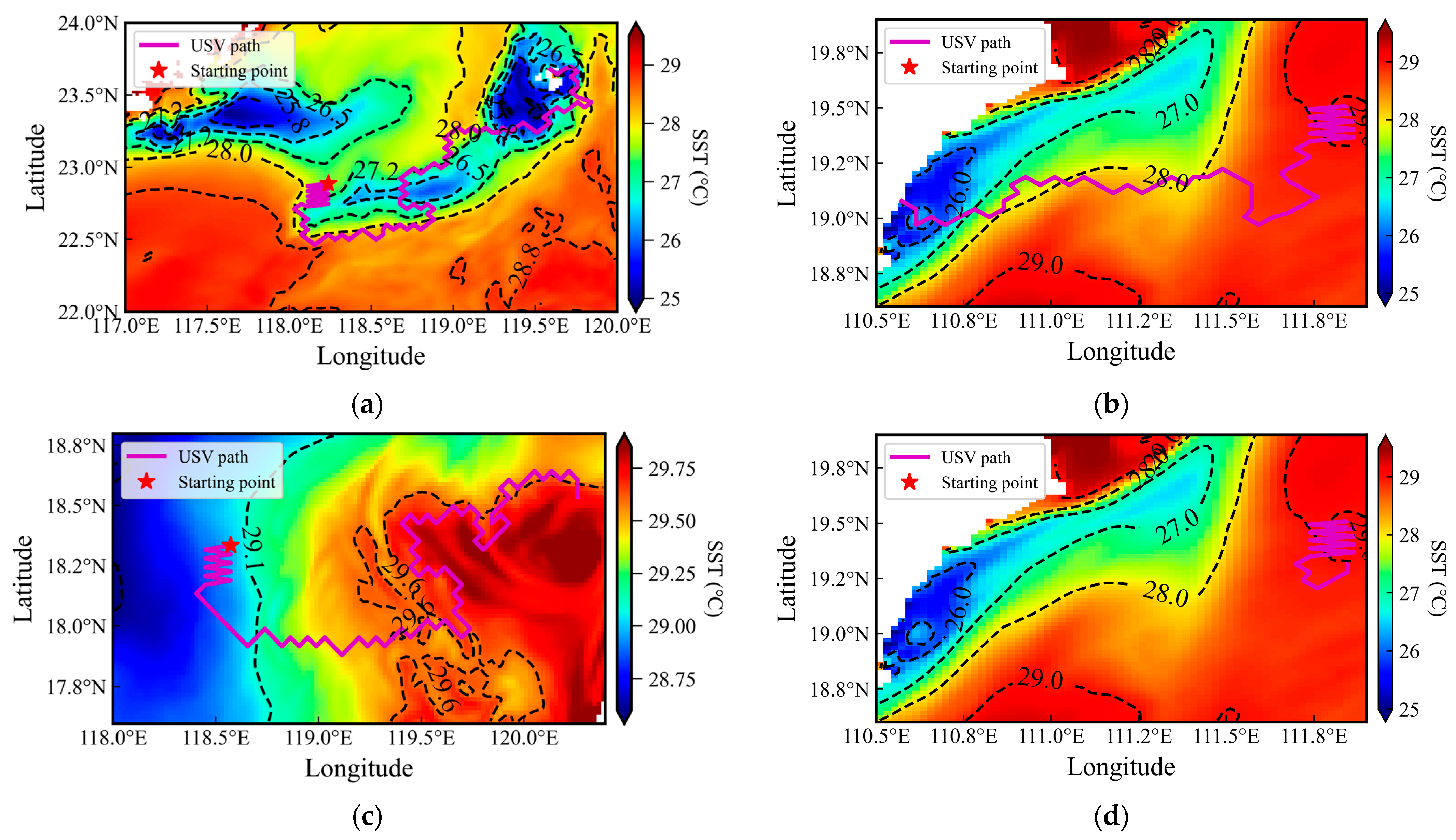
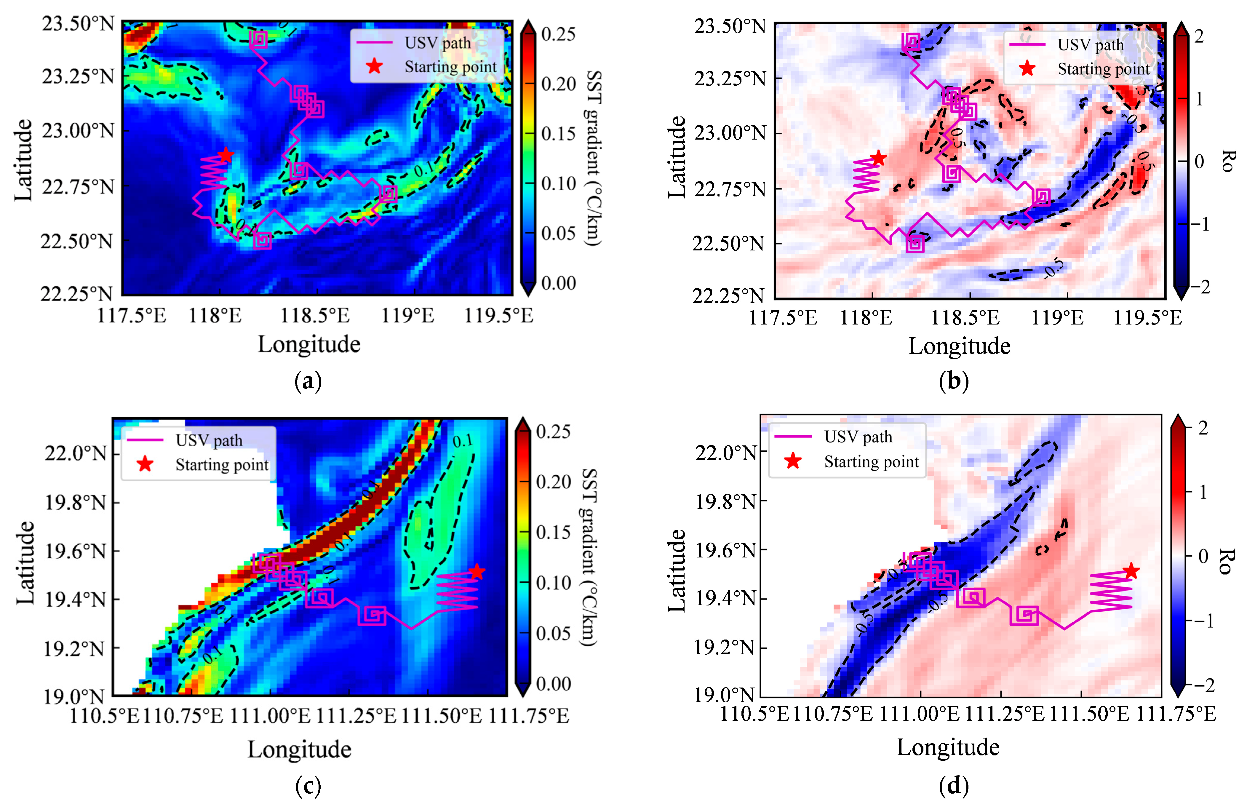
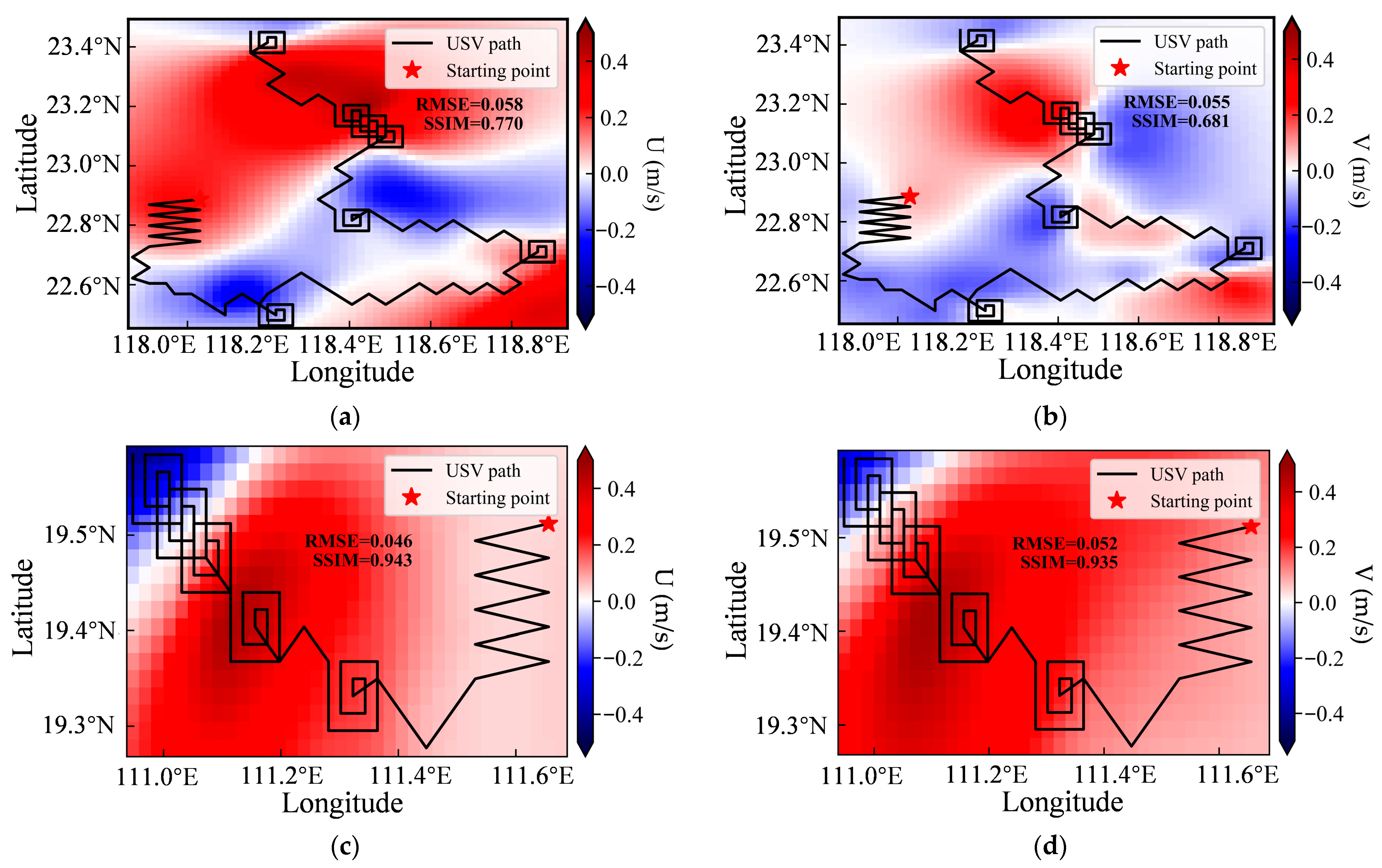
	Mean RMSE
Variables and 95% Confidence Interval
Kernel Function	SST	95%CI	U	95%CI	V	95%CI
Linear	3.701	[3.545, 3.858]	0.123	[0.117, 0.130]	0.120	[0.110, 0.129]
RBF + Matérn32	0.078	[0.071, 0.083]	0.026	[0.025, 0.028]	0.036	[0.033, 0.039]
RBF + Exponential	0.181	[0.176, 0.202]	0.029	[0.027, 0.031]	0.037	[0.034, 0.040]
RBF + Linear	0.385	[0.352, 0.377]	0.340	[0.032, 0.036]	0.042	[0.038, 0.045]
Matérn32 + Exponential	0.080	[0.074, 0.086]	0.026	[0.024, 0.028]	0.036	[0.033, 0.039]
Matérn32 + Linear	0.080	[0.076, 0.089]	0.026	[0.025, 0.028]	0.036	[0.033, 0.039]
Exponential + Linear	0.102	[0.095, 0.108]	0.032	[0.031, 0.034]	0.040	[0.037, 0.043]

. Based on 550 iterations along the fixed path in Figure 6a, sufficient RMSE datasets (550 sets each) were obtained for SST, U, and V variables. The significance analysis reveals that, for SST predictions, statistically significant differences exist between all pairwise kernel function combinations, indicating that kernel selection substantially influences SST prediction performance (Figure 8). In contrast, for U and V predictions, no significant differences were observed between ME and RM, ML and RM, ML and ME, and EL and RL kernel pairs, demonstrating comparable effectiveness of these kernel combinations in predicting ocean current components. This comparative result suggests that SST predictions are more sensitive to kernel selection, while U and V predictions exhibit better adaptability to specific kernel combinations.

A comparative analysis of the averaged RMSE and mean error (MAE) throughout the prediction process showed that the Matérn32 + RBF kernel combination yielded the lowest RMSE and MAE values for SST predictions. For U and V, the three kernel combinations performed similarly (Table 1). The Matérn32 + Linear kernel was selected for velocity predictions due to its ability to generate smoother USV paths. This reduces zigzag movements and frequent turns during observation (even without showing figures), which saves energy by reducing constant turning. The smoothing is relative—the path remains flexible enough to cross areas with significant gradients, and it does not prevent the USV from exploring sharp features in the data. Under these optimal kernel combinations, the mean RMSE and MAE were calculated as (0.078, 0.059) for SST, (0.026, 0.020) for U, and (0.036, 0.028) for V, respectively (Figure 9).

3.1.2. Global Field Reconstruction Accuracy

Global field reconstruction refers to the prediction of the entire environmental field using trained GPR models after all the data has been collected. The field is defined by the range of the USV path. To determine the optimal combination of kernel functions for predicting the global field and assess the stability of their performance across varying sampling densities, we employed a stratified uniform sampling method (Figure 10a). In this approach, we randomly selected 100, 200, 500, and 1000 sampling points for our experiments.

Randomly selected sampling points were used to train the GPR models, which were then applied to predict SST, U, and V across the global field. A1 was chosen as the experimental region due to its significant SST and ocean current variations, as well as a higher concentration of submesoscale features. These characteristics pose a significant challenge for GPR models, thus offering the most rigorous test for evaluating their prediction performance.

Figure 10b–d present the differences between the actual and predicted fields based on 1000 sampling points. The prediction error for SST is within ±0.5 °C, while the errors for the U and V velocity components are within ±0.2m/s. The optimal kernel function combination was determined by comparing the RMSE of GPR predictions for SST, U, and V under different kernel functions. To minimize random variability, each sampling configuration was repeated 50 times, and the RMSE values were averaged.

As shown in

Table 2. RMSE of SST predictions using GPR with different kernel functions (averaged over 50 repetitions).

	RMSE (50-Run Average)								Mean
	Number of Sampling Points and 95% Confidence Interval
Kernel Function	100	95%CI	200	95%CI	500	95%CI	1000	95%CI
Linear	9.875	[9.875, 9.875]	9.844	[9.844, 9.844]	9.849	[9.849, 9.849]	9.823	[9.823, 9.823]	9.848
RBF + Matérn32	0.373	[0.371, 0.374]	0.281	[0.279, 0.284]	0.170	[0.170, 0.170]	0.102	[0.102, 0.102]	0.232
RBF + Exponential	0.380	[0.380, 0.380]	0.293	[0.292, 0.293]	0.181	[0.181, 0.181]	0.110	[0.110, 0.110]	0.241
RBF + Linear	0.566	[0.566, 0.566]	0.544	[0.544, 0.544]	0.224	[0.224, 0.224]	0.172	[0.172, 0.172]	0.377
Matérn32 + Exponential	0.376	[0.376, 0.376]	0.294	[0.294, 0.294]	0.172	[0.172, 0.172]	0.103	[0.103, 0.103]	0.236
Matérn32 + Linear	0.394	[0.394, 0.394]	0.326	[0.326, 0.326]	0.174	[0.174, 0.174]	0.104	[0.104, 0.104]	0.250
Exponential + Linear	0.376	[0.376, 0.376]	0.294	[0.294, 0.294]	0.181	[0.181, 0.181]	0.110	[0.110, 0.110]	0.240

,

Table 3. RMSE of U predictions using GPR with different kernel functions (averaged over 50 repetitions).

	RMSE (50-Run Average)								Mean
	Number of Sampling Points and Confidence Interval
Kernel Function	100	95%CI	200	95%CI	500	95%CI	1000	95%CI
Linear	0.151	[0.151, 0.151]	0.147	[0.147, 0.147]	0.147	[0.147, 0.147]	0.147	[0.147, 0.147]	0.148
RBF + Matérn32	0.085	[0.085, 0.085]	0.075	[0.075, 0.075]	0.040	[0.040, 0.040]	0.034	[0.034, 0.034]	0.059
RBF + Exponential	0.086	[0.086, 0.086]	0.078	[0.070, 0.070]	0.042	[0.042, 0.042]	0.038	[0.038, 0.038]	0.061
RBF + Linear	0.099	[0.099, 0.099]	0.077	[0.077, 0.072]	0.074	[0.074, 0.074]	0.036	[0.036, 0.036]	0.072
Matérn32 + Exponential	0.086	[0.086, 0.086]	0.070	[0.070, 0.070]	0.042	[0.042, 0.042]	0.034	[0.034, 0.034]	0.058
Matérn32 + Linear	0.085	[0.085, 0.085]	0.070	[0.070, 0.070]	0.041	[0.041, 0.041]	0.034	[0.034, 0.034]	0.058
Exponential + Linear	0.086	[0.086, 0.086]	0.070	[0.070, 0.070]	0.042	[0.042, 0.042]	0.038	[0.038, 0.038]	0.059

and

Table 4. RMSE of V predictions using GPR with different kernel functions (averaged over 50 repetitions).

	RMSE (50-Run Average)								Mean
	Number of Sampling Points and Confidence Interval
Kernel Function	100	95%CI	200	95%CI	500	95%CI	1000	95%CI
Linear	0.149	[0.149, 0.149]	0.142	[0.142, 0.142]	0.142	[0.142, 0.142]	0.142	[0.142, 0.142]	0.144
RBF + Matérn32	0.101	[0.101, 0.101]	0.101	[0.101, 0.101]	0.052	[0.052, 0.052]	0.037	[0.037, 0.037]	0.073
RBF + Exponential	0.099	[0.099, 0.099]	0.093	[0.093, 0.093]	0.055	[0.055, 0.055]	0.040	[0.040, 0.040]	0.072
RBF + Linear	0.104	[0.104, 0.104]	0.105	[0.105, 0.105]	0.090	[0.090, 0.090]	0.040	[0.040, 0.040]	0.085
Matérn32 + Exponential	0.099	[0.099, 0.099]	0.093	[0.093, 0.093]	0.055	[0.055, 0.055]	0.040	[0.040, 0.040]	0.072
Matérn32 + Linear	0.101	[0.101, 0.101]	0.101	[0.101, 0.101]	0.052	[0.052, 0.052]	0.037	[0.037, 0.037]	0.073
Exponential + Linear	0.099	[0.099, 0.099]	0.093	[0.093, 0.093]	0.055	[0.055, 0.055]	0.040	[0.040, 0.040]	0.072

, using a single linear kernel function results in the worst reconstruction performance, as indicated by the peak RMSE values observed across all global fields (SST, U, and V). This suggests that the distributions of SST, U, and V in the study area do not follow simple linear spatial trends but instead demonstrate regionally complex non-linear variations. In contrast, the RMSE values corresponding to the combined kernel functions are significantly lower, and as the number of sampling points increases, the RMSE steadily decreases.

Similarly, to investigate whether there are statistically significant differences in the performance of different kernel function combinations, we performed paired t-tests with Bonferroni correction on the kernel combinations in Table 2, Table 3 and Table 4. We randomly selected 100, 200, 500, and 1000 points as training data, with each set of points repeated 50 times. No random seed was set, ensuring different random points in each repetition, but the same points were used across all kernel combinations to enhance comparability. For the global predictions of SST, U, and V, statistically significant differences were found between all pairwise kernel combinations, even though the mean RMSE values of some pairs appeared identical. The significance heatmap was identical to Figure 8a and thus is not shown.

Based on the comprehensive prediction performance of GPR models in the global field, the kernel combinations RBF + Matérn32, Matérn32 + Linear, and Matérn32 + Exponential are identified as the optimal kernel functions for SST, U, and V predictions, respectively. As shown in Table 2, the RBF + Matérn32 combination achieves the smallest mean RMSE for global SST prediction, making it unambiguously the optimal choice. For global U prediction (Table 3), both Matérn32 + Exponential and Matérn32 + Linear yield the same minimum mean RMSE; however, the latter demonstrates better individual performance, thus being selected as the optimal combination. Regarding global V prediction (Table 4), RBF + Exponential, Matérn32 + Exponential, and Exponential + Linear exhibit identical mean RMSE values (maintained to three decimal places), indicating comparable average predictive accuracy. However, the statistically significant differences detected by paired t-tests between these kernel pairs likely stem from differences in performance stability (variance) across the 50 independent runs. This suggests that, while these kernels deliver practically equivalent mean performance, they may differ in their prediction consistency. In light of the identical mean RMSE values, we selected the combination with the smallest variance, namely RBF + Exponential, to ensure more stable prediction performance.

From a physical standpoint, oceanic fields such as SST and currents (U, V) exhibit complex, multiscale spatial structures. Our kernel selection directly reflects this reality. The RBF kernel generates very smooth and stationary functions, making it ideal for capturing the large-scale, globally varying background, dominated by low-frequency, smooth variations. In contrast, the Matérn32 kernel is designed to model rougher and more variable processes. It produces functions that exhibit stronger variability over short distances compared to the RBF kernel, enabling it to effectively capture localized, complex features characteristic of small-scale ocean dynamics, such as the sharp frontal in both SST and velocity fields.

The distinct second kernels for the velocity components further refine this physical interpretation. The use of the Exponential kernel for U aligns with the presence of even rougher, more discontinuous structures in the zonal current. Meanwhile, the application of the RBF kernel for V suggests that its large-scale organizational patterns are notably smoother, sharing a key characteristic with the SST field.

The additive combination of these kernels allows our model to represent the sea surface state as a superposition of a smooth background flow and rough, localized anomalies, a decomposition that is well-grounded in ocean dynamics and contributes to the model’s robust predictive performance.

3.1.3. GPR vs. MLP

To compare the prediction performance of GPR, we developed an MLP model with a dual-hidden-layer architecture. The network structure consists of an input layer with two neurons for latitude and longitude coordinates and an output layer with three neurons corresponding to SST, U, and V components. The hidden layer configuration was determined using the empirical formula H = n/[5 × (I + O)] [33], where n represents the training sample size, while I and O denote the number of input and output nodes, respectively. This yielded 22 neurons in the first hidden layer and 11 in the second. The model was trained using the Adam optimizer with ReLU activation functions and L2 regularization to prevent overfitting. We implemented an adaptive learning rate strategy with a maximum of 2000 iterations and employed early stopping to halt training when validation loss ceased to improve, thereby balancing model performance with computational efficiency.

All experiments were conducted in area A1, where the USV followed the fixed path illustrated in Figure 6a, adhering to the observation procedures outlined in Section 3.1.1. The GPR was configured with its optimal kernel function for local field prediction. Under identical training data conditions, we performed two comparative experimental sets, completing a total of 550 training and prediction cycles.

The results clearly demonstrate the performance advantage of GPR over MLP. As shown in Figure 11, the MLP predictions exhibit notable limitations across all three target variables (SST, U, and V). The RMSE of MLP predictions are substantially higher than those achieved by GPR, with particularly pronounced discrepancies in SST predictions. Furthermore, MLP predictions show significantly larger fluctuations throughout the 550 experimental trials, indicating unstable performance. This considerable variance in prediction errors suggests the model’s difficulty in consistently capturing the underlying physical relationships, likely due to its sensitivity to initial conditions and limited generalization capability on the available dataset. In contrast, GPR maintains consistently lower error levels with minimal fluctuations, demonstrating superior robustness in modeling complex oceanographic processes.

These findings align with established research in small-sample learning scenarios. Previous studies have shown that model selection must carefully consider specific prediction task characteristics. For instance, in predicting cold spray coating manufacturing parameters, both GPR and neural networks have demonstrated optimal performance for different parameter prediction tasks, highlighting the importance of task-specific model selection [34]. Similarly, in groundwater quality prediction with scarce monitoring data, an improved GPR method based on virtual sample generation technology significantly outperformed traditional neural network models in predicting strontium ion concentration. Notably, this approach revealed that model performance peaked when generated virtual samples reached 6–7 times the original data volume, beyond which prediction accuracy decreased—providing valuable guidance for sample augmentation strategies in small-sample learning [35].

Based on these experimental results and supporting literature, we selected GPR for subsequent adaptive sampling tasks. The choice is justified by several key advantages: GPR features a simple structure, computational efficiency, and strong adaptability, making it particularly suitable for processing small to medium-sized datasets. Crucially, GPR not only provides predictive values but also delivers corresponding uncertainty estimates, enabling accurate identification of high-uncertainty regions for optimized sampling paths. The mathematical architecture based on kernel functions offers good interpretability, and our experimental results confirm its significantly better predictive stability compared to alternative methods. While neural networks typically require large-scale training data and involve complex structures with numerous hyperparameters demanding meticulous design and frequent optimization, GPR achieves superior performance with limited data—particularly valuable in adaptive observation scenarios where training time and real-time requirements present critical constraints.

3.2. Performance of the Adaptive Sampling Strategy

The predictive fields generated by GPR models provide the foundation for adaptive sampling. Using this prediction, a frontal search is first conducted to identify candidate regions for submesoscale exploration. When the local Ro satisfies a predefined threshold, intensive sampling is automatically triggered. Following the observation campaign, the complete dataset is used to reconstruct the global environmental field.

3.2.1. Gradient-Based Frontal Search

Regions exhibiting submesoscale processes are typically characterized by strong SST gradients, which result from intense vertical currents that transport cooler subsurface waters to the surface, forming distinct SST fronts as observed in areas A1 and A2. However, in area A3, submesoscale activity deviates from this pattern, showing elevated surface temperatures likely influenced by background oceanic currents [36]. To accommodate such variability, our approach selects the next target point based on the maximum CGI value, ensuring that the observational path captures regions of significant gradient change irrespective of gradient polarity. A key advantage of this strategy is its ability to detect a broader range of submesoscale, including cases with weaker vertical currents where SST gradient may be less pronounced, as illustrated in Figure 10c.

For each of the three study regions, a random starting point was selected. Under optimal model configurations, the USV followed a predefined zigzag path from north to south, systematically collecting 20 samples of SST, U, and V. These spatial datasets were used to train GPR models online, with optimal hyper-parameters optimized iteratively using the MLM method. The trained models were then applied to predict local fields over a 5 × 5 grid.

After obtaining the local field predictions from the GPR models, the maximum CGI value was automatically identified to dynamically select the next target observation point. This decision-making mechanism directs the USV toward regions with strong gradients or, in their absence, toward areas of high predictive uncertainty. Data collected in these regions subsequently enhance model performance by reducing uncertainty in key areas. Guided by this criterion, the USV autonomously adjusts its path toward the selected target. The entire process—including data collection, model retraining, field prediction, and CGI-based path planning—iterates until predefined termination conditions, such as a maximum iteration count, are met.

As shown in Figure 12a–c, the USV observation paths vary in length and duration across the three regions. Despite these differences, the CGI-based strategy consistently guides the USV toward zones of significant SST variation. All paths cross multiple isotherms, confirming alignment with the direction of the strong SST gradient. Although the limited number of iterations restricted more comprehensive spatial coverage, the paths successfully achieved the objective of gradient-oriented search. Nevertheless, the current paths demonstrate that the target of gradient search has been effectively realized. Furthermore, these paths traverse areas exhibiting pronounced strain rate fluctuations, suggesting the likely presence of submesoscale processes and providing a robust foundation for their targeted exploration.

Figure 12d illustrates a failure case originating from the same starting point and model settings as Figure 10b, differing only in the waypoint selection strategy. In this scenario, the next target point was selected by maximizing the SST gradient magnitude. This approach led to an operational deadlock: following the initial zigzag transit, the USV entered a sustained oscillatory state. The underlying cause was the presence of an SST extremum within the local field. Each time the USV arrived at a target location, the SST gradient computation designated the previous waypoint as the subsequent target, resulting in a cyclic to-and-fro motion that halted further gradient search progress.

These results demonstrate that the CGI strategy substantially improves the robustness of USV guidance by minimizing the risk of entrapment at local gradient extrema. This enhancement arises from the integration of multiple variables, which diminishes sensitivity to anomalies in any single parameter and promotes more stable path planning. It is noteworthy that, within the study area, the SST gradient remained the dominant influence, resulting in a clear alignment of the USV’s path with thermally dynamic zones marked by pronounced SST variations.

3.2.2. Triggered Intensive Sampling of Submesoscale Features

During the gradient search phase, the USV has autonomously identified regions characterized by strong SST gradients. Building on this capability, a Ro threshold is introduced as an additional diagnostic criterion to confirm the presence of submesoscale activity around these high-gradient areas.

As described in Section 2.4.3, submesoscale activity is identified when the Ro value falls within the range of 0.5 to 2. During adaptive gradient searches, the Ro is computed for each local field. If more than 60% of the grid points within a field meet this threshold, the region is classified as exhibiting active submesoscale phenomena, triggering targeted high-resolution data sampling.

To acquire high-resolution submesoscale data, a full-coverage spiral sampling pattern (Figure 13) is implemented in local fields identified as active submesoscale. Initiated from the grid center, this strategy: (1). ensures comprehensive spatial data collection, facilitating detailed offline analysis; and (2). enhances observational efficiency by following a non-overlapping spiral path, thereby eliminating redundant coverage during intensive sampling operations.

Using randomly selected starting points, the GPR model—equipped with optimized kernel functions and hyper-parameters and integrated with the CGI strategy and Ro threshold—performed adaptive exploration and intensive sampling of submesoscale. The spiral sampling path was triggered in local areas where the Ro threshold was satisfied, successfully capturing high-resolution data within submesoscale structures (Figure 14).

In Figure 14, the background in the left column represents the SST gradient, while the right column shows the Ro distribution. SST gradients are not uniformly distributed, and their magnitudes vary considerably across regions. Specifically, regions A1 and A2 exhibit more complex SST variations and spatial patterns, whereas A3 shows the weakest gradient signals. In A1 and A2, the USV’s path clearly traverses zones of strong SST gradient isotherms, confirming successful gradient-guided navigation and the effective execution of intensive sampling in dynamically active areas. Although SST gradients are weaker in A3, the CGI-based approach still enabled the USV to actively explore the environment and detect submesoscale activity. A total of six, five, and three intensive sampling events were triggered in A1, A2, and A3, respectively. Continued operation would allow for additional sampling, with intensive sampling number naturally increasing in regions richer in submesoscale features. Across all regions, the USV demonstrated autonomous exploration and response capabilities, validating the effectiveness of the proposed adaptive observation strategy for submesoscale oceanic processes.

As mentioned above, intensive observations are primarily triggered by the Ro threshold. However, for submesoscale processes, there is currently no precise numerical definition for Ro, only an order-of-magnitude estimate. This definitional uncertainty leads to a practical issue: the choice of the Ro threshold significantly influences the outcomes of adaptive sampling strategies.

To evaluate the sensitivity of the threshold settings, we conducted two contrasting experiments in region A2: one with a narrower threshold range (0.8–1.5) and another with a broader threshold range (0.2–2.2). The test results clearly demonstrate that the choice of threshold range has a decisive impact on the triggering of intensive observations (Figure 15). Specifically, the narrower threshold (0.8–1.5), due to its more stringent criteria, triggered only two enhanced observation events throughout the study period. In contrast, the broader threshold (0.2–2.2), by encompassing a wider range of dynamical processes, triggered as many as seven events. This finding directly confirms that the frequency of intensive observations is positively correlated with the width of the Ro threshold.

It should be noted that the intensive sampling process was not perfectly precise, particularly in regions such as A2. In some cases, intensive sampling was triggered in locations lacking clear submesoscale signatures—a phenomenon termed “false intensive sampling”. This is likely attributable to inaccuracies in the GPR-predicted velocity components (U, V), which led to discrepancies between the computed and actual Ro values. Nonetheless, these errors had a minimal impact on the overall adaptive sampling performance, as the USV consistently converged toward regions with active submesoscale features.

The occurrence of false intensive sampling arises from differences in Ro calculation methods. As shown in Figure 16, the local Ro values derived from GPR-predicted velocity fields are generally higher than those obtained from the true global Ro field. This systematic overestimation helps explain the erroneous triggering of intensive sampling in areas that do not satisfy the Ro threshold. The scale-dependent behavior of Ro and its underlying mechanisms require further investigation.

3.2.3. Post-Mission Environmental Field Reconstruction

After completing the observation process, the data collected along the USV’s path were used to train GPR models and reconstruct the environmental field across the sampled region. As outlined in Section 3.1.2, the global SST field was predicted using the Matérn32 + RBF kernel combination in the GPR model. The resulting reconstruction provides an initial characterization of the environmental structure without relying on prior knowledge, thereby facilitating the design of subsequent targeted observation strategies. The spatial extent of the reconstructed field was defined to fully encompass the USV path, with its four vertices determined by the minimum and maximum coordinates recorded along the path.

As shown in Figure 17, the left column displays the predicted SST field, while the right column presents the corresponding true SST fields. The RMSE was calculated by comparing these paired fields. In addition to RMSE, the structural similarity index measure (SSIM) was employed to evaluate the perceptual similarity between the predicted and actual SST images, offering a more comprehensive assessment of the GPR model’s reconstruction accuracy.

$$SSIM(1,2)={\displaystyle \frac{(2{\mu }_1{\mu }_2+C_1)(2{\sigma }_{12}+C_2)}{({{\mu }_1}^2+{{\mu }_2}^2+C_1)({{\sigma }_1}^2+{{\sigma }_2}^2+C_2)}}$$

Here, 1 and 2 represent the two images that need to be compared. $C_1$, $C_2$ are default constants, ${\mu }_1$, ${\mu }_2$ are the means of the two images, respectively, ${{\sigma }_1}^2$, ${{\sigma }_2}^2$ are the standard deviations of the two images, and ${\sigma }_{12}$ is the covariance of the two images.

This result demonstrates that the predictive skill of the GPR model is co-influenced by the spatial scale and the inherent complexity of the reconstruction domains. The spatial extent of the three reconstruction domains follows the order A1 > A3 > A2. Accordingly, the RMSE improves sequentially from 0.347 in the largest and most complex domain (A1) to 0.258 in A2 and achieves the best value of 0.066 in the smallest and dynamically simplest domain (A3). In contrast, the SSIM trend does not perfectly mirror the RMSE; it is highest in A3, followed by A1, and is lowest in A2.

The notably higher RMSE in A2 compared to the similarly sized A3 underscores the dominant role of regional complexity, as A2 exhibits more intricate thermal patterns. Furthermore, the fact that the larger and more complex domain A1 achieves a higher SSIM than A2 suggests that the spatial distribution of sampling points in A1 provides a more effective basis for the GPR to reconstruct the underlying environmental structures.

Overall, despite small-scale discrepancies exacerbated by spatial heterogeneity and limited data, the reconstructed fields across all three domains successfully capture the main spatial structures of the true SST fields. This confirms the model’s practical utility in representing SST features across diverse scales and dynamic regimes, with accuracy poised for further improvement through enhanced observational data and optimized sampling strategies.

As shown in Figure 18, the left column presents the predicted U field, and the right column shows the predicted V field. The USV observation paths and the spatial extent of the reconstructed environmental field are consistent with those shown in Figure 17. In accordance with Section 3.1.2, the U field was predicted using the Matérn32 + Exponential kernel function, whereas the V field was reconstructed with the RBF + Matérn32 kernel.

The RMSE of the GPR reconstruction for both U and V fields follows the same trend as that for SST, decreasing progressively from region A1 to A3. However, the trend in SSIM reveals a notable difference. The SSIM is highest in region A2, followed by A3, and is lowest in region A1. This pattern is likely attributable to the high complexity of the flow field in A1, which challenges the model’s ability to reconstruct fine-scale structures, thereby reducing the SSIM. Conversely, the more concentrated and well-defined flow patterns in A2 facilitate a more accurate reconstruction of the field’s spatial features, resulting in the highest SSIM. Despite these variations, the SSIM values in A2 and A3 both exceed 0.9, indicating a high degree of similarity between the predicted and actual fields, and the GPR model demonstrates consistently strong predictive performance across all three regions.

This high-fidelity reconstruction of velocity fields is critical for the subsequent dynamical analysis, as Ro is derived from these velocity components. Only when both velocity predictions are sufficiently accurate can the resulting Ro values be considered reliable, thereby enabling the USV to correctly identify submesoscale features and conduct effective, targeted intensive sampling.

3.3. Analysis of Initial Deployment Locations

SST and current velocity typically exhibit significant spatiotemporal variability across oceanic regions, with their magnitudes and spatial structures strongly dependent on location. Consequently, adaptive sampling strategies initiated from different starting points yield distinct initial observational datasets. When used as input for GPR models, these datasets lead to divergent predictions for optimal subsequent sampling locations. As a result, the resulting sampling paths vary considerably—particularly in terms of path length and search efficiency—depending on the initial deployment position.

Although the examples in Figure 19a successfully capture submesoscale features, this outcome is not assured under random starting-point selection. Owing to the inherent complexity of marine environments, both lawnmower-pattern and adaptive surveys exhibit high sensitivity to the choice of initial location. Thus, the strategic selection of starting points can substantially improve the efficiency of submesoscale feature identification while minimizing redundant or unnecessary sampling efforts.

Using adaptive observations in region A2 as an example, we systematically evaluated the capability to identify submesoscale features by sequentially designating each grid point in the target area as an observation-path starting point. For each of thirty repeated trials, successful identification of submesoscale features was recorded as 1 and failures as 0. As shown in Figure 19b, gray markers indicate grid points where the identification probability reached 1 (against a background of Rossby number, Ro), while other colors represent intermediate probabilities. Owing to the spatially discrete distribution of the gray markers, a 2 × 2 spatial smoothing filter was applied, producing Figure 19c—where the background now shows SST gradient magnitude—which more clearly reveals the spatial clustering of effective starting locations. The results from the five repeated trials showed minimal variation, underscoring the robustness of the GPR predictions.

To statistically evaluate the spatial distribution of successful submesoscale detection starting points, we first identified a prominent SST gradient isopleth (0.15 °C/km). The minimum perpendicular distance from each successful starting point (gray dots, Figure 19b) to this isopleth was then calculated. The resulting distance distribution, as summarized in the histogram in Figure 19d, exhibits a mean of 35.45 km, a median of 34.03 km, and a standard deviation of 22.65 km, with a grid resolution of approximately 2 km. Notably, less than 0.24% of the data falls within the outlier region (determined by quantile analysis), indicating strong statistical robustness. This quantitative assessment of the proximity between detection starting points and SST gradient supports the strategic placement of initialization locations, thereby enhancing both the probability of detection and the efficiency of submesoscale feature exploration.

4. Discussion

Submesoscale processes, characterized by rapid spatiotemporal variability, demand highly agile observation systems for effective monitoring. When operational conditions allow, multiplatform configurations employing advanced coordination strategies can significantly enhance the resolution of spatiotemporal sampling requirements. The GPR-based adaptive observation framework proposed in this study is designed to be scalable; it is applicable not only to single platforms but also extendable to coordinated multiplatform systems. Although the current implementation focuses on static environmental fields, the methodology is inherently adaptable and structured for future extension to dynamic field scenarios.

Kernel function selection plays a crucial role in determining the predictive performance of GPR, particularly when modeling complex, non-linear oceanic dynamics. While the composite kernels used in this work exhibit robust performance, there remains potential for improvement, especially in predicting Ro fields. Therefore, the development of more sophisticated kernel architectures with greater physical interpretability represents a key direction for enhancing the accuracy and reliability of GPR-based environmental inference.

The choice of initial deployment locations is critical for the success of submesoscale observation missions. Due to computational limitations associated with dense spatial grids, this study evaluated each starting point through five independent trials. A binary detection indicator (1 for successful detection, 0 for failure) was recorded per trial, and the arithmetic mean across trials was computed to assess performance. Although inter-trial variations were minimal, increasing the number of repetitions will be necessary in future work to ensure statistical robustness and convergence.

This study utilizes a virtual observation platform based on idealized assumptions: motion control is simplified through sequential waypoint navigation, steering constraints are relaxed to permit 360° omnidirectional turning, and constant velocity is maintained throughout missions. These simplifications serve two purposes: first, to reduce system complexity and focus on evaluating the core observation strategies; second, to maintain authenticity, as these assumptions align with capabilities of existing USV technologies.

5. Conclusions and Future Work

This study introduces a GPR-based adaptive observation strategy for enabling a single USV to autonomously navigate regions of high SST variability and identify submesoscale active zones. Key methodological innovations include the optimization of composite kernel functions. Specifically, distinct optimal composite kernel functions were identified for predicting different variables (SST, U, V) at both local and global scales. Furthermore, a novel CGI is introduced for robust path planning, incorporating the gradients of SST and strain rate, as well as the normalized GPR prediction error. This method enhances robustness by reducing sensitivity to noise and avoiding local gradient extrema traps inherent in traditional navigation strategies. Additionally, adaptive intensive sampling is triggered by predefined Ro thresholds, which initiate targeted data collection such as spiral sampling to intensify coverage in high-interest areas.

Simulation results demonstrate that composite kernels significantly outperform single linear kernels, substantially reducing prediction RMSE across all environmental fields. Reconstruction analyses reveal that, while the RMSEs for SST and velocity (U, V) fields share a common trend (highest in A1, lowest in A3), their respective SSIM trends are distinct and do not mirror the RMSE. This demonstrates that the two metrics capture different aspects of performance, a pattern governed by domain scale, physical complexity, and data distribution. Furthermore, deployment within 35.45 km of the 0.15 °C/km isotherm gradient enhances submesoscale detection probability. This optimization offers practical guidance for the design of USV starting points.

Current limitations include computational latency in GPR retraining, which hinders real-time capture of transient submesoscale processes. To address this, future work will integrate sparse online Gaussian processes (SOGPs) [20] and enhanced variants [37,38] to reduce computational load, data storage requirements, and decision-making latency. This will enable scalable, responsive adaptive sampling for dynamic features like frontogenesis and filamentation. Furthermore, future efforts will focus on enhancing the prediction accuracy of GPR through the development of more sophisticated kernel functions, while also refining deployment strategies to mitigate path sensitivity to initial conditions. This dual approach will ensure more efficient and reliable data acquisition in dynamically evolving marine environments.

References

- McWilliams, J.C. Submesoscale currents in the ocean. Proc. R. Soc. A Math. Phys. Eng. Ing Sci. 2016, 472, 20160117. [Google Scholar] [CrossRef]
- Thomas, L.N.; Tandon, A.; Mahadevan, A. Submesoscale Processes and Dynamics; Hecht, M.W., Hasumi, H., Eds.; American Geophysical Union: Washington, DC, USA, 2008; pp. 17–35. [Google Scholar] [CrossRef]
- Zhang, Z.; Zhang, X.; Qiu, B.; Zhao, W.; Zhou, C.; Huang, X.; Tian, J. Submesoscale Currents in the Subtropical Upper Ocean Observed by Long-Term High-Reso lution Mooring Arrays. J. Phys. Oceanogr. 2021, 51, 187–206. [Google Scholar] [CrossRef]
- Capet, X.; McWilliams, J.C.; Molemaker, M.J.; Shchepetkin, A.F. Mesoscale to Submesoscale Transition in the California Current System. Part III: Energy Balance and Flux. J. Phys. Oceanogr. 2008, 38, 2256–2269. [Google Scholar] [CrossRef]
- D’Asaro, E.; Lee, C.; Rainville, L.; Harcourt, R.; Thomas, L. Enhanced Turbulence and Energy Dissipation at Ocean Fronts. Science 2011, 332, 318–322. [Google Scholar] [CrossRef]
- Guo, M.; Xing, X.; Xiu, P.; Dall’oLmo, G.; Chen, W.; Chai, F. Efficient biological carbon export to the mesopelagic ocean induced by submesoscale fronts. Nat. Commun. 2024, 15, 580. [Google Scholar] [CrossRef]
- Zhang, Z.; Miao, M.; Qiu, B.; Tian, J.; Jing, Z.; Chen, G.; Chen, Z.; Zhao, W. Submesoscale Eddies Detected by SWOT and Moored Observations in the Northwestern Pacific. Geophys. Res. Lett. 2024, 51, e2024GL110000. [Google Scholar] [CrossRef]
- Yang, H.; Chen, Z.; Sun, S.; Li, M.; Cai, W.; Wu, L.; Cai, J.; Sun, B.; Ma, K.; Ma, X.; et al. Observations Reveal Intense Air-Sea Exchanges Over Submesoscale Ocean Front. Geophys. Res. Lett. 2024, 51, e2023GL106840. [Google Scholar] [CrossRef]
- Dong, J.; Fox-Kemper, B.; Zhang, H.; Dong, C. The Scale and Activity of Symmetric Instability Estimated from a Global Submesoscale-Permitting Ocean Model. J. Phys. Oceanogr. 2021, 51, 1655–1670. [Google Scholar] [CrossRef]
- Nagano, A.; Ando, K. Saildrone-observed atmospheric boundary layer response to winter mesoscale warm spot along the Kuroshio south of Japan. Prog. Earth Planet. Sci. 2020, 7, 43. [Google Scholar] [CrossRef]
- Tang, H.; Wang, D.; Shu, Y.; Yu, X.; Shang, X.; Qiu, C.; Yu, J.; Chen, J. Vigorous Forced Submesoscale Instability Within an Anticyclonic Eddy During Tropical Cyclone “Haitang” from Glider Array Observations. J. Geophys. Res. Ocean. 2025, 130, e2024JC021396. [Google Scholar] [CrossRef]
- Nagano, A.; Geng, B.; Richards, K.J.; Cronin, M.F.; Taniguchi, K.; Katsumata, M.; Ueki, I. Coupled Atmosphere–Ocean Variations on Timescales of Days Observed in the Western Tropical Pacific Warm Pool During Mid-March 2020. J. Geophys. Res. Ocean. 2022, 127, e2022JC019032. [Google Scholar] [CrossRef]
- Belkin, I.; de Sousa, J.B.; Pinto, J.; Mendes, R.; Lopez-Castejon, F. A new front-tracking algorithm for marine robots. In Proceedings of the 2018 IEEE/OES Autonomous Underwater Vehicle Workshop (AUV), Porto, Portugal, 6–9 November 2018; pp. 1–3. [Google Scholar] [CrossRef]
- Mitarai, S.; McWilliams, J.C. Wave glider observations of surface winds and currents in the core of Typhoon Danas. Geophys Ical Res. Lett. 2016, 43, 11312–11319. [Google Scholar] [CrossRef]
- Woithe, H.C.; Kremer, U. Feature based adaptive energy management of sensors on autonomous underwater vehicles. Ocean Eng. 2015, 97, 21–29. [Google Scholar] [CrossRef]
- Zhang, Y.; Godin, M.A.; Bellingham, J.G.; Ryan, J.P. Using an Autonomous Underwater Vehicle to Track a Coastal Upwelling Front. IEEE J. Ocean. Eng. 2012, 37, 338–347. [Google Scholar] [CrossRef]
- Petillo, S.; Schmidt, H.; Lermusiaux, P.; Yoerger, D.; Balasuriya, A. Autonomous & adaptive oceanographic front tracking on board autonomous underwater vehicles. In Proceedings of the OCEANS 2015, Genova, Italy, 18–21 May 2015; pp. 1–10. [Google Scholar] [CrossRef]
- Rasmussen, C.E.; Williams, C.K.I. Gaussian Processes for Machine Learning; The MIT Press: Cambridge, MA, USA, 2005; ISBN 978-0-262-25683-4. Available online: https://direct.mit.edu/books/oa-monograph/2320/Gaussian-Processes-for-Machine-Learning (accessed on 19 July 2025).
- Ma, K.C.; Ma, Z.; Liu, L.; Sukhatme, G.S. Multi-robot Informative and Adaptive Planning for Persistent Environmental Monitoring. In Proceedings of the Distributed Autonomous Robotic Systems: The 13th International Symposium, London, UK, 7–9 November 2016; pp. 285–298. [Google Scholar] [CrossRef]
- Ma, K.C.; Liu, L.; Heidarsson, H.K.; Sukhatme, G.S. Data-driven learning and planning for environmental sampling. J. Field Robot. 2018, 35, 643–661. [Google Scholar] [CrossRef]
- Fossum, T.O.; Eidsvik, J.; Ellingsen, I.; Alver, M.O.; Fragoso, G.M.; Johnsen, G.; Mendes, R.; Ludvigsen, M.; Rajan, K. Information-driven robotic sampling in the coastal ocean. J. Field Robot. 2018, 35, 1101–1121. [Google Scholar] [CrossRef]
- Wang, S.; Song, Z.; Ma, W.; Shu, Q.; Qiao, F. Mesoscale and submesoscale turbulence in the Northwest Pacific Ocean revealed by numerical simulations. Deep Sea Res. Part II Top. Stud. Oceanogr. 2022, 206, 105221. [Google Scholar] [CrossRef]
- Gallmeier, K.; Prochaska, J.X.; Cornillon, P.; Menemenlis, D.; Kelm, M. An evaluation of the LLC4320 global-ocean simulation based on the submesoscale structure of modeled sea surface temperature fields. Geosci. Model Dev. 2023, 16, 7143–7170. [Google Scholar] [CrossRef]
- Lin, H.; Liu, Z.; Hu, J.; Menemenlis, D.; Huang, Y. Characterizing meso- to submesoscale features in the South China Sea. Prog. Oceanogr. 2020, 188, 102420. [Google Scholar] [CrossRef]
- Zhang, Z.; Liu, Y.; Qiu, B.; Luo, Y.; Cai, W.; Yuan, Q.; Liu, Y.; Zhang, H.; Liu, H.; Miao, M.; et al. Submesoscale inverse energy cascade enhances Southern Ocean eddy heat transport. Nat. Commun. 2023, 14, 1335. [Google Scholar] [CrossRef]
- Stachniss, C.; Plagemann, C.; Lilienthal, A.J.; Burgard, W. Gas Distribution Modeling Using Sparse Gaussian Process Mixture Models. In Robotics: Science and Systems IV; MIT Press: Cambridge, MA, USA, 2008; pp. 310–317. Available online: https://ieeexplore.ieee.org/document/6284842 (accessed on 26 July 2025).
- He, Z.; Liu, G.; Zhao, X.; Yang, J. Temperature Model for FOG Zero-Bias Using Gaussian Process Regression. In Intelligence Computation and Evolutionary Computation; Springer: Berlin/Heidelberg, Germany, 2013; pp. 37–45. [Google Scholar]
- Zhang, Y.; Feng, M.; Zhang, W.; Wang, H.; Wang, P. A Gaussian process regression-based sea surface temperature interpolation algorithm. J. Ocean. Limnol. 2021, 39, 1211–1221. [Google Scholar] [CrossRef]
- Hornik, K.; Stinchcombe, M.; White, H. Multilayer feedforward networks are universal approximators. Neural Netw. 1989, 2, 359–366. [Google Scholar] [CrossRef]
- Zheng, Q.; Xie, L.; Xiong, X.; Hu, X.; Chen, L. Progress in research of submesoscale processes in the South China Sea. Acta Ocean. Sin. 2020, 39, 1–13. [Google Scholar] [CrossRef]
- Zhao, Z.; Liu, B.; Li, X. Internal solitary waves in the China seas observed using satellite remote-sensing techniques: A review and perspectives. Int. J. Remote Sens. 2014, 35, 3926–3946. [Google Scholar] [CrossRef]
- Aravind, H.M.; Özgökmen, T.M.; Allshouse, M.R. Lagrangian analysis of submesoscale flows from sparse data using Gaussian Process Regression for field reconstruction. Ocean Model. 2025, 193, 102458. [Google Scholar] [CrossRef]
- Neural Computing: NeuralWorks Professional II/PLUS and Neural Works Explorer.—Ben-Gurion University of the Negev. Available online: https://primo.bgu.ac.il/discovery/fulldisplay/alma990019863950204361/972BGU_INST:972BGU (accessed on 24 October 2025).
- Citarella, A.A.; Carrino, L.; De Marco, F.; Di Biasi, L.; Perna, A.S.; Viscusi, A.; Tortora, G. AI Data-Driven Optimization of Cold Spray Coating Manufacturing. IEEE Trans. Ind. Inform. 2025, 21, 7848–7858. [Google Scholar] [CrossRef]
- Zhang, J.; Xiao, C.; Yang, W.; Liang, X.; Zhang, L.; Wang, X.; Dai, R. Improving prediction of groundwater quality in situations of limited monitoring data based on virtual sample generation and Gaussian process regression. Water Res. 2024, 267, 122498. [Google Scholar] [CrossRef]
- Katsaros, K.B.; Soloviev, A.V.; Weisberg, R.H.; Luther, M.E. Reduced Horizontal Sea Surface Temperature Gradients Under Conditions of Clear Skies and Weak Winds. Bound. Layer Meteorol 2005, 116, 175–185. [Google Scholar] [CrossRef]
- Melkumyan, A.; Ramos, F. A sparse covariance function for exact Gaussian process inference in large datasets. In Proceedings of the 21st International Joint Conference on Artificial Intelligence, Pasadena, CA, USA, 11–17 July 2009; Morgan Kaufmann Publishers Inc.: San Francisco, CA, USA, 2009; pp. 1936–1942. Available online: https://studylib.net/doc/13900740/a-sparse-covariance-function-for-exact-gaussian-process-i (accessed on 26 July 2025).
- Lawrence, N.; Seeger, M.; Herbrich, R. Fast sparse Gaussian process methods: The informative vector machine. In Proceedings of the 16th International Conference on Neural Information Processing Systems, Bangkok, Thailand, 1–5 December 2009; MIT Press: Cambridge, MA, USA, 2002; pp. 625–632. Available online: https://proceedings.neurips.cc/paper_files/paper/2002/file/d4dd111a4fd973394238aca5c05bebe3-Paper.pdf (accessed on 26 July 2025).