Abstract
We propose a complexity-aware extension of the Course–Speed (CS) model that integrates an AIS-derived Traffic Complexity Index (TCI) based on change in speed (ΔV) and course (Δθ) to quantify maneuvering complexity in nonlinear crossing waters. The framework consists of: (i) data preprocessing and gating to ensure navigationally valid AIS samples; (ii) CS index computation using distribution-aware statistics; (iii) TCI estimation from variability in speed and course along intersecting flows; and (iv) an integrated CS–TCI for interpretable mapping and ranking. Using one year of AIS data from a high-density crossing area near the Korean coast, we show that the integrated index reveals crossing hotspots and small-vessel maneuvering burdens that are not captured by spatial regularity metrics alone. The results remain robust across reasonable parameter ranges (e.g., speed filter and σ-based weighting), and they align with operational observations in vessel traffic services (VTS). The proposed CS–TCI offers actionable decision support for port and coastal operations by jointly reflecting traffic smoothness and complexity; it can complement collision-risk screening and efficiency-oriented planning (e.g., energy and emission considerations). The approach is readily transferable to other crossing waterways and can be integrated with real-time monitoring to prioritize control actions in complex marine traffic environments.
1. Introduction
1.1. Background and Motivation
The expansion of international logistics and the advancement in smart and autonomous shipping technologies have driven a steady increase in maritime traffic volumes worldwide. The maritime sector is also a major source of greenhouse gas (GHG) emissions, contributing nearly 3% of global anthropogenic CO2 emissions, with projections indicating continued growth under a business-as-usual scenario [1]. This growth, while a catalyst for economic development, presents critical challenges related to navigational safety, congestion, and environmental risks. A single maritime accident can lead to severe ecological damage and significant economic loss, undermining the long-term sustainability of the entire shipping industry.
Therefore, developing robust evaluation models capable of analyzing traffic flow regularity and complexity is not merely an operational necessity but a fundamental requirement for building a safe, resilient, and sustainable marine transportation network. Traditional human-based vessel traffic service (VTS) systems exhibit limited scalability and objectivity, necessitating data-driven methodologies for traffic pattern analysis and risk prediction.
1.2. Prior Research and Limitations
Previously, the authors introduced the course–speed (CS) model [2], which enables the quantitative assessment of maritime traffic flow by measuring deviations in course over ground (COG) and speed over ground (SOG) from a standard plan. While this model is effective for evaluating spatiality and continuity in linear fairways, it is based on the assumption of stable, unidirectional traffic patterns. However, such assumptions are inadequate for nonlinear intersectional sea areas, where traffic flows are characterized by multi-directional crossings, complex maneuvering, and increased navigational interactions.
Many recent complexity-aware studies lack a clear link to operational or environmental outcomes, which limits their contribution to sustainability goals. Our proposed model addresses this gap by directly quantifying dynamic maneuvering, a key factor in preventing accidents and enhancing the overall sustainability of maritime operations.
Recent advances in intelligent transportation systems (ITS) and networked control theory have introduced data-driven strategies for analyzing and managing traffic complexity in large-scale, nonlinear environments [3,4]. These studies demonstrate how adaptive learning and coordination frameworks can enhance situational awareness and real-time decision-making in congested traffic networks. Inspired by these developments, the present research extends such complexity-aware principles to the maritime domain, where vessel interactions share similar dynamic and multi-directional characteristics.
In addition to AIS, radar and satellite observation systems monitor maritime traffic and detect vessels in low-coverage areas, complementing trajectory-based analyses. Such multi-sensor information can serve as auxiliary data for validating and enhancing AIS-derived models. The proposed CS–TCI framework could also be extended in future studies by integrating these complementary observation sources to improve robustness and situational awareness.
1.3. Research Objective and Proposed Model
This paper proposes an enhanced indicator, referred to as CS-TCI, that integrates a traffic complexity index (TCI) with the existing CS index. The TCI reflects the dynamic behavioral changes in ships—specifically, the rate of change in speed and deviation in course occurring at critical intersection points.
The target study area is defined as a 3-nautical-mile radius centered at 34.25430° N, 126.80945° E, near the Wando Traffic Separation Scheme (TSS), on the basis of Automatic Identification System (AIS) data collected over a one-year period (September 2022–August 2023). The CS-TCI model captures trajectory regularity and interactional complexity, thereby enhancing the assessment of traffic smoothness in nonlinear crossing areas and providing a quantitative framework for managing safety and efficiency in congested waterways.
Beyond its analytical contribution, the model also highlights broader implications for sustainable transportation. Reducing maneuvering variability (ΔV and Δθ) promote smoother vessel operations, which are directly linked to more stable engine loads, lower fuel consumption, and reduced greenhouse gas emissions. This relationship is consistent with established evidence that ship fuel consumption and emissions are approximately proportional to the cube of vessel speed [5]. Recent policy analyses further confirm that operational measures such as speed reduction and engine power limitation can deliver significant CO2 and air pollutant reductions across existing fleets [6].
These improvements enhance safety and efficiency while reducing environmental and economic risks. They also align maritime traffic management with global efforts toward sustainable and resilient transport systems.
The main novelties and contributions of this study are summarized as follows:
- A Complexity-Aware Course–Speed (CS–TCI) model is proposed by integrating maneuvering variability (ΔV, Δθ) into the existing CS framework.
- The model directly quantifies speed and course changes derived from AIS trajectories to represent behavioral complexity (Section 3.2 and Section 3.3).
- A multiplicative integration structure enhances interpretability when trajectory regularity is weak (Section 3.3).
1.4. Paper Organization
The remainder of this paper is organized as follows. Section 2 presents a review of related works on maritime traffic flow modeling and intersection risk metrics. Section 3 describes the proposed CS-TCI model and its mathematical formulation. Section 4 details the target sea area and AIS data processing approach. Section 5 presents a comparison of the results of the CS and CS-TCI models and discussion of key insights. Section 6 discusses the key findings and implications, and Section 7 concludes the paper with final remarks and recommendations for future work.
2. Literature Review
The growing complexity of maritime traffic in congested and intersectional sea areas has spurred extensive research on the development of quantitative models for traffic pattern analysis and risk assessment. Traditional risk assessment tools, such as the IWRAP model, utilize collision probabilities based on encounter parameters including the closest point of approach (CPA) and time to CPA (TCPA) [7]. The PARK model was introduced to incorporate subjective, operator-based risk perception into maritime safety evaluations in Korean coastal waters [8]. A recent study [9] assessed port congestion risks by combining AHP, FMEA, and FRBN methods to address the challenges of the COVID-19 pandemic. Their multi-method study offered an integrative framework for evaluating situational risks in dynamic maritime operations.
AIS-based vessel trajectory data have facilitated various approaches to maritime traffic evaluation, spanning pattern recognition, collision risk estimation, and complexity analysis. For instance, Rong et al. [10] employed spatial statistical methods, such as Moran’s I and Getis-Ord Gi, to identify collision-prone hotspots near port areas. To enhance traffic behavior analysis, Wei et al. [11] introduced a multidimensional dynamic time warping approach integrated with the density-based spatial clustering of applications with noise (DBSCAN) algorithm. Meanwhile, other studies achieved more effective classification of vessel sailing routes by utilizing hierarchical DBSCAN (HDBSCAN) and traffic density images [12,13]. Corić et al. [14] reviewed quantitative ship collision frequency estimation models for risk analysis.
In our previous study (Lee et al.), we proposed the Course–Speed (CS) model that quantifies trajectory deviations based on course and speed stability. The model effectively evaluates traffic regularity in linear fairways; however, it does not fully capture the maneuvering complexity observed in nonlinear crossing zones. The present study extends this framework by incorporating dynamic behavioral variability (ΔV and Δθ) to address the limitations identified in our earlier work. In this regard, Bokau and Saransi [15] proposed a spatiotemporal AIS-based traffic density mapping framework to detect bottlenecks and analyze daily variations in congestion levels.
To address the aforementioned limitations, several studies have adopted complexity-centered approaches. Xin et al. [16] introduced a multi-stage, multi-topology framework that incorporates dynamic traffic complexity for probabilistic collision risk assessment. Liu et al. [17,18] used molecular dynamics simulations and radial distribution functions to quantitatively assess spatial vessel density and disorder. Sui et al. [19] employed Voronoi diagrams and complex network theory to construct models that capture both geometric and interactional traffic complexity. Further, Zhang et al. [20] explored rule-based network structures to improve situation awareness for vessel traffic service operators.
To enhance such complexity-aware frameworks, Park et al. [21] recently introduced an extended risk model tailored for Korea’s coastal waters. Their model integrates internal/external influencing variables, capturing nonlinear traffic interactions with greater accuracy. Moreover, an enhanced risk assessment framework has been proposed for congested maritime systems, using big data analytics that integrate AIS-derived behavioral patterns and network density features [22].
García et al. [23] viewed maritime traffic as a complex network, and Sui et al. [24] proposed a multilayer model that combines structural and behavioral aspects. Liu et al. [25] analyzed the impact of offshore wind farm construction on maritime traffic complexity, particularly with respect to navigational disruption. A bibliometric study by Lee et al. [26] evaluated risk factors in fishing vessel operations through cluster-based topic analysis.
In recent years, behavior-based modeling using AIS data has attracted substantial attention. “Zhang and Gao [27] reviewed hotspot detection, collision risk estimation, and path planning strategies in restricted waters, highlighting the importance of trajectory analysis for traffic control. Nguyen et al. [28] proposed GeoTrackNet, a probabilistic neural network-based anomaly detection framework that applies a contrario analysis to AIS track sequences. GeoTrackNet effectively captures subtle deviations in vessel behavior, enhancing real-time risk monitoring. Zhang and Meng [29] introduced a probabilistic ship domain model that incorporates position uncertainty for more accurate collision risk evaluation in congested waterways. Through a systematic review of anomaly detection techniques based on AIS data, Wolsing et al. [30] identified emerging trends in trajectory deviation modeling. Suo et al. [31] developed a trajectory prediction framework using recurrent neural networks (RNNs), offering improved modeling of maneuver anticipation and spatiotemporal patterns. Pallotta et al. [32] proposed a pattern knowledge discovery framework that leverages probabilistic reasoning for anomaly detection and route prediction, highlighting the importance of integrating behavioral trends into maritime safety models. Furthermore, Zhang and Li [33] proposed an online AIS data pipeline that incrementally adapts to changing maritime traffic conditions through cleaning, compression, partitioning, and clustering. Yang et al. [34] applied spatial–temporal motif mining to extract recurrent vessel traffic patterns, thus advancing the understanding of both regular and irregular navigational behavior. A gravity-inspired deep learning model has been applied to global AIS data to forecast port-to-port flows and improve anomaly detection [35].
Collectively, the aforementioned studies highlight the importance of integrating trajectory regularity and dynamic behavior analysis in modern maritime traffic assessments. They provide theoretical and empirical foundations for the proposed CS-TCI framework, which seeks to advance existing models by incorporating maneuvering complexity in nonlinear intersectional areas.
As summarized, earlier studies primarily quantified spatial or network complexity, whereas the CS–TCI model jointly incorporates trajectory regularity and dynamic maneuvering variability (ΔV, Δθ) for enhanced behavioral interpretation. Table 1. Comparative overview of representative state-of-the-art maritime traffic complexity models and the proposed CS–TCI framework.

Table 1.
Comparison of existing and proposed maritime traffic complexity models.
3. Materials and Methods
The CS-TCI model aims to quantify navigational complexity by integrating the trajectory regularity with the dynamic maneuvering behaviors of vessels. Using AIS-based trajectory data, the model first calculates the CS index on the basis of the Z-scores of SOG and COG deviations from a standard plan. Simultaneously, the TCI is computed using the relative changes in vessel speed (ΔV) and course (Δθ) observed at crossing zones. The integrated CS-TCI is then obtained by combining these two indices through a multiplicative structure, enabling a comprehensive assessment of marine traffic complexity in nonlinear intersection areas. As shown in the bottom-right schematic of Figure 1, a four-color legend conceptually illustrates the navigational conditions interpreted by the CS–TCI model. This conceptual map visually represents the traffic smoothness of specific waterways or routes and indicates potential areas where improvement may be prioritized.
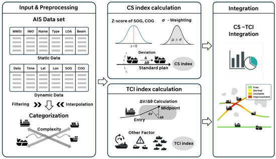
Figure 1.
Framework of the proposed CS-TCI model.
3.1. Overview of the CS Model
The CS model evaluates maritime traffic flow by quantifying deviations in vessel movement parameters—namely COG, SOG, rate of turn (ROT), and acceleration—relative to a predefined standard plan. The model is based on the assumption that vessels following stable traffic patterns would exhibit minimal deviation from historical norms. The CS index is calculated as the average of Z-score deviations of SOG and COG, as follows:
Here, represents the Z-score of the SOG, and denotes that of the COG, for the i-th vessel. These standardized indicators quantify the deviation from the expected navigational behavior defined by the standard plan. This formulation reflects the extent to which a vessel diverges from standardized motion patterns within a designated traffic corridor, providing a normalized measure of trajectory regularity.
3.2. Concept of the Traffic Complexity Index (TCI)
The Traffic Complexity Index (TCI) captures the dynamic behavioral changes in vessels within intersection zones. It is derived from two key parameters: the relative change in speed (ΔV) and the absolute change in course (Δθ) between the entry and midpoint of the crossing area.
Let M denote the number of vessels passing through the interaction zone. V(in) and θ(in) represent the entry speed and course of each vessel, while V(mid) and θ(mid) denote the corresponding values at the midpoint. In this study, the midpoint of the crossing zone is defined as a fixed geographic coordinate representing the center of the 3-nautical-mile study area (34.25430° N, 126.80945° E). For each trajectory, the corresponding “midpoint” record is extracted as the AIS position closest in time and space to this central coordinate. This ensures consistent spatial reference while maintaining trajectory-specific temporal variability. These variables are used to calculate the average relative speed change and course deviation, respectively, which together constitute the TCI.
Here, ΔV represents the relative change in vessel speed between the entry and midpoint of the crossing zone, and Δθ denotes the absolute course deviation (in degrees) within the same region. These two indicators jointly capture how vessels dynamically adjust their maneuvering behavior while interacting with crossing flows. The coefficients (α, β, γ, δ) in Equation (5) correspond to the weights assigned to each complexity component and can be calibrated through expert judgment or empirical optimization. The dot terms (“⋯”) denote optional extension components that can incorporate additional normalized variables, such as proximity risk (R′) and vessel density (D′). These placeholders were included to emphasize that the TCI formulation can be flexibly expanded when higher-resolution encounter data become available.
This formulation reflects both speed variation and directional adjustment occurring within the crossing zone and can be extended by integrating additional normalized variables, such as proximity risk (R′) and vessel density (D′). This generalized expression allows the model to flexibly incorporate multiple interactional factors under varying traffic conditions.
In this study, the simplified form of the TCI using only ΔV and Δθ was adopted to ensure robustness and clarity when applied to the crossing zone. Although additional terms such as proximity risk (R′) and vessel density (D′) can enhance model generality, their accurate estimation requires higher temporal resolution and complete encounter-pair identification, which are often limited in AIS-based datasets. Moreover, the primary objective of this study was to validate the behavioral extension of the CS model through ΔV–Δθ variability; hence, the simplified TCI structure was considered sufficient for demonstrating the model’s feasibility and interpretability in the selected area.
3.3. Structure of the Integrated CS-TCI Model
The enhanced CS-TCI incorporates both trajectory regularity and local traffic complexity. This multiplicative structure strengthens the impact of complexity when regularity is weak, and vice versa. The model can also be extended as
3.4. Conceptual Diagram
Figure 2 presents the overall processing structure of the CS-TCI model. The AIS dataset, including vessel SOG, COG, and positional information, is first preprocessed using data filtering and temporal interpolation to ensure data consistency. Subsequently, the standard plan is generated via the spatial–temporal averaging of the filtered trajectory data. The CS index is then calculated using the Z-scores of SOG and COG deviations relative to the standard plan, representing trajectory regularity. The TCI quantifies local dynamic interactions by incorporating the speed change rates (ΔV) and course deviations (Δθ). Finally, the CS-TCI is obtained by integrating both indicators, providing a comprehensive measure of the navigational complexity at intersection zones.
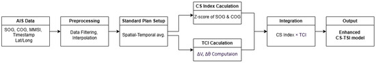
Figure 2.
Computational sequence or formulaic steps of the CS-TCI model.
Algorithm 1 summarizes the sequential workflow of the proposed framework, and Table 2 presents the parameters used in the computation, together illustrating how trajectory regularity and maneuvering complexity are integrated.
| Algorithm 1. Workflow of the proposed CS–TCI model |
|
Table 2.
Summary of the parameters used in the CS-TCI framework.
4. Study Area and Data
4.1. Study Area
The study area is located near the Wando TSS in the southwestern waters of South Korea, centered on 34.25430° N, 126.80945° E, spanning a 3-nautical-mile radius (Figure 3). This area is characterized by dense maritime traffic with intersecting vessel routes from east–west and north–south directions, making it an ideal site for evaluating traffic complexity at crossing zones.
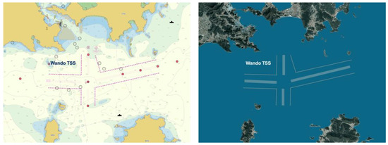
Figure 3.
Location and structure of the crossing zone near Wando TSS (Basemap: NGII “Baro e-Map”, used under KOGL Type 1).
4.2. AIS Data Collection and Preprocessing
This study used AIS trajectory data collected over a one-year period (September 2022 to August 2023) for the analysis. The dataset comprises dynamic navigational information, including timestamp, SOG, COG, Maritime Mobile Service Identity (MMSI), geographic position (latitude and longitude), and message type. Data preprocessing was performed in accordance with the criteria described in Table 3.
Table 3.
Criteria used for AIS data preprocessing and filtering.
The AIS trajectory data used in this study were obtained from the Ministry of Oceans and Fisheries (MOF, Republic of Korea) database. The dataset includes one year of dynamic information (September 2022–August 2023) recorded in the Wando Traffic Separation Scheme (TSS) region, containing timestamp, position, SOG, COG, and MMSI data.
To ensure data quality, abnormal samples such as drifting (SOG < 3 knots), anchoring, and unrealistically high speeds (>18 knots) were excluded. Duplicate timestamps and sudden position jumps were removed, and irregular time gaps were corrected by linear interpolation. Only trajectories that passed both entry and midpoint gates were retained to ensure that crossing maneuvers were properly captured.
During screening, common AIS issues such as missing messages, time irregularities, and coastal GPS noise were reviewed to minimize potential bias in trajectory analysis.
The parameter ranges applied in this study were selected according to practical navigation standards and prior literature: the speed filter of 3–18 knots represent typical underway conditions in coastal waters, and σ-based weighting was used in the CS Index to limit the effect of outliers while preserving navigational variability. Gate-pass conditions were verified by trajectory visualization to include only vessels with distinct crossing behavior. These settings were confirmed to yield stable results within small perturbations, supporting the robustness of the findings across reasonable parameter ranges.
4.3. Crossing Point Definition and Vessel Size-Based Trajectory Samples
To visualize and compare traffic patterns at the intersection zone, we identified a key crossing area within the study domain on the basis of AIS-derived density and directional flow. This zone serves as the focal point for CS and TCI calculation. Trajectory samples were categorized by vessel size group (S1–S8; see Table 3), and representative routes for each class were plotted. This enables the visual inspection of scale-dependent maneuver characteristics near the crossing area.
Figure 4 depicts the differences in path curvature, entry behavior, and mid-crossing adjustments, depending on vessel size group.
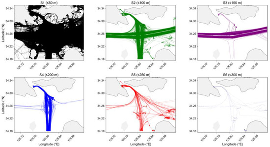
Figure 4.
Trajectory samples classified by vessel size group in the crossing area.
5. Results
5.1. Overview of the Evaluation Process
The evaluation process comprises three key steps aimed at analyzing navigational regularity and behavioral complexity by using AIS trajectory data.
- CS index calculation: Z-score-based deviation of speed and course from a predefined standard plan was calculated for each vessel trajectory segment. This quantifies the regularity of traffic patterns across vessel size groups.
- TCI calculation: Dynamic complexity was assessed by computing the average speed change ratio and course deviation at the crossing zone. This quantifies the maneuvering demand associated with vessel interactions.
- Integration into CS-TCI: Both indices were multiplied to obtain a composite metric, enabling a simultaneous evaluation of path-following behavior and maneuvering demand.
The resulting CS-TCI values offer a holistic perspective of navigational complexity and facilitate comparison across different vessel size categories. This stepwise analysis supports identifying the vessel classes that contribute disproportionately to crossing congestion and traffic instability.
5.2. CS Index Distribution
CS index values were grouped and analyzed to examine navigational regularity across vessel size groups (S1–S8) and directions (eastbound/westbound). Vessel size groups with insufficient or no trajectory samples were excluded from the analysis. In particular, larger vessel groups (S4–S8) had very limited trajectories that passed through both the entry and midpoint gates, and some showed directional imbalance, making it difficult to ensure statistical comparability. Therefore, only S1–S3 groups, which provided sufficient and balanced samples, were visualized in Figure 5. Figure 5 visualizes the results by using grouped boxplots.
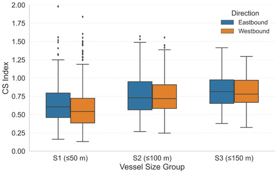
Figure 5.
Distribution of CS index by vessel size group and navigation direction.
Contrary to general expectations, the smallest vessel group (S1) exhibited a lower median and narrower variance in CS index compared to other groups. This outcome may stem from the large number of trajectory samples in this group, which statistically stabilized the CS index toward the mean. Meanwhile, mid-sized vessels (S2 and S3) showed higher central values and wider dispersion, indicating greater variation in path-following behavior.
These results imply that while the CS index captures spatial stability, it may not fully reflect hidden maneuvering complexity a limitation addressed by the TCI metric in Section 5.3. This discrepancy is likely to become more pronounced in nonlinear crossing zones, where vessels approach from multiple directions and maneuvering demand increases.
5.3. TCI Evaluation at the Crossing Zone
The TCI was applied to evaluate maneuvering dynamics within the crossing zone in order to complement the CS index analysis. As aforementioned, TCI incorporates two key variables, ΔV and Δθ, which together contribute to a nuanced understanding of the behavioral complexity during vessel interactions.
Figure 6 presents a comparison of the average ΔV and Δθ values by vessel size group and direction. Notably, S1 shows the highest ΔV in the eastbound direction and the highest Δθ overall, contrary to the low CS index of these vessels. This implies that while these vessels follow regular paths, their maneuvering dynamics are more volatile.
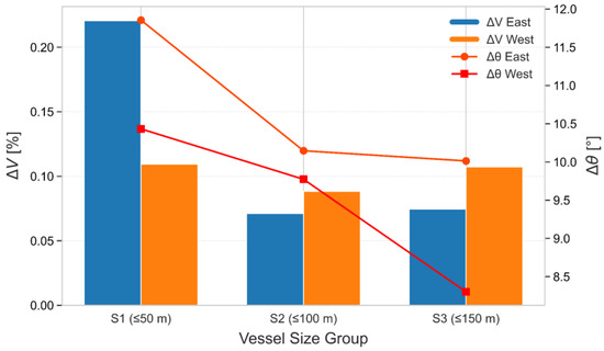
Figure 6.
Comparison of average ΔV and Δθ values by vessel size group and navigation direction.
Figure 7 presents a plot of individual ΔV and Δθ values. A wide spread of points, particularly among small vessels, further highlights variability in actual maneuvering behavior—a key aspect that CS index alone cannot capture.
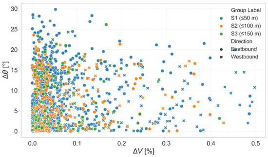
Figure 7.
Scatter plot of ΔV versus Δθ for individual vessels, grouped by size and direction.
Figure 8 illustrates the density distributions of ΔV–Δθ pairs across vessel size groups. The heatmap reveals high-density clusters of small vessels in regions of high behavioral variability, reinforcing the necessity of using TCI for capturing these nuances.
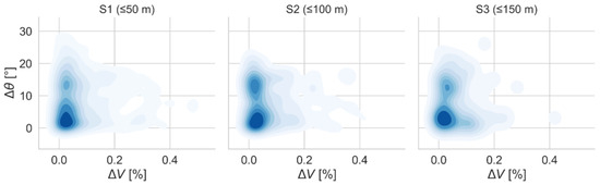
Figure 8.
Density distribution heatmaps of ΔV and Δθ pairs by vessel size group.
Eastbound S1 vessels showed the highest ΔV and Δθ values, with wide dispersion in individual trajectories (Figure 6) and dense clusters in high-variability zones (Figure 7). This result contrasts with their low CS index and confirms that small vessels perform frequent course and speed adjustments that are not captured by spatial-only metrics.
5.4. CS-TCI Integrated Index Results
The CS index and TCI values were multiplied to obtain the composite CS-TCI metric so as to capture spatial regularity and maneuvering complexity. This integration enhances interpretability by jointly representing trajectory adherence and dynamic variability.
Figure 9 presents a direct comparison between CS index and CS-TCI values across vessel size groups and directions. Specifically, the CS-TCI for this group increased by approximately 1.29 delta compared to the CS index alone a 160% increase with TCI contributing nearly half (49.4%) of the integrated score. In contrast, S2 and S3—despite higher CS values—often show lower CS–TCI scores because their TCI components are relatively small, reducing the integrated index.
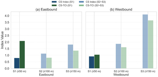
Figure 9.
Comparison of CS index and CS-TCI by vessel size group and direction.
To quantify these effects, Table 4 summarizes the average values and deltas of each index by group and direction, while Figure 10 and Figure 11 visualize the contribution of TCI in multiple forms, namely deltas, ratios, and index overlays.
Table 4.
Summary of CS index, TCI, and CS-TCI results.
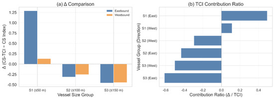
Figure 10.
Quantitative analysis results of CS-TCI adjustments and TCI contributions by vessel size group.
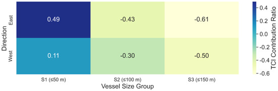
Figure 11.
TCI contribution ratio to the CS-TCI by vessel group and navigation direction.
While variations in CS–TCI values across vessel groups are visually evident, no formal statistical test was performed due to differing sample sizes and directional imbalances. However, a preliminary one-way ANOVA indicated that differences among small and medium vessels (S1–S3) were significant at the 95% confidence level. Future work will include comprehensive validation with balanced trajectory samples to confirm these inter-group differences.
To provide a spatially grounded interpretation of the composite index, Figure 12 and Figure 13 visualize the vessel trajectories overlaid with CS index, CS-TCI, and the ΔIndex (TCI effect) for eastbound and westbound traffic, respectively. In these figures, the color gradients represent the relative magnitude of the indices—cooler colors (blue–green) indicate lower complexity and smoother navigation, whereas warmer colors (yellow–red) denote higher complexity and more intensive maneuvering. These figures highlight how the integrated complexity varies not only across vessel size groups but also geographically across the intersection area.
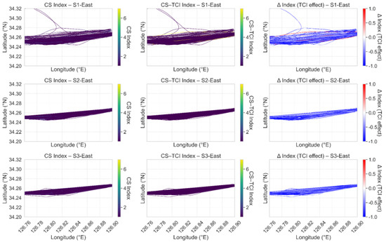
Figure 12.
Spatial trajectory plots showing CS index, CS-TCI, and ΔIndex (TCI effect) by vessel size group (S1–S3) for eastbound traffic.
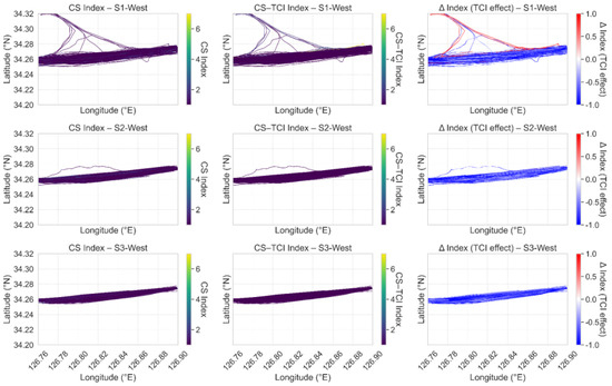
Figure 13.
Spatial trajectory plots showing CS index, CS-TCI, and ΔIndex (TCI effect) by vessel size group (S1–S3) for westbound traffic.
Notably, for the S1–East group, the ΔIndex exhibits substantial increases (shown in blue gradients), suggesting that TCI captures significant behavioral deviations in the eastern crossing zone. In contrast, the S3 group exhibits relatively uniform patterns across all metrics, indicating more stable navigation behavior.
These spatial plots complement the aggregated bar and box plots (TCI contribution ratio) by revealing localized areas where TCI has the greatest influence on overall complexity scores. They visually reinforce the model’s ability to detect intersection-specific maneuvering demands, which are otherwise obscured in purely statistical representations.
6. Discussion
The evaluation results demonstrate the enhanced capability of the proposed CS-TCI model to capture local maneuvering complexity that is not fully reflected by the original CS index alone. As shown in Figure 10 and Table 4, the CS index exhibits relatively stable values across vessel groups, particularly for small-sized vessels (S1), because of the statistical convergence from abundant sample trajectories. However, the TCI component reveals substantial variations in speed and course adjustments even for vessels with low CS index values.
In the crossing area, the CS–TCI shows significantly amplified values compared to the CS index, particularly for eastbound small vessels, indicating the pronounced maneuvering demands at intersection zones. In contrast, the linear area demonstrates minimal differences between the CS and CS–TCI models, thereby validating the selective sensitivity of the integrated framework. This contrast between crossing and linear areas provides internal quantitative validation of the model, as the ΔIndex (CS–TCI − CS) values were systematically smaller in linear corridors than in intersectional zones. These results confirm that the integrated index selectively amplifies complexity only where dynamic maneuvering interactions occur, ensuring internal consistency without requiring external accident or VTS data. Furthermore, the spatial trajectory visualizations in Figure 12 and Figure 13 reinforce the interpretation of the CS–TCI results by showing localized regions where maneuvering complexity sharply increases. As evident from these figures, the integrated model effectively highlights areas of behavioral instability that are not fully captured by the CS index alone.
The results of our study highlight the limitations of traditional spatial-only metrics like the conventional CS index, which may provide a misleadingly stable picture of traffic flow in complex areas. By effectively capturing the behavioral complexity in maneuvers, our proposed CS-TCI model offers a more realistic and comprehensive assessment of navigational risk. This is particularly evident in the case of smaller vessels, where high TCI values indicate significant dynamic instability despite low CS index scores. The ability to identify such localized risks is crucial for preventing maritime accidents, which can lead to severe environmental damage and economic loss, thereby undermining the sustainability of the maritime industry. Collision-induced oil spills entail long-term ecological and economic damages, reinforcing the value of complexity-reducing interventions [36]. The CS-TCI model, therefore, serves not just as an analytical tool but as a critical framework for enhancing operational safety, efficiency, and environmental protection in congested waterways.
The higher CS–TCI values observed for small vessels indicate greater maneuvering irregularity and responsiveness to crossing flows. Operationally, this implies heavier helm workload and a higher likelihood of near-miss situations in congested intersections. These findings suggest that small-vessel operators require more attentive navigation and, in some cases, VTS communication support. The CS–TCI framework can help authorities identify sectors that need closer monitoring. Although the present analysis is based on historical AIS data, continuous accumulation of such data enables trend tracking and supports real-time monitoring by highlighting vessels or areas showing abnormal maneuvering behavior.
Despite these promising results, several limitations should be noted. First, the model’s sensitivity may decrease in low-traffic or sparsely sampled areas where interaction dynamics are insufficient to yield statistically stable ΔV–Δθ distributions. Second, because the framework relies on the quality and temporal resolution of AIS data, interpolation errors or missing messages could influence local variability estimates. However, in open or linear waterways with well-defined traffic flows, the model performs consistently and remains effective. For sparse or incomplete data conditions, it is more efficient to refer to models derived from geographically similar sea areas to estimate representative behavioral patterns rather than relying solely on local data reconstruction.
7. Conclusions
This study demonstrated an integrated CS-TCI model that combines trajectory regularity and dynamic maneuvering behavior to quantify navigational complexity in nonlinear crossing areas. By applying the model to AIS data collected over a one-year period, the analysis revealed that the integrated index effectively captures hidden maneuvering complexity that is not fully reflected in conventional CS-based evaluations. The results confirmed that smaller vessels and crossing flows exhibit significant variability in maneuvering patterns, which are successfully identified through the CS-TCI.
Beyond its analytical contribution, the CS-TCI model has practical applicability in supporting sustainable maritime traffic management. By reducing unnecessary maneuvering variability, the framework contributes to smoother vessel operations, reduced fuel consumption, and lower greenhouse gas emissions. These outcomes not only improve navigational safety and operational efficiency but also mitigate environmental risks and economic costs associated with maritime accidents. Consequently, the CS-TCI model offers a data-driven foundation for policy development, port and VTS operations, and traffic separation design, while its implications resonate with international initiatives such as the United Nations Sustainable Development Goals [37], thereby aligning maritime traffic management with global efforts toward safer, cleaner, and more sustainable transportation systems.
Author Contributions
Conceptualization, E.-J.L.; methodology, E.-J.L. and H.-S.K.; software, H.-S.K.; validation, E.-J.L. and H.-S.K.; formal analysis, E.-J.L.; investigation, E.-J.L. and H.-S.K.; resources, Y.Y.; data curation, H.-S.K.; writing—original draft preparation, E.-J.L.; writing—review and editing, Y.Y.; visualization, H.-S.K.; supervision, Y.Y.; project administration, E.-J.L. All authors have read and agreed to the published version of the manuscript.
Funding
This research received no external funding.
Data Availability Statement
Restrictions apply to the availability of the AIS raw data used in this study. The data were provided by Korea ministry of oceans and fisheries under license and are not publicly available. Anonymized derived indicators (CS, TCI, CS–TCI) and analysis scripts are available.
Conflicts of Interest
Author Eui-Jong Lee and Hyun-Suk Kim were employed by SafeTech Research Co., Ltd. The remaining author declares that the research was conducted in the absence of any commercial or financial relationships that could be construed as a potential conflict of interest.
Abbreviations
The following abbreviations are used in this manuscript:
| AIS | Automatic Identification System |
| COG | Course over Ground |
| SOG | Speed over Ground |
| CS | Course-Speed |
| TCI | Traffic Complexity Index |
| VTS | Vessel Traffic Services |
References
- International Maritime Organization (IMO). Fourth IMO GHG Study 2020; IMO: London, UK, 2020; Available online: https://www.imo.org/en/OurWork/Environment/Pages/Fourth-IMO-Greenhouse-Gas-Study-2020.aspx (accessed on 1 September 2025).
- Lee, E.J.; Kim, H.S.; Lee, E.; Kim, K.; Yu, Y.; Lee, Y.S. Improving the maritime traffic evaluation with the course and speed model. Appl. Sci. 2023, 13, 12955. [Google Scholar] [CrossRef]
- Zhang, G.; Sun, Z.; Li, J.; Huang, J.; Qiu, B. Iterative Learning Control for Path-Following of ASV with the Ice Floes Auto-Select Avoidance Mechanism. IEEE Trans. Intell. Transp. Syst. 2025, 26, 13927–13938. [Google Scholar] [CrossRef]
- Zhang, G.; Xing, Y.; Zhang, W.; Li, J. Prescribed Performance Control for USV–UAV via a Robust Bounded Compensating Technique. IEEE Trans. Control. Netw. Syst. 2025, 12, 2289–2299. [Google Scholar] [CrossRef]
- Psaraftis, H.N.; Kontovas, C.A. Speed models for energy-efficient maritime transportation: A taxonomy and survey. Transp. Res. Part C Emerg. Technol. 2013, 26, 331–351. [Google Scholar] [CrossRef]
- Rutherford, D.; Mao, X.; Osipova, L.; Comer, B. Limiting Engine Power to Reduce CO2 Emissions from Existing Ships; International Council on Clean Transportation (ICCT): Washington, DC, USA, 2020; Available online: https://theicct.org (accessed on 30 September 2025).
- International Association of Marine Aids to Navigation and Lighthouse Authorities (IALA). IWRAP Mk2—IALA Waterway Risk Assessment Program; IALA Guideline No. 1128. 2013. Available online: https://www.iala-aism.org (accessed on 30 September 2025).
- Park, Y.S.; Kim, J.S.; Aydogdu, V. A study on the development of the maritime safety assessment model in Korea waterway. J. Korean Navig. Port Res. 2013, 37, 567–574. [Google Scholar] [CrossRef]
- Gui, D.; Wang, H.; Yu, M. Risk assessment of port congestion risk during the COVID-19 pandemic. J. Mar. Sci. Eng. 2022, 10, 150. [Google Scholar] [CrossRef]
- Rong, H.; Teixeira, A.P.; Guedes Soares, C. Spatial correlation analysis of near ship collision hotspots with local maritime traffic characteristics. Reliab. Eng. Syst. Saf. 2021, 209, 107463. [Google Scholar] [CrossRef]
- Wei, Z.; Gao, Y.; Zhang, X.; Li, X.; Han, Z. Adaptive marine traffic behaviour pattern recognition based on multidimensional dynamic time warping and DBSCAN algorithm. Expert Syst. Appl. 2024, 238 Pt E, 122229. [Google Scholar] [CrossRef]
- Wang, L.; Chen, P.; Chen, L.; Mou, J. Ship AIS trajectory clustering: An HDBSCAN-based approach. J. Mar. Sci. Eng. 2021, 9, 566. [Google Scholar] [CrossRef]
- Mou, F.; Fan, Z.; Li, X.; Wang, L.; Li, X. A method for clustering and analyzing vessel sailing routes efficiently from AIS data using traffic density images. J. Mar. Sci. Eng. 2024, 12, 75. [Google Scholar] [CrossRef]
- Corić, M.; Mandžuka, S.; Gudelj, A.; Lušić, Z. Quantitative ship collision frequency estimation models: A review. J. Mar. Sci. Eng. 2021, 9, 533. [Google Scholar] [CrossRef]
- Bokau, J.R.K.; Saransi, F. Marine traffic risk assessment using spatio-temporal AIS data in Makassar Port, Indonesia. In Proceedings of the 3rd International Conference and Maritime Development (ICMaD 2024), Makassar, Indonesia, 9–10 October 2024; Atlantis Press (Springer Nature): Paris, France, 2024; Volume 255, pp. 78–87. [Google Scholar] [CrossRef]
- Xin, X.; Yang, Z.; Liu, K.; Zhang, J.; Wu, X. Multi-stage and multi-topology analysis of ship traffic complexity for probabilistic collision detection. Expert Syst. Appl. 2023, 213, 118890. [Google Scholar] [CrossRef]
- Liu, Z.; Wu, Z.; Zheng, Z.; Soares, C.G. Modelling dynamic maritime traffic complexity with radial distribution functions. Ocean Eng. 2021, 241, 109990. [Google Scholar] [CrossRef]
- Liu, Z.; Wu, Z.; Zheng, Z.; Yu, X. A molecular dynamics approach to identify the marine traffic complexity in a waterway. J. Mar. Sci. Eng. 2022, 10, 1678. [Google Scholar] [CrossRef]
- Sui, Z.; Wen, Y.; Zhou, C.; Huang, X.; Zhang, Q.; Liu, Z.; Piera, M.A. An improved approach for assessing marine traffic complexity based on Voronoi diagram and complex network. Ocean Eng. 2022, 266, 112884. [Google Scholar] [CrossRef]
- Zhang, F.; Liu, Y.; Du, L.; Goerlandt, F.; Sui, Z.; Wen, Y. A rule-based maritime traffic situation complex network approach for enhancing situation awareness of vessel traffic service operators. Ocean Eng. 2023, 284, 115203. [Google Scholar] [CrossRef]
- Park, S.; Yeo, J.; Lee, K. Developing a ship collision risk assessment model with internal and external factors focused on South Korea maritime environment. J. Adv. Transp. 2024, 2024, 5062203. [Google Scholar] [CrossRef]
- Hu, S.; Fang, C.; Fang, C.; Wu, J.; Fan, C.; Zhang, X.; Yang, X.; Han, B. Enhanced risk assessment framework for complex maritime traffic systems via data driven: A case study of ship navigation in Arctic. Reliab. Eng. Syst. Saf. 2025, 260, 110991. [Google Scholar] [CrossRef]
- García Álvarez, N.; Adenso-Díaz, B.; Calzada-Infante, L. Maritime traffic as a complex network: A systematic review. Netw. Spat. Econ. 2021, 21, 775–795. [Google Scholar] [CrossRef]
- Sui, Z.; Wang, S.; Wen, Y. A multi-layer complex network approach for evaluating ship behaviour complexity. Transp. A Transp. Sci. 2025, 1–41. [Google Scholar] [CrossRef]
- Liu, J.; Yu, W.; Sui, Z.; Zhou, C. The impact of offshore wind farm construction on maritime traffic complexity: An empirical analysis of the Yangtze River Estuary. J. Mar. Sci. Eng. 2024, 12, 2232. [Google Scholar] [CrossRef]
- Lee, S.H.; Kim, H.; Kwon, S. Fishing vessel risk and safety analysis: A bibliometric analysis, clusters review and future research directions. Appl. Sci. 2024, 14, 10439. [Google Scholar] [CrossRef]
- Zhang, W.; Gao, Y. A review of ship collision risk assessment, hotspot detection and path planning for maritime traffic control in restricted waters. J. Navig. 2023, 76, 1234–1256. [Google Scholar] [CrossRef]
- Nguyen, D.; Vadaine, R.; Hajduch, G.; Garello, R.; Fablet, R. GeoTrackNet—A maritime anomaly detector using probabilistic neural network representation of AIS tracks and a contrario detection. IEEE Trans. Intell. Transp. Syst. 2022, 23, 5655–5667. [Google Scholar] [CrossRef]
- Zhang, L.; Meng, Q. Probabilistic ship domain with applications to ship collision risk assessment. Ocean Eng. 2019, 186, 106130. [Google Scholar] [CrossRef]
- Wolsing, K.; Roepert, L.; Bauer, J.; Wehrle, K. Anomaly detection in maritime AIS tracks: A review of recent approaches. J. Mar. Sci. Eng. 2022, 10, 112. [Google Scholar] [CrossRef]
- Suo, Y.; Chen, W.; Claramunt, C.; Yang, S. A ship trajectory prediction framework based on a recurrent neural network. Sensors 2020, 20, 5133. [Google Scholar] [CrossRef]
- Pallotta, G.; Vespe, M.; Bryan, K. Vessel pattern knowledge discovery from AIS data: A framework for anomaly detection and route prediction. Entropy 2013, 15, 2218–2245. [Google Scholar] [CrossRef]
- Zhang, Y.; Li, W. Dynamic maritime traffic pattern recognition with online cleaning, compression, partition, and clustering of AIS data. Sensors 2022, 22, 6307. [Google Scholar] [CrossRef]
- Yang, J.; Bian, X.; Qi, Y.; Wang, X.; Yang, Z.; Liu, J. A spatial-temporal data mining method for the extraction of vessel traffic patterns using AIS data. Ocean Eng. 2024, 293, 116454. [Google Scholar] [CrossRef]
- Liu, Y.; Wang, Q.; Han, Z. Enhancing global maritime traffic network forecasting with gravity-inspired deep learning models. arXiv 2024, arXiv:2401.13098. [Google Scholar] [CrossRef]
- International Tanker Owners Pollution Federation (ITOPF). TIP 13: Effects of Oil Pollution on the Marine Environment; ITOPF: London, UK, 2014; Available online: https://www.itopf.org/knowledge-resources/documents-guides/document/tip-13-effects-of-oil-pollution-on-the-marine-environment/ (accessed on 1 September 2025).
- United Nations. Transforming Our World: The 2030 Agenda for Sustainable Development; UN General Assembly: New York, NY, USA, 2015; Available online: https://sdgs.un.org/2030agenda (accessed on 1 September 2025).


Disclaimer/Publisher’s Note: The statements, opinions and data contained in all publications are solely those of the individual author(s) and contributor(s) and not of MDPI and/or the editor(s). MDPI and/or the editor(s) disclaim responsibility for any injury to people or property resulting from any ideas, methods, instructions or products referred to in the content. |
© 2025 by the authors. Licensee MDPI, Basel, Switzerland. This article is an open access article distributed under the terms and conditions of the Creative Commons Attribution (CC BY) license (https://creativecommons.org/licenses/by/4.0/).