Hybrid Log-Mel and HPSS-Aided Convolutional Neural Network for Underwater Very-Low-Frequency Remote Passive Sonar Detection

Abstract

Very-low-frequency (VLF) passive sonar detection is one of the core technologies for maritime surveillance, although its performance is often severely affected by strong impulsive ocean ambient noise interference. This paper, for the first time, proposes a convolutional neural network (CNN) detection framework with hybrid Log-Mel spectrogram (Log-Mel) and Harmonic–Percussive Source Separation (HPSS) preprocessing. Aiming to highlight the detailed features of low frequencies in accordance with impulsive noise interference removal, the network was trained on a measured dataset in the South China Sea for a whole week by maximize the area under receiver operating characteristic curve (AUC) that corresponds to a false alarm probability of less than 0.1. The test results show that compared with a typical Short-Time Fourier Transform (STFT) input feature, the utilization of Log-Mel and HPSS can be superior, especially utilizing Log-Mel and HPSS(H) features at the same time. Validation with a set of measured moving ship data shows that the detection performance of the proposed hybrid Log-Mel and HPSS-aided CNN can be stable and significantly improve the remote passive sonar detection performance.

1. Introduction

The passive sonar detection of underwater targets is one of the key technologies for maritime surveillance and ocean engineering, particularly in the very-low-frequency (VLF) band [1]. Unlike active sonar, which releases acoustic pulses and listens for returning echoes, passive sonar relies only on the receipt of ship-radiated or submarine-radiated sounds. This makes passive sonar inherently stealthier and indispensable for naval defense, anti-submarine warfare, and long-term ocean monitoring [2,3]. Using experiments and modeling, an excellent description of ship-radiated noise had been given as a combination of broadband noise and line spectral signatures [4,5,6]. These line spectral fingerprints correspond to the rotation of engines, shaft-line dynamics, propeller cavitations which are usually applied to various algorithms for passive sonar detection, tracking, and classification.

However, the performance of VLF passive sonar detection is strongly hampered by the features of ocean noise, which are often non-Gaussian, extremely non-stationary, and highly variable in time and space [7]. Plenty of experimental and modeling studies have revealed that the underwater acoustic noise environment is non-Gaussian and impulsive in nature [8,9,10,11]. Typical modeling approaches include Gaussian Mixture (GM) [12], Generalized Gaussian Distribution (GG) [13], $\alpha$ stable distribution model (S$\alpha$S) [14], etc. For typical measured maritime ambient noise, there is a considerable amount of strong random impulsive interference, mainly in the form of energy distributed in the lower frequency. In this way, classical detection methods are effective in relatively simple acoustic environments in the higher frequency band (>100 Hz), but struggle against modern challenges in the very-low-frequency band (<100 Hz) of shipping traffic, and highly dynamic natural noise from wind, waves and marine life [15,16]. Moreover, the Gaussianity assumption no longer matches the statistical features of real underwater environments, resulting in a sub-optimal performance or worse [17,18,19].

As is known for non-Gaussian signal detection, an optimal receiving method for signal detection is to construct nonlinear filters to approach the optimal nonlinear transfer function [20]. These indicate that detection theories and methods under non-Gaussian noise should be nonlinear. On the basis of this, nonlinear methods generally adopted for weak signal detection, such as chaos-based methods [21], stochastic resonance [2,22,23], higher-order statistics [24], and fractal dimension analysis [25], have been applied to better deal with non-Gaussian noise. However, the optimal nonlinear systems frequently have complex architectures. The aforementioned nonlinear method cannot approximate the optimal nonlinear transfer function in general, where more complex nonlinear sysytems are adopted for potential performance enhancement [26]. In recent years, the rapid advancement of deep learning has provided new opportunities for sonar signal analysis. Deep neural networks can automatically learn hierarchical features from raw or transformed acoustic signals, removing the need for handcrafted feature engineering [27]. Convolutional Neural Networks (CNNs), in particular, are well suited for sonar detection, as spectrograms of acoustic signals can be treated as two-dimensional images [28]. CNNs have proven significant skills in extracting discriminative time–frequency patterns, robustly handling noise, and generalizing across multiple environments [29]. Several recent studies have highlighted the success of CNNs in underwater acoustics [30]. For instance, CNNs trained on Log-Mel spectrogram features have shown a higher performance in classifying ship-radiated noise, leveraging the Mel scale’s ability to emphasize perceptually important low-frequency bands [31]. Hybrid models combining CNNs with recurrent networks, such as CNN-LSTM frameworks, have further improved classification by modeling both spatial and temporal dynamics [32]. Attention-based CNNs and adaptive filter architectures have also emerged, showing resilience to environmental variability and enabling finer-grained spectral feature learning [33]. To enhance the feature design of CNN input, Harmonic–Percussive Source Separation (HPSS) was adopted for sonar signal analysis. It can decompose spectrograms into harmonic components (stable tonal structures) and percussive components (transient broadband structures). As a result, it can effectively remove impulsive noise interference and retain the tonal features of ship-radiated noise when applied to underwater signals, thereby improving the detectability of moving ships [34,35]. These advancements firmly establish CNNs as a powerful tool for sonar detection, but their performance is ultimately dependent on the quality of the input features, especially under the very-low-frequency band with non-Gaussian impulsive background noise.

Motivated by the aforementioned studies, a compelling solution develops from hybrid feature design. By combining Log-Mel spectrograms and HPSS harmonic features, one can use both perceptually meaningful low-frequency energy distributions and stable harmonic structures contained within the noise. Log-Mel spectrograms emphasize the low-frequency bands important for VLF sonar, whereas HPSS harmonics provide robustness against transient and wideband disturbances. By relying on this insight, the present study offers a hybrid Log-Mel and HPSS-aided CNN framework for VLF passive sonar detection. The key contributions are threefold:

(1) A systematic non-Gaussian statistical analysis of deep sea VLF ocean noise is given with a week-long noise dataset.

(2) A hybrid Log-Mel and HPSS feature-aided deep CNN detection framework is designed, aiming to highlight the detailed features of low frequencies in accordance with impulsive noise interferences removal.

(3) A 10-layer optimal CNN was trained and tested with hybrid features and comprehensively compared against conventional STFT, Log-Mel, and HPSS, which can demonstrate its superior performance with experimental verification.

(4) This study can offer a robust solution to the long-standing challenges of VLF remote passive sonar detection, especially under non-Gaussian impulsive background noise.

The rest of the paper is organized as follows. Section 2 describes the construction of the training and test datasets, and gives a comprehensive non-Gaussian characteristics analysis of deep sea very-low-frequency ambient noise. In Section 3, the hybrid Log-Mel and HPSS feature-aided deep CNN detection framework is given, and a 10-layer optimal CNN is trained and tested with hybrid features. In Section 4, the detection performance is verified with a designed deep sea experiment in the South China Sea, where a moving ship first passed abeam and moved away, which can demonstrate the superior detection performance of the proposed method. Section 5 presents the discussions. Finally, Section 6 presents the conclusions.

2. Dataset and Analysis

This section analyzes an eight-day continuous navigation experimental dataset, partitions the collected signals, and applies time–frequency analysis methods to investigate both ship-radiated noise and ocean ambient noise.

2.1. Dataset Overview

The dataset employed in this study was obtained from an eight-day intermittent navigation and sea trial conducted by a vessel in the South China Sea. A total of 165.67 h of acoustic data were collected during the trial. The receiving hydrophone was deployed at a depth of approximately 1700 m, and the sound pressure channel data from the vector hydrophone were selected as the experimental input for the passive detection of underwater targets.

2.2. Overall Experimental Process

During the eight-day sea trial, the test vessel conducted reciprocal navigation around the receiving hydrophone X. A total of 994 data files were collected by the hydrophone, each representing a 10 min segment. Based on the experimental log, a navigation record table was compiled, as shown in

Table 1. Dataset of ship navigation distance log.

Serial Number	File Name	Distance to Hydrophone X (km)	Signal Presence (0 for No, 1 for Yes)	Strong Impulsive Presence (0 for No, 1 for Yes)
1	0516083849	27	1	0
2	0516084849	27.314	1	0
3	0516085849	26	1	0
4	0516090849	29	1	0
…	…	…	…	…
50	0516164849	9	1	0
51	0516165849	9.5	1	0
…	…	…	…	…
110	0517020849	56	0	0
111	0517021849	56	0	0
…	…	…	…	…
220	0518074849	140	1	1
221	0518080849	138	1	1
…	…	…	…

. The file names correspond to the start time of each recorded segment and represent the subsequent 10 min of hydrophone data. The table also documents the vessel’s operational status: a value of 1 indicates that the vessel was underway, whereas 0 indicates that it was drifting with the engine shut down. In addition, the experimental log annotates the presence of external interference, where a value of 1 indicates interference and a value of 0 indicates no interference. Using this navigation record, the trajectory of the test vessel was reconstructed, as illustrated in Figure 1.

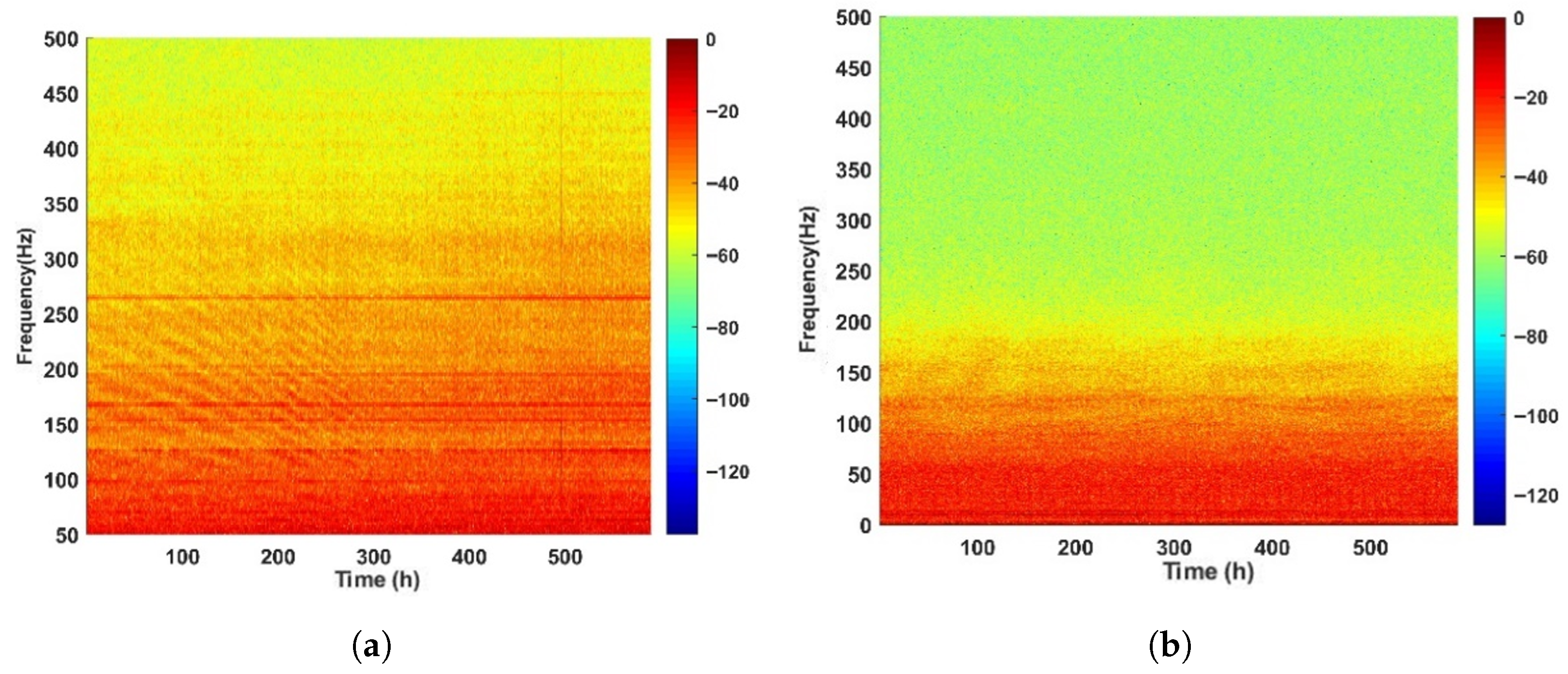
Figure 2a,b present the time–frequency plots of ship-radiated noise and ocean environmental noise, respectively. These plots clearly demonstrate the substantial differences between ship-radiated noise and ocean environmental noise in the time–frequency domain. In Figure 2a, which corresponds to the time–frequency plot during a beamwise pass, ship-radiated noise exhibits distinct line spectra, harmonic components, and acoustic signatures. In particular, within the 50–350 Hz range, clear line spectral components are observed, with the most prominent line spectrum located around 250 Hz, accompanied by multiple modulated line spectra. This plot corresponds to the vessel’s approach toward hydrophone X, where a clear acoustic signature is evident. In contrast, Figure 2b shows that the energy of ocean environmental noise is primarily concentrated below 100 Hz, with no discernible patterns or regularities.

2.3. Dataset Division

To facilitate subsequent analyses, a threshold distance of 30 km was adopted as the criterion for dividing the data into Sample 1 (signal) and Sample 0 (noise). The labeling criteria for both categories are summarized in

Table 2. Sample labeling criteria.

Category	Labeling Criteria	Number of Samples
Sample ‘1’ (Signal)	<30 km ship-radiated noise	48
Sample ‘0’ (Noise)	>30 km ship-radiated noise or ocean environmental noise	946

, and this classification was employed to determine the presence or absence of a signal.

According to the aforementioned classification criteria, 48 samples were labeled as “1” (signal), whereas 946 samples were labeled as “0” (noise). A subset of the samples also contained additional interference.

The acoustic signals acquired by the hydrophone exhibit pronounced non-stationarity and temporal variability. To enhance signal quality for subsequent feature extraction, several preprocessing steps were applied, including DC removal, normalization, framing with windowing (20 s observation windows with a 10 s overlap), and data augmentation. These procedures yielded higher-quality acoustic signal segments of ship-radiated noise and ocean ambient noise, making them more suitable for further analysis.

As noted in Section 2.3 (Dataset Division), the dataset suffers from an imbalance between ship-radiated noise and ocean background noise, with the number of noise samples substantially exceeding that of signal samples. During training, this imbalance introduces bias toward the majority class, thereby degrading network performance. Furthermore, due to confidentiality constraints, acquiring ship-radiated noise samples is costly. Prior work has demonstrated that data augmentation can significantly improve the performance of neural networks under such conditions.

For this study, the data collected from 20:00 on 16 May to 00:00 on 17 May were used as continuous navigation test data for the network, while the remaining data were framed, windowed, and augmented. All processed data were stored in .mat format files. In total, 46,580 signal samples and 45,300 noise samples were generated. These two categories were then combined and randomly partitioned into training, validation, and test sets using a 7:2:1 ratio. The training set was employed to optimize the model, the validation set was used to adjust hyperparameters and conduct preliminary evaluations, and the test set was used to assess the model’s generalization capability. The detailed data division is provided in

Table 3. Passive underwater target detection dataset division.

Category	Total Data Volume	Training Set (70%)	Validation Set (20%)	Test Set (10%)
Signal	46,580	32,606	9316	4658
Noise	45,300	31,710	9060	4530
Total data volume	91,880	64,316	18,376	9188

.

2.4. Non-Gaussian Characteristics Analysis of Deep Sea Very-Low-Frequency Ambient Noise

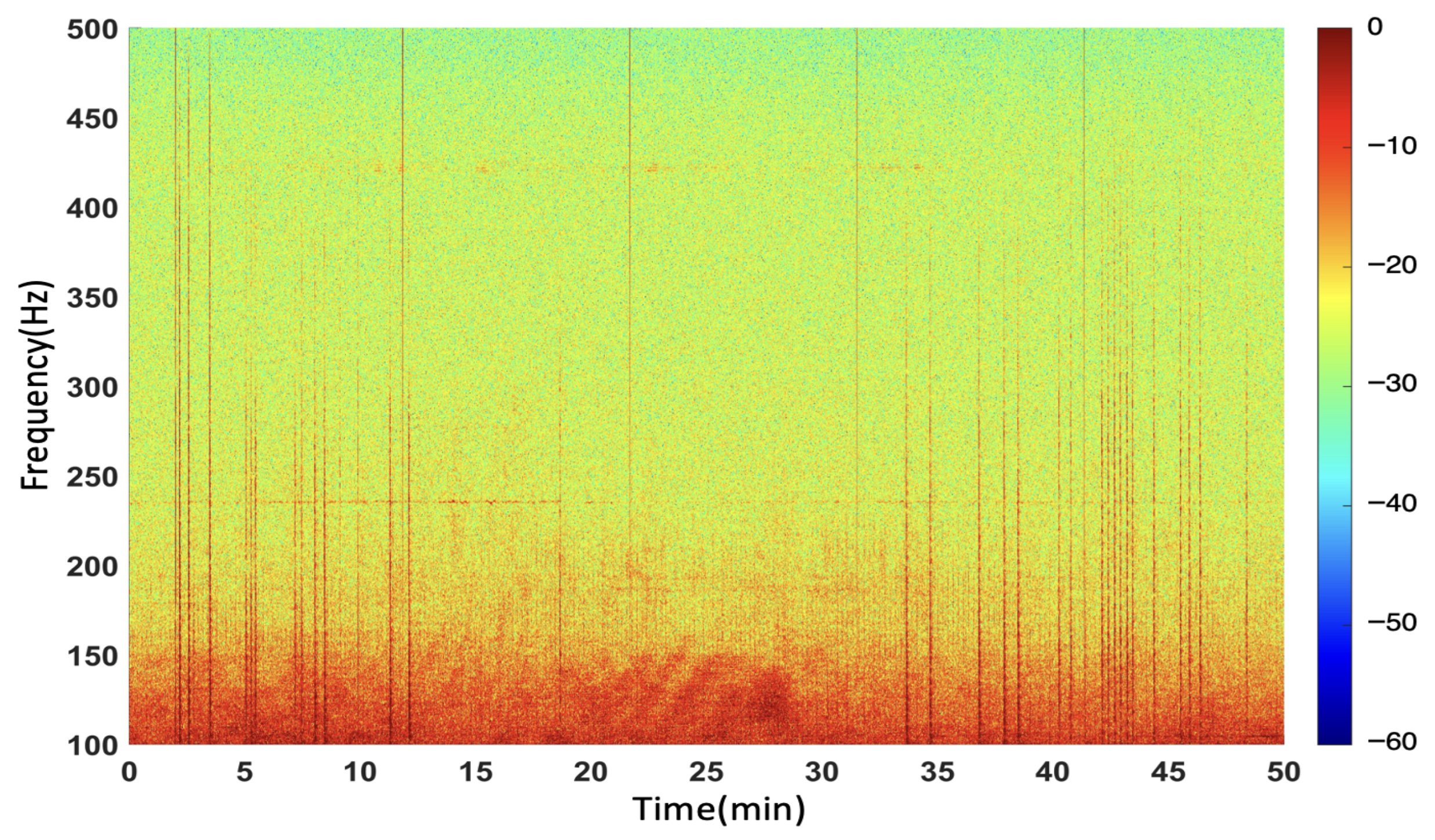
The deep sea environmental noise dataset was collected during a very-low-frequency acoustic sensing experiment conducted in the Dongsha area of the South China Sea. Figure 3 shows a set of 50 min time–frequency maps of typical measured marine ambient noise in the South China Sea. It can be seen that there is a large amount of strong random impulsive interference, mainly energy distributed in the lower frequency, below 100 Hz.

To eliminate the influence of passing vessels in close proximity, all data segments containing noticeable ship passages were carefully excluded. A total of 30 segments, amounting to 3990 min of continuous recordings, were selected to construct the dataset. The key information of each segment is summarized in

Table 4. VLF-UAVS recording sessions.

ID	Date	Time	Channels	Duration (min)	Airgun Pulse Interference
1	5.16	10:18–11:18	4	60	No
2	5.16	13:08–15:08	4	120	No
3	5.16	22:50–23:59	4	69	No
…	…	…	…	…	…
11	5.18	16:00–19:00	4	180	Yes
12	5.18	21:00–22:00	4	60	Yes
13	5.19	03:00–06:00	4	180	Yes
…	…	…	…	…	…
26	5.21	18:00–19:00	4	60	Yes
27	5.21	21:00–23:30	4	150	No

.

When extracting the dataset, both daylight (06:00–20:00) and evening (20:00–06:00) intervals were investigated to account for anticipated diurnal fluctuations in noise characteristics. During the experimental period (18–21 May), the South China Sea region was continuously influenced by strong impulsive sources such as seismic airguns and deep water blasting operations from petroleum exploration and scientific surveys. These impulsive signals, with repetition times ranging from seconds to minutes, constituted approximately half of the dataset. This illustrates the considerable impact of anthropogenic impulsive interference on the deep sea acoustic environment. Accordingly, Table 4 explicitly states whether each data segment has airgun pulse interference.

A non-Gaussian impulsive analysis was performed on the ocean environmental noise dataset acquired by the very-low-frequency (VLF) vector hydrophone between 16 and 22 May. An observation window of 20 s with a 10 s overlap was chosen for continuous analysis. Although the dispersion and symmetry of the noise can be defined by the mean and variance, the amplitude distribution during large sample averaging and signal preprocessing remains unbiased and symmetric. Since the lower-order moments of stable distributions are bounded, parameter estimation can be performed using fractional lower-order moments or logarithmic moment estimation. Considering the advantages of the logarithmic moment estimation method, this study employs this method to estimate the parameters of the recorded very-low-frequency ocean ambient noise. For this purpose, the following section discusses the theoretical framework and estimation approach applied for parameter extraction based on the logarithmic moment method.

In order to represent the actual deep sea ambient noise using the Lévy distribution, it is necessary to estimate the four parameters of the distribution using collected data. However, since the Lévy distribution does not possess a closed-form probability density function, typical statistical approaches based on explicit density representations cannot be utilized. Moreover, its higher-order, and even second-order, statistical moments do not exist. To circumvent this constraint, the concept of fractional lower-order moments (FLOMs) is developed. Based on the logarithmic moment approach, the parameters of the Lévy distribution for genuine low-frequency oceanic ambient noise can be determined. The relationship between FLOMs and the characteristic exponent $\alpha$ as well as the dispersion parameter $\gamma$ in the characteristic function is provided by

$${E\left(\right|X|}^p)=C(p,\alpha ){\gamma }^{p/\alpha },-1<p<\alpha <2$$

(1)

where

$$C(p,\alpha )={\displaystyle \frac{2^{p+1}\Gamma \left(\frac{p+1}{2}\right)\Gamma \left(-\frac{p}{\alpha }\right)}{\alpha \sqrt{\pi }\Gamma \left(-\frac{p}{2}\right)}}.$$

Let $Y=log\left|X\right|$. If a random variable X satisfies $E\left(Y\right)=E(log|X\left|\right)<\infty$, then X is referred to as a log-moment random variable. Its moment-generating function is defined as

$${E\left[\right|X|}^n]=\underset{p\to 0}{lim}{\displaystyle \frac{d^n}{d{p}^n}}\left(E\left[\right|X{|}^p]\right),n=1,2,\dots \dots$$

(2)

Thus, the Lévy distribution possesses finite log-moments, and the second- and higher-order log-moments of Y are determined solely by the characteristic exponent $\alpha$ as follows:

$$\left\{\begin{array}{c}{L}_1=E[log|X\left|\right]={\psi }_0(1-\frac{1}{\alpha })+\frac{1}{\alpha }log|\frac{\sigma }{cos\theta }|\hfill \\ L_2=E\left[(log|X|-{E[log|X\left|\right])}^2\right]={\psi }_1\left(\frac{1}{2}+\frac{1}{{\alpha }^2}\right)-\frac{{\theta }^2}{{\alpha }^2}\hfill \\ L_3=E\left[(log|X|-{E[log|X\left|\right])}^3\right]={\psi }_2\left(1-\frac{1}{{\alpha }^3}\right)\hfill \end{array}\right.$$

(3)

where ${\psi }_{i-1}={\left.{\displaystyle \frac{d^i}{d{x}^i}}log\Gamma \left(x\right)\right|}_{x=1}$, with ${\psi }_0=-0.57721566$, ${\psi }_1=\frac{{\pi }^2}{6}$, and ${\psi }_2=1.2020569$.

Since higher-order log-moment estimations are generally wrong, only the first and second log-moments are typically applied to estimate the parameters of the Lévy distribution. It is typically considered that underwater ambient noise is unbiased with a location parameter of zero. The main focus is consequently on the noise intensity, which is defined by the characteristic exponent $\alpha$ and the scale parameter $\sigma$. Their estimates are obtained using the following formulas:

$$\widehat{\alpha }={\left({\displaystyle \frac{L_2}{{\psi }_1}}-{\displaystyle \frac{1}{2}}\right)}^{-{\displaystyle \frac{1}{2}}}$$

(4)

$$|\widehat{\theta }|={\left(\left({\displaystyle \frac{{\psi }_1}{2}}-L_2\right){\widehat{\alpha }}^2-{\psi }_1\right)}^{{\displaystyle \frac{1}{2}}}$$

(5)

$$\widehat{\sigma }=cos\left(\widehat{\theta }\right)exp\left((L_1-{\psi }_0)\widehat{\alpha }+1\right)$$

(6)

To verify the efficiency of this estimation approach, Lévy noise with $\alpha =1.5$ and $\sigma =1$ was created using the Janicki–Weron algorithm, and the parameters were subsequently estimated using the logarithmic moment method.

Accordingly, the analysis focuses on the impulsive and heavy-tailed features of the data, represented by fluctuations in the characteristic exponent $\alpha$. The results from the P-channel data are shown in Figure 4, which illustrate that deep sea ambient noise exhibits sparse, strong impulsive, non-Gaussian behavior on the minute scale. In most cases, $\alpha >1.8$, but severe impulsive interferences exist. Values of $\alpha <1.8$ are primarily connected to seismic sources, such as airgun transmissions. $\alpha =2$ represents Gaussian values.Although such events occur infrequently, they drastically affect the noise backdrop and underline the intrinsic complexity of the marine auditory environment.

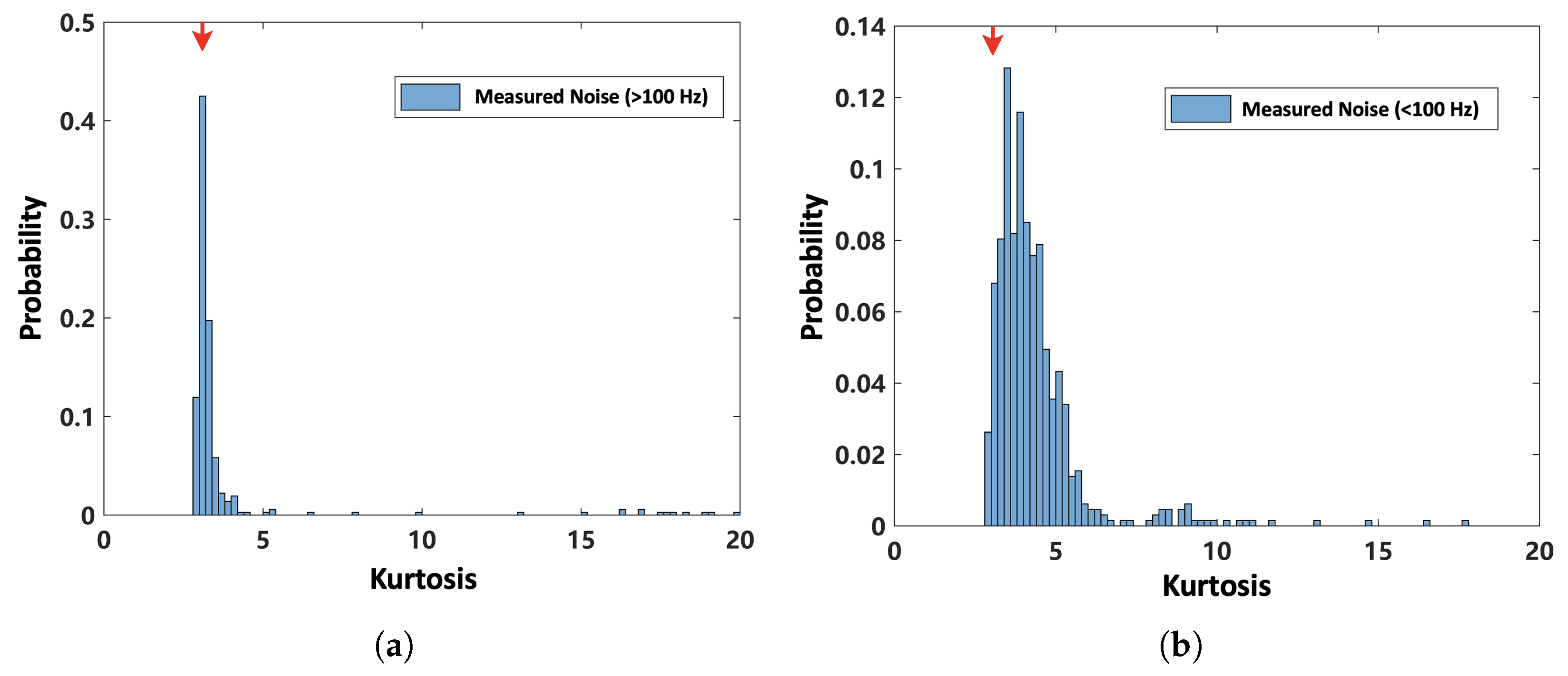
To further validate these observations, the kurtosis distributions of noise segments in the frequency bands above 100 Hz and below 100 Hz were investigated, as shown in Figure 5a,b. This study reveals that while most segments display modest kurtosis values, a large number of outliers with extremely high values are also present, thus indicating the highly impulsive nature of the observed ambient noise. The red arrow represent Gaussian noise.

In summary, the experimental results reveal that deep sea ambient noise is not only non-Gaussian but also highly impulsive and changeable, offering considerable problems for underwater detecting systems. Conventional feature extraction algorithms struggle to properly capture these properties. In contrast, the Log-Mel spectrogram provides robustness against impulsive distortions through logarithmic compression, and HPSS (Harmonic–Percussive Source Separation) separates harmonic and transient components to emphasize organized signal information. Accordingly, the combined use of Log-Mel and HPSS features is more ideal for absorbing the non-Gaussianity, strong impulsiveness, and variability of deep sea noise, hence boosting both the robustness and generalization capabilities of underwater target identification models.

3. Methods

3.1. Time–Frequency Feature Analyses with Log-Mel and HPSS for CNN

3.1.1. Log-Mel Spectrogram Features

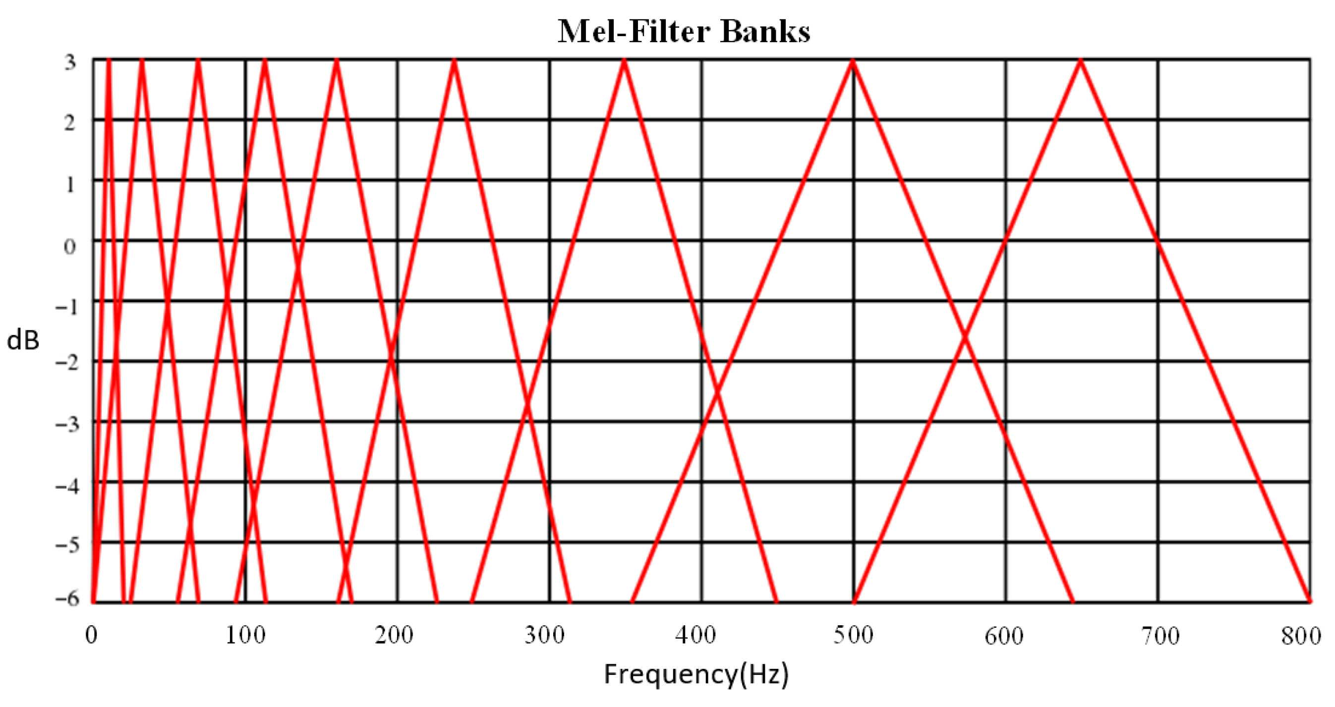
The Log-Mel spectrogram (Log-Mel) is a time–frequency analysis method inspired by the aural properties of the human ear. It overcomes the limitation of a uniform resolution in both the temporal and frequency domains by applying a series of Mel filter banks. The Mel frequency scale is nonlinear, as illustrated in Figure 6. These filters are arranged along the frequency axis from low to high frequency. In the low-frequency range, the filters are more numerous and densely distributed, resulting in narrower bandwidths and consequently a higher frequency resolution. This permits a crisper display of low-frequency spectrum components. By contrast, in the high-frequency range, the filters are fewer and more sparsely distributed, leading to wider bandwidths and thus improved temporal resolution.

According to the characteristics of ship-radiated noise, most of the acoustic energy is focused in the low-frequency region, which conveys richer and more informational components. Exploiting this feature enables for the greater detection of small details concealed in low-frequency areas of ship-radiated noise.

The mapping relationship between the acoustic frequency f and the Mel frequency $f_{mel}$ is given as

$$f_{mel}=2595{log}_{10}\left(1+{\displaystyle \frac{f}{700}}\right).$$

(7)

This nonlinear scale transforms the linear frequency axis into the Mel scale, as illustrated in Figure 7.

The process for extracting Log-Mel spectrogram features consists of the following steps:

(1) Preprocessing

Outlier removal, DC offset elimination, framing, and windowing are performed. A Hamming window is utilized for spectral smoothing.

(2) Discrete Fourier Transform (DFT)

The preprocessed signal is converted into the frequency domain as follows:

$$X_a\left(k\right)=\sum _{n=0}^{N-1}x\left(n\right)e^{-j2\pi /N},0\le k\le N$$

(8)

(3) Power Spectrum Calculation

The squared magnitude of the DFT provides the power spectrum as follows:

$$E(i,k)=|X_i{\left(k\right)|}^2$$

(9)

(4) Mel-Filtered Energies

The Mel filter bank comprises of M triangular band-pass filters. The center frequency of the m-th filter is computed as

$$f\left(m\right)={\displaystyle \frac{N}{F_s}}{B}^{-1}\left(B\left(f_l\left(m\right)\right)\right)+m{\displaystyle \frac{B\left(f_h\left(m\right)\right)-B\left(f_l\left(m\right)\right)}{M+1}},m=1,2,\dots ,M$$

(10)

where $f_l\left(m\right)$ and $f_h\left(m\right)$ denote the lower and upper boundaries of the filter, respectively, and $B\left(f\right)$ represents the Mel transformation. The transfer function of each triangular filter is given as

$$H_m\left(k\right)=\left\{\begin{array}{cc}0,\hfill & k<f(m-1)\hfill \\ {\displaystyle \frac{2(k-f(m-1\left)\right)}{\left(f\right(m+1)-f(m-1\left)\right)\left(f\right(m)-f(m-1\left)\right)}},\hfill & f(m-1)\le k\le f\left(m\right)\hfill \\ {\displaystyle \frac{2\left(f\right(m+1)-k)}{\left(f\right(m+1)-f(m-1\left)\right)\left(f\right(m+1)-f(m\left)\right)}},\hfill & f\left(m\right)\le k\le f(m+1)\hfill \\ 0,\hfill & k>f(m+1)\hfill \end{array}\right.$$

(11)

Based on the characteristics of ship-radiated noise, the number of filters is set at $M=128$, with frequency limits $f_l\left(m\right)=100$ Hz and $f_h\left(m\right)=1000$ Hz.

(5) Logarithmic Energy Compression

The filter bank energies are logarithmically compressed to reduce dynamic range as follows:

$$Log-mel\left(m\right)=ln\left(\sum _{k=0}^{N-1}E\left(k\right)H_m\left(k\right)\right)$$

(12)

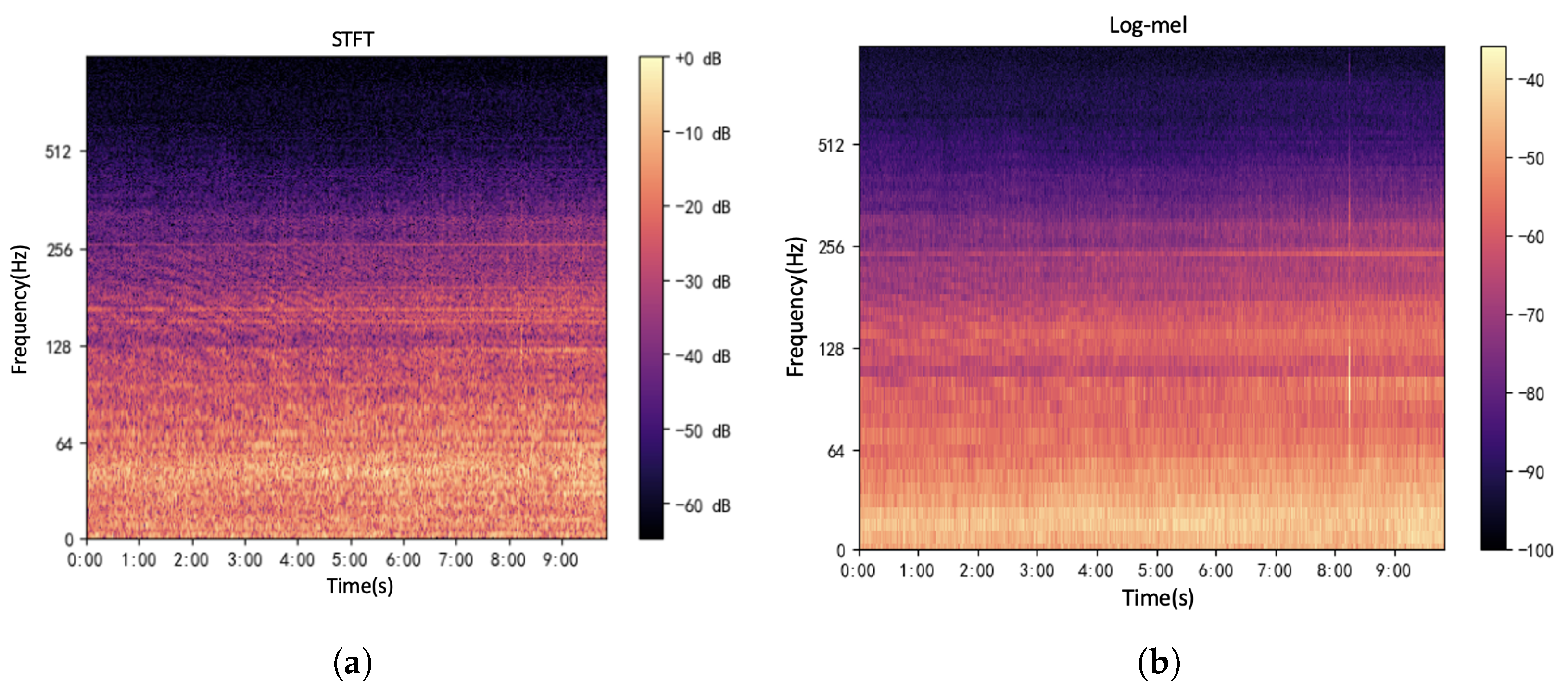
The Log-Mel spectrogram provides two key advantages: (a) it accentuates low-frequency components through perceptual scaling, (b) it reduces feature dimensionality, hence lowering computational complexity compared with STFT.

The STFT and Log-Mel spectrograms of ship-radiated noise are displayed in Figure 8.

3.1.2. Harmonic–Percussive Source Separation (HPSS)

Harmonic–Percussive Source Separation (HPSS) is a filtering-based technique designed to break down an acoustic signal into harmonic (H) and percussive (P) components. Harmonic sources are generally smooth and continuous along the time axis but exhibit discontinuities in frequency, whereas percussive sources demonstrate the opposite behavior: they are characterized by temporal discontinuities while remaining spectrally smooth, typically appearing as short-duration vertical broadband structures in the spectrogram [36].

This trait makes HPSS particularly ideal for evaluating ship-radiated noise, as it allows for the separation of line spectra (harmonic components) from broadband continuous spectra (percussive components). In passive underwater detection, this enables the separate examination of tonal and impulsive properties, hence boosting the interpretability of detection data. Moreover, because percussive signals usually correlate to transient interference, the application of HPSS efficiently suppresses impulsive noise, boosting signal clarity.

Consider a discrete input acoustic sound, where the harmonic signal $H_{h,i}$ and percussive signal $P_{h,i}$ are calculated by minimizing the following cost function:

$$J(H,P)={\displaystyle \frac{1}{2{\sigma }_H^2}}\sum _{h,i}{\left(H_{h,i-1}-H_{h,i}\right)}^2+{\displaystyle \frac{1}{2{\sigma }_P^2}}\sum _{h,i}{\left(P_{h,i-1}-P_{h,i}\right)}^2$$

(13)

subject to the constraint

$$H_{h,i}+P_{h,i}=X_{h,i},H_{h,i}>0, P_{h,i}>0$$

(14)

where ${\sigma }_H$ and ${\sigma }_P$ imply smoothing parameters for harmonic and percussive components, respectively. $H_{h,i}$ and $P_{h,i}$ represent the short-time Fourier transforms (STFTs) of the harmonic and percussive signals, while $X_{h,i}$ corresponds to the power spectrum of the input signal. The minimizing of $J(H,P)$ can be done by solving $\partial J/\partial H_{h,i}=0$ and $\partial J/\partial P_{h,i}=0$.

Based on mathematical principles, the following inequality can be applied:

$${(A-B)}^2\le 2{(A-C)}^2+2{(B-C)}^2$$

(15)

When $C=\left({\displaystyle \frac{A+B}{2}}\right)$, Equation (15) reduces to

$$2{(A-C)}^2+2{(B-C)}^2-{(A-C)}^2=4{\left(C-{\displaystyle \frac{A+B}{2}}\right)}^2$$

(16)

By substituting this result into the cost function, the following bounds for harmonic and percussive terms can be derived:

$${\left(H_{h,i-1}-H_{h,i}\right)}^2\le 2{\left(H_{h,i-1}-U_{h,i}\right)}^2+2{\left(H_{h,i}-U_{h,i}\right)}^2$$

(17)

$${\left(P_{h-1,i}-P_{h,i}\right)}^2\le 2{\left(P_{h-1,i}-V_{h,i}\right)}^2+2{\left(P_{h,i}-V_{h,i}\right)}^2$$

(18)

where $U_{h,i}=\left(H_{h,i-1}+H_{h,i}\right)/2$ and $V_{h,i}=\left(P_{h-1,i}+P_{h,i}\right)/2$. Introducing an auxiliary function Q, we have

$$\begin{array}{cc}\hfill Q(H,P,U,V)& ={\displaystyle \frac{1}{{\sigma }_H^2}}\sum _{h,i}\left\{{(H_{h,i-1}-U_{h,i})}^2+{(H_{h,i}-U_{h,i})}^2\right\}\hfill \\ \hfill & +{\displaystyle \frac{1}{{\sigma }_P^2}}\sum _{h,i}\left\{{(P_{h-1,i}-V_{h,i})}^2+{(P_{h,i}-V_{h,i})}^2\right\}\hfill \end{array}$$

(19)

which satisfies the following relation:

$$J(H,P)\le Q(H,P,U,V)$$

(20)

$$J(H,P)=\underset{U,V}{min}Q(H,P,U,V)$$

(21)

Using Equations (17)–(21), the following iterative updates can be derived:

$$\{U^{(k+1)},V^{(k+1)}\}=\underset{U,V}{min}Q\{H^{\left(k\right)},P^{\left(k\right)},U,V\}$$

(22)

$$\{H^{(k+1)},P^{(k+1)}\}=\underset{U,V}{min}Q\{H,P,U^{(k+1)},V^{(k+1)}\}$$

(23)

where k denotes the iteration index, $U_{h,i}$ and $V_{h,i}$ are auxiliary parameters, and Equations (22) and (23) assure that the cost function J declines monotonically. By iteratively applying these modifications, the harmonic and percussive components of ship-radiated noise can be efficiently removed.

This decomposition permits the more precise isolation of tone line spectra and broadband percussive characteristics in underwater acoustic data. Figure 9 presents an example, where panel (a) shows the original signal and panel (b) demonstrates the separated harmonic and percussive components using HPSS.

3.2. Detection Framework of CNN with Multi-Feature Inputs

3.2.1. Classification Evaluation Metrics

In binary classification tasks based on deep learning, accuracy is the most commonly used metric. When evaluating system performance with a validation set, each validation set is tested and the classification results are assessed using accuracy as the primary criterion. In addition, other metrics such as error rate, recall, and F1-score are also employed.

(1) Accuracy (ACC)

Accuracy refers to the proportion of accurately predicted samples to the total number of samples. It is defined as follows:

$$ACC={\displaystyle \frac{TP+TN}{TP+FP+FN+TN}}$$

(24)

where $TP$ means true positives, $TN$ denotes true negatives, $FP$ denotes false positives, and $FN$ denotes false negatives. The value of accuracy lies within the range $[0,1]$, and a bigger ACC indicates a better categorization ability.

(2) F1-score

The F1-score is a statistical metric used to evaluate the accuracy of a binary classification model. It is defined as the harmonic mean of precision P and recall R, providing a balanced measure that encompasses both false positives and false negatives. The F1-score varies between 0 and 1, where 1 denotes flawless categorization. The formula is given as

$$F1-score={\displaystyle \frac{2PR}{P+R}}={\displaystyle \frac{2\times TP}{2\times TP+FP+FN}}$$

(25)

(3) Confusion Matrix

The confusion matrix is a useful tool for testing binary classification models. It clearly indicates the fraction of successfully and wrongly identified samples for each class. The diagonal elements reflect valid predictions, whereas the off-diagonal elements represent misclassifications.

Table 5. Confusion matrix.

True Label	Predicted Label
	Signal	Noise
Signal	TP	FN
Noise	FP	TN

provides the $2\times 2$ confusion matrix used in this study.

3.2.2. Signal Detection Evaluation Metrics

(1) Receiver Operating Characteristic (ROC) curve

The ROC curve is a valuable tool for evaluating the detection ability of models, illustrating the trade-off between different types of mistakes under various task conditions. Consequently, it has been increasingly employed in the field of machine learning in recent years. As demonstrated in Figure 10, the horizontal axis of the ROC curve shows the false alarm rate (Pf), while the vertical axis reflects the true detection rate (Pd). Their definitions are presented as follows:

$$TPR={\displaystyle \frac{TP}{TP+FN}}$$

(26)

where $TPR$ corresponds to the detection probability in signal detection and the recall rate in deep learning.

$$FPR={\displaystyle \frac{FP}{FP+TN}}$$

(27)

where $FPR$ corresponds to the false alarm probability in signal detection.

By altering the decision threshold, samples with scores higher than the threshold are classed as positive, while those below the threshold are classified as negative. As the threshold decreases, more samples are categorized as positive, causing the number of true positives to increase, but also introducing more false positives. Therefore, both the TPR and FPR grow simultaneously. The closer the ROC curve approaches the upper-left corner $(0,1)$, the higher the detection performance.

(2) Area Under ROC Curve (AUC)

The area under ROC curve (AUC) is a metric generated from the ROC curve, as depicted in Figure 10. AUC is the area under the ROC curve. When ROC curves meet, it becomes impossible to directly demonstrate superiority through simple comparison; therefore the idea of AUC gives a more straightforward measure of performance. The value of AUC varies from 0.5 to 1, where a bigger AUC indicates a better detection performance. In the ideal condition, the AUC value hits 1.

In this study, accuracy, F1-score, confusion matrix, ROC, and AUC are used as the evaluation measures for the CNN detector.

3.3. Design and Construction of Convolutional Neural Network Models

3.3.1. Model Construction

In this study, the network structures were designed with reference to the literature, and combined with the characteristics of ship-radiated noise. Three types of CNN architectures with 6, 10, and 14 layers were constructed, as shown in

Table 6. CNN architectures with different layers.

CNN6	CNN10	CNN14
STFT
(5 × 5 @ 64, BN, ReLU)	(3 × 3 @ 64, BN, ReLU) × 2	(3 × 3 @ 64, BN, ReLU) × 2
2 × 2 Max Pooling
(5 × 5 @ 128, BN, ReLU)	(3 × 3 @ 128, BN, ReLU) × 2	(3 × 3 @ 128, BN, ReLU) × 2
2 × 2 Max Pooling
(5 × 5 @ 256, BN, ReLU)	(3 × 3 @ 256, BN, ReLU) × 2	(3 × 3 @ 256, BN, ReLU) × 2
2 × 2 Max Pooling
(5 × 5 @ 512, BN, ReLU)	(3 × 3 @ 512, BN, ReLU) × 2	(3 × 3 @ 512, BN, ReLU) × 2
Fully Connected 32	Fully Connected 32	2 × 2 Max Pooling
Fully Connected 2	Fully Connected 2	(3 × 3 @ 1024, BN, ReLU) × 2
		2 × 2 Max Pooling
		(3 × 3 @ 2048, BN, ReLU) × 2
		Fully Connected 32
		Fully Connected 2

.

STFT was adopted as the time–frequency input characteristic for the networks. The batch size was set to 16, with the number of training epochs $EPOCH=60$ and learning rate $lr=0.001$.

Table 7. Comparison of training accuracy among different network models.

Network Structure	6-Layer CNN	10-Layer CNN	14-Layer CNN
ACC	93.609%	95.407%	94.204%

provides the optimal classification accuracy results of different CNN architectures under the same input features. Based on a comparison of the results, the 10-layer Convolutional Neural Network (CNN) was ultimately selected as the network model for this experiment.

3.3.2. Parameter Selection

The main parameters of the network model are as follows.

(1) Batch size

Batch size refers to the number of training samples selected from the dataset for each iteration. One iteration refers to training once with a batch of samples, while one epoch corresponds to training once with the complete dataset. The batch size directly influences the degree and speed of model improvement, as well as GPU memory utilization. In order to explore the influence of batch size on the developed CNN detector, a batch size of 16 was selected in this work. The detailed network model parameters are shown in

Table 8. Network model parameters.

Name	Parameter Value
Convolution Stride	2
Convolution Kernel Size	$3\times 3$
Activation Function	ReLU
Optimizer	SGD
Loss Function	BCELoss
Pooling Layer	Max Pooling
Pooling Size	$2\times 2$
Pooling Stride	2
Learning Rate	Variable learning rate [0.001, 0.0001]; fixed learning rate [0.001, 0.0001]
Batch Size	8, 16, 32

.

(2) Learning rate (LR)

The learning rate is one of the most critical hyperparameters in a convolutional neural network, as it dictates whether the objective function can converge to a local minimum and how soon convergence happens. If the learning rate is too big, the optimization may overshoot the optimum; on the other hand, if it is too little, optimization efficiency may be low and convergence may not be attained within an acceptable time. Therefore, the learning rate plays a key role in the performance of the algorithm. In addition to adopting a set learning rate, several adaptive techniques are often applied in network training, which may be fixed or changeable. The learning rate is defined as

$$lr=dro{p}^{EPOCH}·l{r}_0$$

(28)

where $l{r}_0$ signifies the starting learning rate, $EPOCH$ is the training epoch, and $drop$ is the decay factor, fixed to $0.9$ in this case. Thus, $lr$ reflects the learning rate at each training period. The learning rate corresponding to different epochs are depicted in Figure 11.

3.4. Parameter Impact Analyses on Network Training

The hardware environments used here are shown in

Table 9. Hardware environment.

Name	Parameter Value
Processor	Intel Xeon Silver 4180
Memory	12 GB
GPU	GeForce RTX 2080Ti

. Based on this configuration of the computational environment, this subsection mainly analyzed the influence of batch size and learning rate selection.

3.4.1. Impact of Batch Size on Network Training

The loss curves of the network model during training when STFT is selected as the feature extraction method, with $EPOCH=60$ and a fixed learning rate of $lr=0.0001$. The curves illustrate, as presented in Figure 12, that the training loss fluctuates with the number of iterations under different batch sizes. The horizontal axis shows the number of iterations, whereas the vertical axis represents the training loss. The black, red, and green curves correspond to batch sizes of 8, 16, and 32, respectively, from smaller to larger.

It can be noted that as the number of iterations grows, the training loss gradually lowers and begins to stabilize. When the batch size is smaller, the training loss exhibits bigger oscillations. In contrast, with higher batch sizes, the training loss drops more rapidly, and the network converges faster, hence speeding up the processing speed for the same amount of input.

Table 10. Training time of models with different batch sizes.

Batch Size	Time per Iteration (s)	Iterations per EPOCH	Training Time (min)
8	0.05	8178	272.6
16	0.11	4089	299.9
32	0.20	2045	409.0

presents the impact of different batch sizes on the training time when STFT was selected as the feature extraction method, with $EPOCH=60$ and $lr=0.0001$. It can be observed that as the batch size increases, the time per iteration becomes longer, while the number of iterations per epoch decreases, resulting in a shorter total training time.

3.4.2. Impact of Learning Rate on Network Training

The training loss curves of the network model are analyzed with the Log-Mel input feature and the batch size is fixed to 16. The curves are shown in Figure 13, where the training loss changes with the number of iterations under different learning rate settings. The red curve represents a fixed learning rate of $lr=0.001$, the green curve represents a fixed learning rate of $lr=0.0001$, the black curve represents a variable learning rate with an initial $lr=0.001$, and the blue curve represents a variable learning rate with an initial $lr=0.0001$.

It can be observed that with larger learning rates, the loss function decreases more rapidly and the network converges faster. Moreover, the variable learning rate achieves faster convergence compared with the fixed learning rate.

3.5. Performance Comparison of Different Input Time–Frequency Features

In this section, an analysis was carried out on different input time–frequency features, including STFT, Log-Mel, HPSS (H), and Log-Mel+HPSS (H). The 10-layer Convolutional Neural Network (CNN) was used as the training model. The convolution kernels in the convolutional layers were set to a size of $3\times 3$ with a stride of 2. For the pooling layers, the pooling size was $2\times 2$, and the pooling method was max pooling. The fully linked layers had 32 and 2 neurons. The loss function was the binary cross-entropy loss method, and the optimization algorithm was Stochastic Gradient Descent (SGD). The number of training epochs was set to $EPOCH=60$. For each feature, a total of 12 tests were performed with a batch size of 16 and a fixed learning rate of 0.0001, resulting in 60 experiments across the four features. During training, the validation accuracy at each epoch was recorded, and at the end of each experiment, the best validation accuracy and the associated epoch were reported.

3.5.1. Comparison of Input Dimensions

In this experiment, one-dimensional acoustic data are transformed into two-dimensional matrices by multiple feature transformations, which are then used as inputs to the neural network for training and testing.

Table 11. Input dimensions of different features.

Time–Frequency Feature	Input Dimension
STFT	513 × 77
Log-Mel	128 × 77
HPSS(H)	128 × 77
Log-Mel + HPSS(H)	128 × 77

provides the input dimensions corresponding to each feature type.

3.5.2. Comparison of Training Time

Table 12. Comparison of network training time for different time–frequency features.

Time–Frequency Feature	Time per Iteration (s)	Training Time (min)
STFT	0.11	299.9
Log-Mel	0.03	81.76
H	0.028	76.3
Log-Mel + HPSS(H)	0.033	89.9

compares the training times of the CNN under different input features, with the batch size set at 16, training length of 60 epochs, learning rate of 0.0001, and 4089 iterations per epoch.

From Table 12, it can be noted that with the same batch size, the training time per iteration for STFT is much longer. The training times for Log-Mel, H, and Log-Mel + HPSS(H) features are about the same. It may be extrapolated from Table 12 that for the STFT feature, due to the huge input dimension of the network, additional parameters are required. As a result, each cycle of training using STFT takes approximately three times longer than with the other features. This means that STFT consumes more memory and has inferior computing efficiency.

3.5.3. Comparison of Training and Test Results

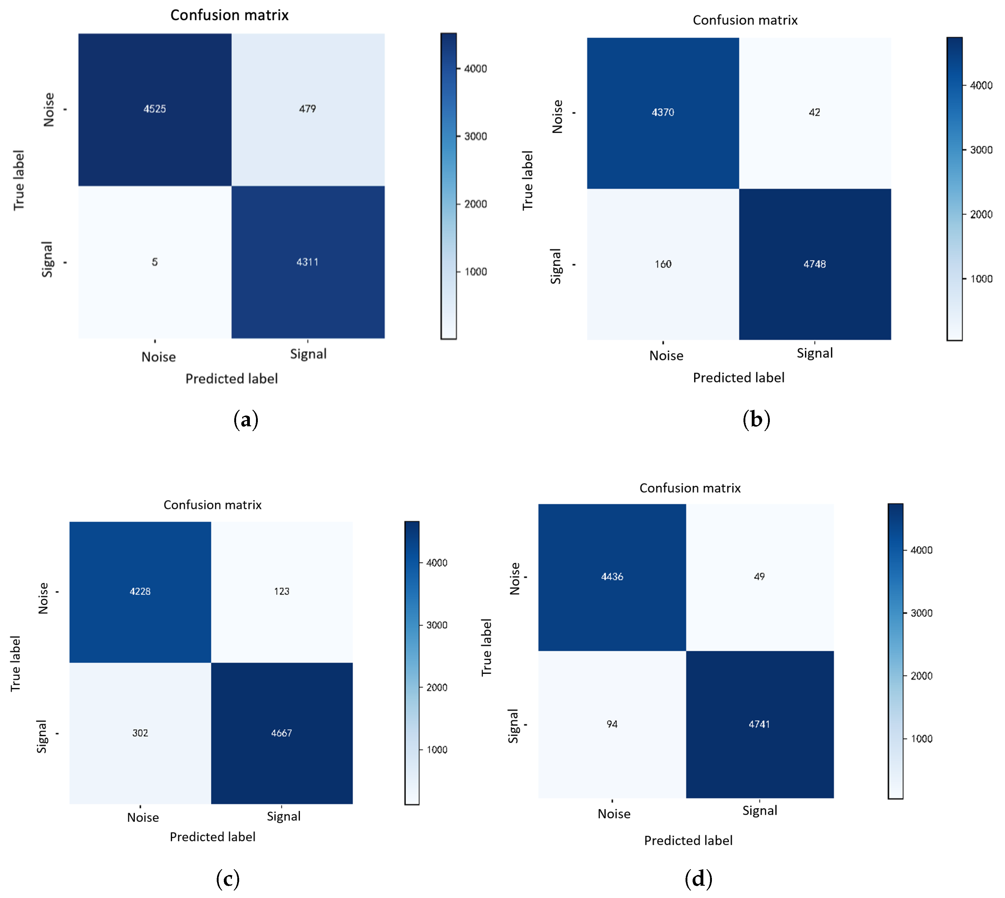
Figure 14a–d illustrate the confusion matrix findings of the optimal models for different characteristics on the test set. It can be shown that all four types of characteristics are able to efficiently distinguish between ship-radiated noise and ocean background noise in the context of binary classification.

Figure 15 shows a comparison of the F1-score results for the four different input features. The x-axis represents the features, while the y-axis indicates the corresponding F1-score.

From Figure 15, it can be shown that, under the identical test dataset, Log-Mel + HPSS(H) obtains the best detection performance, followed by HPSS(H), Log-Mel, and STFT. Through a comparison between Log-Mel and STFT, we can observe a roughly 0.25% improvement. Since ship-radiated noise is predominantly concentrated in the low-frequency band region, the Log-Mel feature can disclose more detailed aspects of low-frequency sound signals. HPSS(H) can produce a 3.06% improvement compared with STFT, which is superior. In the examination of non-Gaussian and impulsive ocean noise, the use of HPSS can perform better with impulsive noise interference removal. By applying Log-Mel and HPSS(H) features at the same time, the detailed features of low frequencies are highlighted in accordance with impulsive noise interferences removal, and hence, show the best performance.

3.5.4. Comparison of Detection Performance

For binary hypothesis testing in this study, there are two hypotheses: one indicating that the received data contains ship-radiated noise, and the other indicating that the received data contains ocean background noise.

$$H_1:x\left(t\right)=s\left(t\right)+n\left(t\right)$$

(29)

$$H_0:x\left(t\right)=n\left(t\right)$$

(30)

The continuous cruise experiment dataset is $I=\{x_1,x_2,\dots ,x_j\}$, which is fed into a designed convolutional neural network (CNN) detector. The CNN detector outputs two results: $M=\left\{\left(P_{s_k},P_k=1\right),\left(P_{n_k},P_k=0\right)\mid k=1,2,\dots ,J\right\},$ corresponding to the probability of being classified as a target ($P_{s_k}$) and the probability of being classified as noise ($P_{n_k}$), with $P_{n_k}+P_{s_k}=1$. The positive sample probability is used as the test statistic: $T\left(x\right)=\left\{\left(P_{s_k},P_k=1\right)\mid k=1,2,\dots ,J\right\}.$ When the noise dataset is input into the same CNN detector, two results are also obtained: $N=\left\{\left(P_{s_k},P_k=1\right),\left(P_{n_k},P_k=0\right)\mid k=1,2,\dots ,J\right\}.$ The probability of being classified as a target is extracted as $N_0=\left\{\left(S_k,P_k=1\right)\mid k=1,2,\dots ,K\right\},$ and the results are sorted in descending order. Under the Neyman–Pearson criterion, given the false alarm probability $P_f$, the detection threshold $\gamma$ is calculated as follows:

$$\gamma =N_0\left(1-P_f\right)K$$

(31)

The decision rule for signal detection is given by

$$T\left(x\right)\underset{H_0}{\overset{H_1}{\gtrless }}\gamma$$

(32)

The detection probability calculation process for continuous on-the-fly experimental data is shown in the table below.

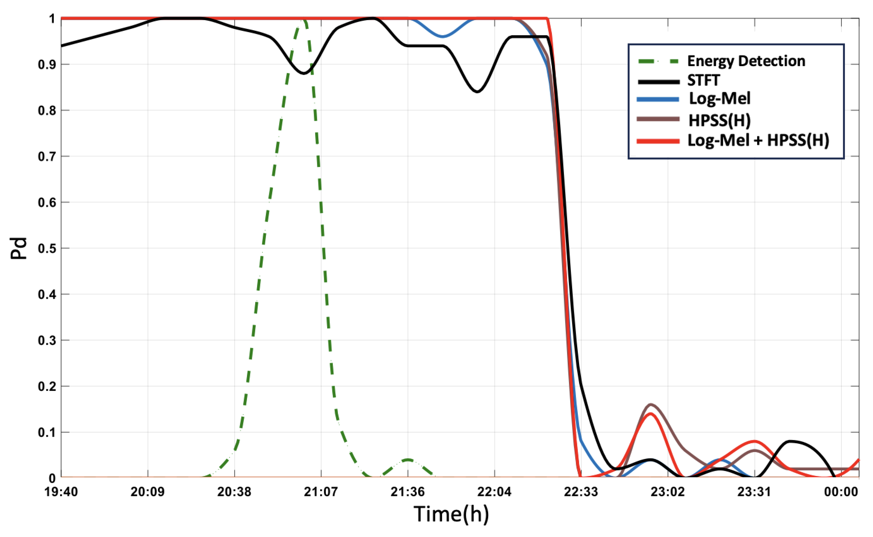
Following the procedure described in

Table 13. Detection probability calculation process for continuous navigation experimental data.

Detection Probability Calculation Process
Step 1	Send the noise dataset into the designed CNN detector to obtain the probability of being judged as a target: $N_0=\{(S_k,P_k=1)\mid k=1,2,\dots ,K\}$.
Step 2	Sort $\left\{S_k\right\},\forall k:S_k\in N_0$ in descending order.
Step 3	Set the false alarm probability $P_f$ and determine the threshold $\gamma =N_0(1-P_f)K$.
Step 4	Send the real experimental data into the CNN detector to obtain the probability of being judged as a target: $T\left(x\right)=\{(P_{s_k},P_k=1)\mid k=1,2,\dots ,J\}$.
Step 5	Divide $N_1$ into groups with $M=50$ samples per group to obtain Q groups. Count, in each group, the number of times exceeding the threshold $\gamma$, denoted by $M_y$. Finally, the detection probability for the continuous navigation experimental data is $P_i=M_{\gamma }/M,i=1,2,\dots ,Q$.

, detection curves for different features were computed based on the continuous navigation data and compared with the conventional energy detection method.

Figure 16 illustrates the ROC curves for the test set for different features. The curves in dark blue, black, red, and magenta correspond to the STFT, Log-Mel, HPSS(H), and Log-Mel + HPSS(H) features, respectively, while the light blue curve represents the broadband energy detection baseline. As expected, the detection probability increases with the false alarm probability. Compared with classical energy detection, all four feature-based approaches demonstrate a considerably superior performance. Among these, STFT provides the lowest AUC, whereas Log-Mel + HPSS(H) achieves the highest AUC, suggesting the strongest generalization capacity and best overall detection performance. This finding is congruent with the conclusions drawn from the F1-score comparison.

Table 14. Comparison of detection performance across different features.

Time–Frequency Features	Batch Size	Learning Rate	Best EPOCH	F1-Score	AUC	Validation ACC
STFT	16	Variable 0.001	12	0.94920	0.97800	0.95708
Log-Mel	16	Variable 0.001	17	0.95210	0.98500	0.96000
HPSS(H)	16	Variable 0.001	21	0.97830	0.99200	0.97952
Log-Mel + HPSS(H)	16	Variable 0.001	33	0.98400	0.99800	0.98732

summarizes the best validation accuracy obtained for each feature with its corresponding optimal batch size and learning rate. To further evaluate the generalization ability, the models were tested on the test dataset, yielding the AUC and F1-score results. It can be seen that, under the same CNN model, the optimal hyperparameters (batch size and learning rate) vary depending on the feature dimension and intrinsic properties of the feature.

4. Experimental Verification

4.1. Experiment Description

To evaluate the efficiency of the proposed approaches in practice, a set of sea experiment data is adopted, which was collected in the South China Sea. A deep sea latent buoy is deployed at 1700 m depth. The design of the experimental ship’s navigation survey line is depicted in Figure 17a,b. The ship started at point A, and sailed down the red dashed line to points B, C, and finished at $X_1$. The distance of the buoy from point A to point B is approximately 10 km, while point C is approximately 56 km away. As illustrated in Figure 18, from 20:00 to 24:00, a total of 4 h of received ship-radiated signals are evaluated with LOFAR. In view of the temporal frequency data, the line spectral signatures of the experimental ship may be seen at a short distance, although they are fully drowned out by ocean ambient noise.

4.2. Detection Performance Analysis

Following the above method, detection curves for different features were computed using the continuous navigation experiment data and compared with the traditional energy detection method. The graphic illustrates the curves after applying curve fitting to the results.

As demonstrated in Figure 19, the performance comparison of different input characteristics (STFT, Log-Mel, HPSS(H), and Log-Mel + HPSS(H)) at a false alarm probability $P_f=0.01$ is presented, as well as the standard energy detection approach. It can be observed that, for the same false alarm probability, the detection performance of all CNN-based features (STFT, Log-Mel, HPSS(H), Log-Mel + HPSS(H)) is much more superior than that of the classic energy detection approach. For ship-radiated noise within 10 km, all four characteristics’ trained networks can reliably detect the target. Among these, Log-Mel + HPSS(H) achieves the best overall performance, suggesting that complementary information increases detection capabilities. Log-Mel alone likewise performs strongly, while HPSS(H) as a solo input feature displays a somewhat lower performance, further demonstrating its limited representational ability when employed in isolation.

Figure 20 further presents the detection results of the Log-Mel + HPSS(H) feature compared with traditional energy detection at different false alarm probabilities ($P_f=0.01,P_f=0.05,P_f=0.1$), which can further demonstrate its superior detection performance compared with the traditional energy detection method.

5. Discussions

Based on the methodological developments and experimental outcomes, the following discussions are highlighted.

(1) The building of a specific dataset for passive underwater target identification, suited to the peculiarities of ship transit, represents a foundational contribution of this work. The eight-day field experiment provided a realistic acoustic environment with ship-radiated noise, ambient noise, and the interference of the deep sea very-low-frequency band. The pre-processing and labeling methodology established a clear norm for data preparation in this domain. Additionally, the application of data augmentation techniques solved the key issue of class imbalance, which is a prevalent challenge in real-world underwater acoustic datasets. Most notably, the novel incorporation of Log-mel and HPSS characteristics, adopted from speech recognition, for characterizing ship-radiated noise has been highly effective. This cross-domain feature transfer highlights the possibility of employing advanced audio processing techniques in underwater acoustics, with the exact extraction parameters supplied affording useful guidance for future research.

(2) The suggested CNN-based detection framework has proved both its feasibility and superiority over standard energy detection approaches. The carefully developed 10-layer CNN architecture, tailored for ship-radiated noise characteristics, coupled with appropriate assessment metrics bridging deep learning and signal detection theory, creates a comprehensive detection technique. The comprehensive analysis of diverse network parameters provides vital insights into model optimization. The comparative analysis of time–frequency features demonstrates that Log-mel features obtained an optimal performance by efficiently capturing the low-frequency properties of ship noise while maintaining computing economy. This achievement underlines the importance of feature design that matches with both the physical features of the target signals and practical implementation constraints.

However, several issues and future directions demand attention:

(1) The complexity and variety of ship-radiated noise need more robust feature representations. While the current features show promising results, future work should focus on using deep learning’s powerful representation learning capabilities to construct more sophisticated feature fusion algorithms. This could involve researching attention mechanisms or multi-modal learning methodologies that can better manage complicated maritime environments and improve the system’s generalization potential.

(2) The data imbalance problem remains a key worry. Although data augmentation techniques were applied in this study, more advanced alternatives such as generative adversarial networks (GANs) for synthetic data generation, or cost-sensitive learning approaches deserve additional consideration. As deep learning models are essentially data-driven, creating more complex data handling solutions will be crucial for progressing this field of study.

(3) Future work will also focus on constructing more efficient network topologies and researching semi-supervised learning approaches to lessen the dependency on huge labeled datasets, ultimately moving toward more practical and deployable underwater target detection systems.

6. Conclusions

This paper proposed a hybrid Log-Mel and HPSS feature-aided deep CNN detection framework for underwater very-low-frequency remote passive sonar detection. A systematic non-Gaussian statistical study of deep sea VLF ocean noise is offered with a week-long noise dataset. On the basis of this, a hybrid Log-Mel and HPSS feature-aided deep CNN detection framework is built, aiming to emphasize the detailed characteristics of low frequencies in accordance with impulsive noise interference removal. A 10-layer optimum CNN was trained and tested with hybrid Log-Mel and HPSS features, and the detection is compared with traditional STFT, Log-Mel, and HPSS. The performance is further verified using a set of deep sea experiment data in the South China Sea, which may indicate its superior performance. From the application perspective, the advantages of the suggested method have proven the highly superior detection ability to overcome low SNR and low false alarm rate problem, especially under complicated non-Gaussian and impulsive background noise. In view of this, this work can make a beneficial contribution to resolving the issues of underwater extremely low-frequency remote passive sonar detection, and can provide an important and efficient paradigm for intelligent passive sonar detection. For future work, we will focus on developing more efficient network architectures and exploring semi-supervised learning approaches to reduce the dependency on large labeled datasets, ultimately moving toward more practical and deployable underwater target detection systems.

References

1. Etter, P.C. Advanced applications for underwater acoustic modeling. Adv. Acoust. Vib. 2012, 2012, 214839. [Google Scholar] [CrossRef]
2. Dong, H.; Wang, H.; Shen, X.; He, K. Parameter matched stochastic resonance with damping for passive sonar detection. J. Sound Vib. 2019, 458, 479–496. [Google Scholar] [CrossRef]
3. Bossér, D.; Hendeby, G.; Nordenvaad, M.L.; Skog, I. Broadband passive sonar track-before-detect using raw acoustic data. IEEE J. Ocean. Eng. 2025. [Google Scholar] [CrossRef]
4. Ross, D. Mechanics of Underwater Noise; Pergamon Press: New York, NY, USA, 1976; pp. 272–280. [Google Scholar]
5. Urick, R.J. Principles of Underwater Sound; McGraw-Hill: New York, NY, USA, 1983; pp. 266–284. [Google Scholar]
6. Arveson, P.T.; Vendittis, D.J. Radiated noise characteristics of a modern cargo ship. J. Acoust. Soc. Am. 2000, 107, 118–129. [Google Scholar] [CrossRef] [PubMed]
7. Wang, Z.; Guo, J.; Zhang, S.; Xu, N. Marine object detection in forward-looking sonar images via semantic-spatial feature enhancement. Front. Mar. Sci. 2025, 12, 1539210. [Google Scholar] [CrossRef]
8. Nikias, C.L.; Shao, M. Signal Processing with Alpha-Stable Distributions and Applications; Wiley-Interscience: New York, NY, USA, 1995. [Google Scholar]
9. Andrew, R.K.; Howe, B.M.; Mercer, J.A.; Dzieciuch, M.A. Ocean ambient sound: Comparing the 1960s with the 1990s for a receiver off the California coast. Acoust. Res. Lett. Online 2002, 3, 65–70. [Google Scholar] [CrossRef]
10. Wang, J.; Li, J.; Yan, S.; Shi, W.; Yang, X.; Guo, Y.; Gulliver, T.A. A novel underwater acoustic signal denoising algorithm for Gaussian/non-Gaussian impulsive noise. IEEE Trans. Veh. Technol. 2020, 70, 429–445. [Google Scholar] [CrossRef]
11. Haining, H.; Yu, L. Underwater acoustic detection: Current status and future trends. Bull. Chin. Acad. Sci. (Chin. Version) 2019, 34, 264–271. [Google Scholar]
12. Roch, M.A.; Soldevilla, M.S.; Burtenshaw, J.C.; Henderson, E.E.; Hildebrand, J.A. Gaussian mixture model classification of odontocetes in the Southern California Bight and the Gulf of California. J. Acoust. Soc. Am. 2007, 121, 1737–1748. [Google Scholar] [CrossRef]
13. Bertilone, D.C.; Killeen, D.S. Statistics of biological noise and performance of generalized energy detectors for passive detection. IEEE J. Ocean. Eng. 2001, 26, 285–294. [Google Scholar] [CrossRef]
14. Mahmood, A.; Chitre, M. Modeling colored impulsive noise by Markov chains and alpha-stable processes. In Proceedings of the OCEANS 2015—Genova, Genova, Italy, 18–21 May 2015; IEEE: Piscataway, NJ, USA, 2015; pp. 1–7. [Google Scholar]
15. Pieniazek, R.; Beach, R.; Dycha, G.; Mickle, M.; Higgs, D. Navigating noisy waters: A review of field studies examining anthropogenic noise effects on wild fish. J. Acoust. Soc. Am. 2023, 154, 2828–2842. [Google Scholar] [CrossRef]
16. Yang, J.; Nystuen, J.A.; Riser, S.C.; Thorsos, E.I. Open ocean ambient noise data in the frequency band of 100 Hz–50 kHz from the Pacific Ocean. JASA Express Lett. 2023, 3, 036001. [Google Scholar] [CrossRef]
17. Mo, X.; Wen, H.; Yang, Y.; Zhou, H.; Ruan, H. Statistical characteristics of under-ice noise on the Arctic Chukchi Plateau. J. Acoust. Soc. Am. 2023, 154, 2489–2498. [Google Scholar] [CrossRef]
18. Ritu, J.; Van Dine, A.; Peeples, J. Quantitative Measures for Passive Sonar Texture Analysis. arXiv 2025, arXiv:2504.14843. [Google Scholar] [CrossRef]
19. Weinberg, G.V.; van der Merwe, M. Passive Sonar Sensor Placement for Undersea Surveillance. arXiv 2025, arXiv:2503.03940. [Google Scholar] [CrossRef]
20. Kassam, S.A. Signal Detection in Non-Gaussian Noise; Springer Science & Business Media: New York, NY, USA, 2012. [Google Scholar]
21. Hongwei, Z.; Wang, H.; Yongsheng, Y.; Haiyang, Y.; Haitao, D. Remote passive sonar detection by relative multiscale change entropy. IEEE Sens. J. 2022, 22, 18066–18075. [Google Scholar] [CrossRef]
22. Dong, H.; Shen, X.; He, K.; Wang, H. Nonlinear filtering effects of intrawell matched stochastic resonance with barrier constrainted duffing system for ship radiated line signature extraction. Chaos Solitons Fractals 2020, 141, 110428. [Google Scholar] [CrossRef]
23. Dong, H.; Ma, S.; Suo, J.; Zhu, Z. Matched stochastic resonance enhanced underwater passive sonar detection under non-Gaussian impulsive background noise. Sensors 2024, 24, 2943. [Google Scholar] [CrossRef]
24. Yao, H.; Gao, T.; Wang, Y.; Wang, H.; Chen, X. Mobile_ViT: Underwater acoustic target Recognition Method based on local–global feature fusion. J. Mar. Sci. Eng. 2024, 12, 589. [Google Scholar] [CrossRef]
25. Tang, J.; Gao, W.; Ma, E.; Sun, X.; Ma, J. Deep Learning Based Underwater Acoustic Target Recognition: Introduce a Recent Temporal 2D Modeling Method. Sensors 2024, 24, 1633. [Google Scholar] [CrossRef] [PubMed]
26. Suo, J.; Wang, H.; Yan, Y.; Shen, X. Deep stochastic resonance array and its application in enhancing underwater weak signals. Nonlinear Dyn. 2025, 113, 5193–5214. [Google Scholar] [CrossRef]
27. Bogdan, F.; Lascu, M.R. Advances and Challenges in Deep Learning for Acoustic Pathology Detection: A Review. Technologies 2025, 13, 329. [Google Scholar] [CrossRef]
28. Xu, W.; Han, X.; Zhao, Y.; Wang, L.; Jia, C.; Feng, S.; Han, J.; Zhang, L. Research on Underwater Acoustic Target Recognition Based on a 3D Fusion Feature Joint Neural Network. J. Mar. Sci. Eng. 2024, 12, 2063. [Google Scholar] [CrossRef]
29. Ji, F.; Ni, J.; Li, G.; Liu, L.; Wang, Y. Underwater acoustic target recognition based on deep residual attention convolutional neural network. J. Mar. Sci. Eng. 2023, 11, 1626. [Google Scholar] [CrossRef]
30. Aslam, M.A.; Zhang, L.; Liu, X.; Irfan, M.; Xu, Y.; Li, N.; Zhang, P.; Jiangbin, Z.; Yaan, L. Underwater sound classification using learning based methods: A review. Expert Syst. Appl. 2024, 255, 124498. [Google Scholar] [CrossRef]
31. Zali, Z.; Rein, T.; Krüger, F.; Ohrnberger, M.; Scherbaum, F. Ocean bottom seismometer (OBS) noise reduction from horizontal and vertical components using harmonic–percussive separation algorithms. Solid Earth 2023, 14, 181–195. [Google Scholar] [CrossRef]
32. González-Martínez, F.; Carabias-Orti, J.; Cañadas-Quesada, F.; Ruiz-Reyes, N.; Martínez-Muñoz, D.; García-Galán, S. Improving snore detection under limited dataset through harmonic/percussive source separation and convolutional neural networks. Appl. Acoust. 2024, 216, 109811. [Google Scholar] [CrossRef]
33. Xie, Y.; Ren, J.; Xu, J. Adaptive ship-radiated noise recognition with learnable fine-grained wavelet transform. Ocean. Eng. 2022, 265, 112626. [Google Scholar] [CrossRef]
34. Kek, X.Y.; Chin, C.S.; Li, Y. Acoustic scene classification using bilinear pooling on time-liked and frequency-liked convolution neural network. In Proceedings of the 2019 IEEE Symposium Series on Computational Intelligence (SSCI), Xiamen, China, 6–9 December 2019; IEEE: Piscataway, NJ, USA, 2019; pp. 3189–3194. [Google Scholar]
35. He, Q.; Wang, H.; Zeng, X.; Jin, A. Ship-Radiated Noise Separation in Underwater Acoustic Environments Using a Deep Time-Domain Network. J. Mar. Sci. Eng. 2024, 12, 885. [Google Scholar] [CrossRef]
36. Podder, P.; Khan, T.Z.; Khan, M.H.; Rahman, M.M. Comparative performance analysis of hamming, hanning and blackman window. Int. J. Comput. Appl. 2014, 96, 1–7. [Google Scholar] [CrossRef]
Figure 1. Ship navigation route map.
Jmse 13 02030 g001
Figure 2. Time–frequency plots of ship-radiated noise and ocean environmental noise: (a) ship-radiated noise, (b) ocean environmental noise.
Jmse 13 02030 g002
Figure 3. Time–frequency map of typical ocean ambient noise measured in the South China Sea (50 min).
Jmse 13 02030 g003
Figure 4. Estimation of characteristic exponent ( S α S ) of measured very-low-frequency ocean ambient noise.
Jmse 13 02030 g004
Figure 5. (a) Kurtosis distribution of measured noise segments above 100 Hz. (b) Kurtosis distribution of measured noise segments below 100 Hz.
Jmse 13 02030 g005
Figure 6. Mel filter bank.
Jmse 13 02030 g006
Figure 7. The mapping relationship between frequency f and Mel frequency f m e l .
Jmse 13 02030 g007
Figure 8. (a) STFT spectrogram. (b) Log-Mel spectrogram.
Jmse 13 02030 g008
Figure 9. Original signal and HPSS: (a) original signal. (b) HPSS.
Jmse 13 02030 g009
Figure 10. An illustrative ROC curve and AUC.
Jmse 13 02030 g010
Figure 11. Variation of the learning rate with different EPOCH values.
Jmse 13 02030 g011
Figure 12. Comparison of training loss across different batch sizes.
Jmse 13 02030 g012
Figure 13. Training loss with different learning rates.
Jmse 13 02030 g013
Figure 14. Confusion matrix results for different features: (a) STFT, (b) Log-Mel, (c) HPSS(H), (d) Log-Mel + HPSS(H).
Jmse 13 02030 g014
Figure 15. Comparison of F1-score results for different features.
Jmse 13 02030 g015
Figure 16. ROC curves for different time–frequency features with CNN.
Jmse 13 02030 g016
Figure 17. (a) Schematic diagram of target perception test for submerged targets. (b) Ocean survey line.
Jmse 13 02030 g017
Figure 18. Time–frequency plot of navigation from 20:00 on 16 May to 00:00 on 17 May.
Jmse 13 02030 g018
Figure 19. Detection probability curves for different features at P f = 0.01 .
Jmse 13 02030 g019
Figure 20. Comparison of Log-Mel feature and energy detection performance at different false alarm probabilities.
Jmse 13 02030 g020