Identification Modeling of Ship Maneuvering Motion Based on AE-MSVR

Abstract

The strong coupling between the ship’s sway and yaw motion increases the complexity of identifying hydrodynamic derivatives in mathematical models and reduces accuracy. To solve this problem, this paper proposes an identification method Alpha Evolution Multi-output Support Vector Regression (AE-MSVR) based on MSVR combined with AE. This method approaches the yaw and sway motion equations as a multi-input and multi-output (MIMO) problem, utilizing MSVR for modeling and optimizing hyperparameters with AE. It reduces parameter drift by restructuring the regression model’s input–output. Identification data is obtained via zigzag test simulation. The AE-MSVR method successfully identifies linear and nonlinear hydrodynamic derivatives in the 3 degree of freedom (DOF) Abkowitz model. Using clean simulation data, the results show promising agreement with experimental values from planar motion mechanism (PMM) tests and achieve improved accuracy compared with the standard SVR identification method. To assess robustness, simulated noise is introduced at different levels; maneuvering characteristics are evaluated using turning circle tests. Results demonstrate that AE-MSVR achieves promising accuracy in identifying ship hydrodynamic derivatives and shows encouraging robustness against noise. The method provides potential support for ship motion prediction and maneuverability forecasting.

1. Introduction

The trend toward larger and more specialized vessels has significantly increased maneuvering difficulties and accident risks, making the prediction of ship maneuverability crucial for navigation safety. The International Maritime Organization (IMO) issued the interim guidelines on the second generation intact stability criteria in 2020, imposing higher requirements on maneuverability analysis [1]. Predicting maneuverability primarily relies on simulation using mathematical models [2]. Although accurate models are crucial for effective prediction, identifying the necessary hydrodynamic derivatives remains challenging, particularly for the yaw and sway equations due to their strong coupling. Developing efficient and accurate hydrodynamic derivatives identification methods has important theoretical value and application prospects.

Establishing a mathematical model for ship maneuvering motion primarily involves determining its structure and parameters. Common hydrodynamic models include the whole model named by Professor Abkowitz [3] and the MMG model proposed by the Japanese Mathematical Modeling Group. Regardless of the type of mathematical model employed, accurately obtaining hydrodynamic derivatives within the model is crucial for enhancing the precision of ship motion prediction. System identification (SI) theory provides an effective way to improve the efficiency and economy of model parameter identification. This method requires only ship motion state data and basic ship parameters, yet yields a highly accurate motion model through identification algorithms. Traditional parameter identification methods include the maximum likelihood method [4], Bayesian method [5], least squares method [6], Artificial Neural Network (ANN) [2,7], frequency domain identification method [8], and Kalman filter method [9]. However, these approaches exhibit certain limitations. The least squares method is vulnerable to data noise. The Kalman filter’s performance critically depends on the initial value, and this sensitivity limits its application. ANNs face challenges in establishing direct correspondence with ship motion mathematical models due to their inherently complex architectures. Consequently, ANNs are primarily confined to black-box modeling or basic linear hydrodynamic model identification.

Within the domain of the identification modeling of ship maneuvering motions, the Support Vector Machines (SVMs) method [10] demonstrates superior generalization performance, achieves global optimal solutions, and effectively addresses the curse of dimensionality. Batch processing technology enables SVM to operate independently of the initial variable values. By introducing the kernel function, SVM is suitable for mechanism modeling and black-box modeling [11]. When applied to regression, the SVM algorithm is referred to as support vector regression (SVR). Luo et al. [12] applied SVM to the identification of ship hydrodynamic derivatives earlier and successfully identified the Abkowitz model based on SVM. Nowadays, researchers have made various optimizations and improvements to SVM. Wang et al. [13] applied SVM to identify a 3 degree of freedom (DOF) hydrodynamic model subject to disturbances, utilizing datasets from multiple ship maneuvers. Xu et al. [14] developed an optimized truncated LSSVM that eliminates computationally expensive matrix inversion operations inherent in conventional implementations, demonstrating measurable improvements in both generalization capacity and prediction precision. Xu et al. [15] proposed an optimal truncated LS-SVM method to robustly estimate hydrodynamic parameters for nonlinear ship maneuvering models in shallow water. Xu et al. [16] introduced a hybrid kernel architecture for SVR (MK-SVR) that strategically integrates polynomial and radial basis functions to boost model adaptability and regression performance. Chen et al. [17] developed a 4-DOF gray box model for ship maneuvering motion developed upon the MMG framework, identifying its parameters with LSSVM and demonstrating its good applicability. Hu et al. [18] used LS-SVM for Abkowitz model parameter identification, utilizing wavelet denoising for data preprocessing. Nevertheless, conventional SVR is inherently limited to single-output structures, which neglect the coupling among different DOFs. This drawback has some implications for ship motion modeling, where strong coupling exists between yaw and sway motion.

To overcome this limitation, multi-output support vector regression (MSVR) extends SVR to capture dependencies among multiple outputs without substantially increasing the number of hyperparameters [19,20]. Although MSVR has shown potential in general machine learning tasks, its applications in ship hydrodynamic derivative identification remain limited, and most existing studies have primarily focused on black-box modeling [21,22,23]. This indicates that the ability of MSVR to process coupling information has not been fully utilized in modeling ship maneuvering mechanisms.

A second challenge concerns the optimization of hyperparameters in SVM-based methods. Model performance is highly sensitive to parameter selection, and manual tuning or conventional optimization techniques often lead to suboptimal results. To address this, researchers have increasingly integrated swarm intelligence algorithms—such as particle swarm optimization (PSO) [24], grey wolf optimizer (GWO) [25], sparrow search algorithm (SSA) [26], and artificial hummingbird algorithm (AHA) [21] with SVMs, improving their prediction accuracy and robustness. Recently, the Alpha evolution (AE) [27] algorithm has emerged as a new-generation optimization approach with superior global search capability.

Building on these insights, this study proposes an AE-optimized MSVR framework for ship hydrodynamic derivative identification. By combining the ability of MSVR to capture inter-DOF coupling with the efficient hyperparameter optimization of AE, we advance the research of ship motion modeling.

The rest of this paper is organized as follows: Section 2 details the mathematical model of ship motion and the identification model for reconstructing input–output. Section 3 provides an introduction to the AE-MSVR algorithm. Section 4 demonstrates the identification methodology, processes clean ship maneuvering data, and validates model accuracy through simulation experiments. Section 5 discusses the robustness of ships under varying levels of environmental disturbances. Concluding remarks summarizing the study are given in Section 6.

2. Ship Maneuvering Model

2.1. The 3-DOF Mathematical Model

Ship maneuvering motion is typically analyzed using two distinct coordinate systems: the Earth-fixed coordinate system $O_o-X_o{Y}_o{Z}_o$ and the ship-fixed coordinate system $O-XYZ$, illustrated in Figure 1. At the initial moment, the origin $O_o$ coincides with the origin O at the center of gravity of the ship.

According to Newton’s second law of motion, the 3-DOF ship maneuvering motion equation about surge (u), sway (v) and yaw (r) motion in the ship-fixed coordinate system shown in Equation (1) can be established:

$$\left\{\begin{array}{c}m(\dot{u}-vr-x_G{r}^2)=F_X\hfill \\ m(\dot{v}+ur+x_G\dot{r})=F_Y\hfill \\ I_z\dot{r}+m{x}_G(\dot{v}+ur)=F_N\hfill \end{array}\right.$$

(1)

where the key parameters include ship mass (m), rotational inertia about the vertically downward z-axis ($I_z$), the ship’s center of gravity ($x_G$), accelerations ($\dot{u}$, $\dot{v}$, $\dot{r}$), and forces in three directions ($F_X$, $F_Y$, $F_N$).

Abkowitz expresses the hydrodynamic forces and moments $F_X$, $F_Y$, $F_N$ in Equation (1) as functions of motion variables and control quantities in Equation (2):

$$F=f(\dot{u},\dot{v},\dot{r},u,v,r,\delta )$$

(2)

where $\delta$ is the rudder angle. The uniform straight-line state in Equation (3) is taken as the nominal state:

$$u=u_0+\Delta u, v=v_0+\Delta v, r=r_0+\Delta r, \delta ={\delta }_0+\Delta \delta$$

(3)

where $\Delta u$, $\Delta v$, $\Delta r$, and $\Delta \delta$ are small perturbations from nominal variables $u_0$, $v_0$, $r_0$, ${\delta }_0$, $v_0=r_0={\delta }_0=0$, and $u_0=U_0$.

Substitute Equations (2) and (3) into Equation (1) and expand the Taylor series to the third order. Move the acceleration term to the left side of the equation and combine them to obtain Equation (4):

$$\left\{\begin{array}{c}(m-X_{\dot{u}})\dot{u}=f_1(u,v,r,\delta )\hfill \\ (m-Y_{\dot{v}})\dot{v}+(m{x}_G-Y_{\dot{r}})\dot{r}=f_2(u,v,r,\delta )\hfill \\ (m{x}_G-N_{\dot{v}})\dot{v}+(I_z-N_{\dot{r}})\dot{r}=f_3(u,v,r,\delta )\hfill \end{array}\right.$$

(4)

where $X_{\dot{u}}$, $Y_{\dot{v}}$, $Y_{\dot{r}}$, $N_{\dot{v}}$, and $N_{\dot{r}}$ are the acceleration derivatives, or added masses.

Express Equation (4) in the matrix form given by Equation (5):

$$\left[\begin{array}{ccc}m-X_{\dot{u}}& 0& 0\\ 0& m-Y_{\dot{v}}& m{x}_G-Y_{\dot{r}}\\ 0& m{x}_G-N_{\dot{v}}& I_z-N_{\dot{r}}\end{array}\right]\left[\begin{array}{c}\dot{u}\\ \dot{v}\\ \dot{r}\end{array}\right]=\left[\begin{array}{c}{f}_1\\ f_2\\ f_3\end{array}\right]$$

(5)

where

$$\begin{array}{cc}\hfill f_1=& X_u\Delta u+X_{uu}\Delta u^2+X_{uuu}\Delta u^3+X_{vv}{v}^2+X_{rr}{r}^2+X_{rv}rv\hfill \\ \hfill & +X_{\delta \delta }{\delta }^2+X_{u\delta \delta }\Delta u{\delta }^2+X_{v\delta }v\delta +X_{uv\delta }\Delta uv\delta \hfill \\ \hfill f_2=& Y_0+Y_u\Delta u+Y_{uu}\Delta u^2+Y_{v}v+Y_{r}r+Y_{vvv}{v}^3+Y_{vvr}{v}^{2}r\hfill \\ \hfill & +Y_{vu}v\Delta u+Y_{ru}r\Delta u+Y_{\delta }\delta +Y_{\delta \delta \delta }{\delta }^3+Y_{u\delta }\Delta u\delta \hfill \\ \hfill & +Y_{uu\delta }\Delta u^2\delta +Y_{v\delta \delta }v{\delta }^2+Y_{vv\delta }{v}^2\delta \hfill \\ \hfill f_3=& N_0+N_u\Delta u+N_{uu}\Delta u^2+N_{v}v+N_{r}r+N_{vvv}{v}^3+N_{vvr}{v}^{2}r\hfill \\ \hfill & +N_{vu}v\Delta u+N_{ru}r\Delta u+N_{\delta }\delta +N_{\delta \delta \delta }{\delta }^3+N_{u\delta }\Delta u\delta \hfill \\ \hfill & +N_{uu\delta }\Delta u^2\delta +N_{v\delta \delta }v{\delta }^2+N_{vv\delta }{v}^2\delta \hfill \end{array}$$

where $X_u$, $X_{uu}$, $Y_v$, $N_r$, etc., are hydrodynamic derivatives, $Y_0$ and $N_0$ represent the steady-state hydrodynamic force along the y-axis and the yaw moment about the z-axis during uniform linear motion, and U is the ship speed $U=\sqrt{{(u_0+\Delta u)}^2+v^2}$. It should be noted that $f_1$ only retains 10 items, while $f_2$ and $f_3$ retain 15 items.

2.2. Reconstructed Identification Model

During system identification processes, parameter drift inevitably occurs as an inherent phenomenon that critically impacts the precision of hydrodynamic derivative determination. This phenomenon primarily stems from multicollinearity within the regression model, where model fitting results may appear adequate despite yielding inaccurate parameter estimates. Unlike Luo and Li, who mitigated multicollinearity using additional excitation in training samples [28], the present study determines hydrodynamic derivatives with a modified regression model [29], requiring no added excitation. The structure of this modified model proceeds as follows. The continuous equations of motion are first discretized via Euler’s method as formulated in Equation (6):

$$\begin{array}{c}\Delta \dot{u}=[\Delta u(k+1)-\Delta u\left(k\right)]/h\\ \Delta \dot{v}=[\Delta v(k+1)-\Delta v\left(k\right)]/h\\ \Delta \dot{r}=[\Delta r(k+1)-\Delta r\left(k\right)]/h\end{array}$$

(6)

where k and k + 1 denote adjacent sampling instants, and h denotes the sampling interval.

Considering the scale effect between the real ship and the ship model, the physical quantities in Equation (5) are dimensionless according to Equation (7) so as to realize the conversion between the model and actual ship results:

$$\begin{array}{cc}\hfill & \Delta u^{\prime }={\displaystyle \frac{\Delta u}{U}}, v^{\prime }={\displaystyle \frac{v}{U}}, r^{\prime }={\displaystyle \frac{Lr}{U}}, {\delta }^{\prime }=\delta \hfill \\ \hfill & \Delta {\dot{u}}^{\prime }={\displaystyle \frac{\Delta \dot{u}}{(U^2/L)}}, {\dot{v}}^{\prime }={\displaystyle \frac{\dot{v}}{(U^2/L)}}, {\dot{r}}^{\prime }={\displaystyle \frac{\dot{r}}{(U^2/L^2)}}\hfill \end{array}$$

(7)

where L is the length of the ship.

Substitute Equations (6) and (7) into Equation (5). After sorting, the reconstructed identification model is obtained. For the convenience of simulation, u, v and r are converted into dimensional form:

$$L(m^{\prime }-X_{\dot{u}}^{\prime }){\displaystyle \frac{\Delta u(k+1)-\Delta u\left(k\right)}{h}}=\mathit{XA}$$

(8)

$$L(m^{\prime }-Y_{\dot{v}}^{\prime }){\displaystyle \frac{v(k+1)-v\left(k\right)}{h}}+L^2\left(m^{\prime }{x}_G^{\prime }-Y_{\dot{r}}^{\prime }\right){\displaystyle \frac{r(k+1)-r\left(k\right)}{h}}=\mathit{YB}$$

(9)

$$L(m^{\prime }{x}_G^{\prime }-N_{\dot{v}}^{\prime }){\displaystyle \frac{v(k+1)-v\left(k\right)}{h}}+L^2(I_z^{\prime }-N_{\dot{r}}^{\prime }){\displaystyle \frac{r(k+1)-r\left(k\right)}{h}}=\mathit{NC}$$

(10)

$$\mathit{X}={[X_u^{\prime },X_{uu}^{\prime },X_{uuu}^{\prime },X_{vv}^{\prime },X_{rr}^{\prime },X_{rv}^{\prime },X_{\delta \delta }^{\prime },X_{u\delta \delta }^{\prime },X_{v\delta }^{\prime },X_{uv\delta }^{\prime }]}_{1\times 10}$$

(11)

$$\begin{array}{cc}\hfill \mathit{Y}=& \left[Y_0^{\prime },Y_u^{\prime },Y_{uu}^{\prime },Y_v^{\prime },Y_r^{\prime },Y_{vv}^{\prime },Y_{vvr}^{\prime },Y_{vu}^{\prime },\right.\hfill \\ \hfill & {\left.Y_{ru}^{\prime },Y_{\delta }^{\prime },Y_{\delta \delta \delta }^{\prime },Y_{u\delta }^{\prime },Y_{uu\delta }^{\prime },Y_{v\delta \delta }^{\prime },Y_{vv\delta }^{\prime }\right]}_{1\times 15}\hfill \end{array}$$

(12)

$$\begin{array}{cc}\hfill \mathit{N}=& \left[N_0^{\prime },N_u^{\prime },N_{uu}^{\prime },N_v^{\prime },N_r^{\prime },N_{vv}^{\prime },N_{vvr}^{\prime },N_{vu}^{\prime },\right.\hfill \\ \hfill & {\left.N_{ru}^{\prime },N_{\delta }^{\prime },N_{\delta \delta \delta }^{\prime },N_{u\delta }^{\prime },N_{uu\delta }^{\prime },N_{v\delta \delta }^{\prime },N_{vv\delta }^{\prime }\right]}_{1\times 15}\hfill \end{array}$$

(13)

$$\begin{array}{cc}\hfill \mathit{A}=& \left[\Delta u\left(k\right)U\left(k\right),\Delta u^2\left(k\right),\Delta u^3\left(k\right)/U\left(k\right),v^2\left(k\right),r^2\left(k\right)L^2\right.\hfill \\ \hfill & v\left(k\right)r\left(k\right)L,{\delta }^2\left(k\right)U^2\left(k\right),\Delta u\left(k\right){\delta }^2\left(k\right)U\left(k\right),\hfill \\ \hfill & {\left.v\left(k\right)\delta \left(k\right)U\left(k\right),\Delta u\left(k\right)v\left(k\right)\delta \left(k\right)\right]}_{\mathrm{l}\times 10}^{\mathrm{T}}\hfill \end{array}$$

(14)

$$\begin{array}{cc}\hfill \mathit{B}=& \mathit{C}=\left[U^2\left(k\right),\Delta u\left(k\right)U\left(k\right),\Delta u^2\left(k\right),v\left(k\right)U\left(k\right),r\left(k\right)U\left(k\right)L,v^3\left(k\right)/U\left(k\right),\right.\hfill \\ \hfill & v^2\left(k\right)r\left(k\right)L/U\left(k\right),v\left(k\right)\Delta u\left(k\right),r\left(k\right)\Delta u\left(k\right)L,\delta \left(k\right)U^2\left(k\right),{\delta }^3\left(k\right)U^2\left(k\right),\hfill \\ \hfill & {\left.\Delta u\left(k\right)\delta \left(k\right)U\left(k\right),\Delta u^2\left(k\right)\delta \left(k\right),v\left(k\right){\delta }^2\left(k\right)U\left(k\right),v^2\left(k\right)\delta \left(k\right)]\right]}_{\mathrm{l}\times 15}^{\mathrm{T}}\hfill \end{array}$$

(15)

where $\mathit{X}$, $\mathit{Y}$, $\mathit{N}$ are coefficient vectors, $\mathit{A}$, $\mathit{B}$, $\mathit{C}$ are state vectors. The inner products of $\mathit{XA}$, $\mathit{YB}$, and $\mathit{NC}$ are $f_1$, $f_2$, and $f_3$. For the given model structure, the system inputs are defined as $\{\Delta u(k),v(k),r(k),\delta (k),U(k\left)\right\}$. Since $\mathit{B}$ and $\mathit{C}$ are exactly the same, the sway and yaw motion equations can be formulated as a multi-input multi-output (MIMO) problem. Due to the identifiability of parameters, the five acceleration derivatives $X_{\dot{u}}^{\prime }$, $Y_{\dot{v}}^{\prime }$, $Y_{\dot{r}}^{\prime }$, $N_{\dot{v}}^{\prime }$, and $N_{\dot{r}}^{\prime }$ do not participate in the identification and are generally given in advance through strip theory calculations or semi-empirical formulas, usually with sufficient accuracy. The parameters to be identified are the elements in the vectors $\mathit{X}$, $\mathit{Y}$, $\mathit{N}$. Once these coefficient matrices are determined, the complete Abkowitz model is obtained, and this model avoids the problem of matrix inversion.

3. AE-MSVR

3.1. MSVR

The core of SVR is to make samples present linear separability (or linear regression) characteristics in high-dimensional feature space through nonlinear mapping so as to build an efficient linear regression model in this space to solve the original nonlinear problem. However, traditional SVR has only one output and may ignore some information between outputs when modeling multi-output systems. To address this limitation, MSVR replaces the ${\mathrm{L}}_1$ norm loss function with the ${\mathrm{L}}_2$ norm. Consider a system with an input vector $\mathit{x}$ of dimensionality d ($\mathit{x}\in {\mathbb{R}}^d$) and an output vector $\mathit{y}$ of dimensionality Q ($\mathit{y}\in {\mathbb{R}}^Q$). The MSVR model is expressed by Equation (16):

$$\mathit{f}\left(\mathit{x}\right)={\mathit{W}}^{\top }\mathit{\varphi }\left(\mathit{x}\right)+\mathit{b}$$

(16)

where

$\mathit{y}={[y^1,y^2,\dots ,y^Q]}^{\top }\in {\mathbb{R}}^Q$ is the output vector,

$\mathit{W}=[{\mathit{w}}^1,{\mathit{w}}^2,\dots ,{\mathit{w}}^Q]\in {\mathbb{R}}^{d\times Q}$, $\mathit{w}$ is the coefficient vector (${\mathit{w}}^j\in {\mathbb{R}}^d$, $j=1,2,\dots ,Q$),

$\mathit{b}={[b^1,b^2,\dots ,b^Q]}^{\top }\in {\mathbb{R}}^Q$, b is the bias ($b^j\in \mathbb{R}$),

$\mathit{\varphi }\left(\mathit{x}\right)$ transforms $\mathbf{x}$ into feature space.

Minimize the cost function Equation (17):

$$L_p(\mathit{W},\mathit{b})={\displaystyle \frac{1}{2}}\sum _{j=1}^Q{\parallel {\mathit{w}}^j\parallel }^2+C\sum _{i=1}^{l}L\left(u_i\right)$$

(17)

where

$u_i=\parallel {\mathit{e}}_i\parallel =\sqrt{{\mathit{e}}_i^{\top }{\mathit{e}}_i}$,

${\mathit{e}}_i={\mathit{y}}_i-\mathit{W}\mathit{\varphi }\left(\mathit{x}\right)-\mathit{b}$,

C is the regularization factor,

$L\left(u\right)=\left\{\begin{array}{cc}0\hfill & u<ϵ\hfill \\ {(u-ϵ)}^2\hfill & u\ge ϵ\hfill \end{array}\right.$, $L\left(u\right)$ is the loss function and $ϵ$ denotes the insensitivity loss factor. When $ϵ=0$, the problem simplifies to an independent regularized kernel least square regression for each component. When $ϵ$ is non-zero, each output variable incorporates the errors of all other output variables while generating its own regression function, which helps achieve an optimal global fitting solution. An iteratively reweighted least squares (IRWLS) approach was developed by Pérez-Cruz [30]. Within this method, the next solution estimate is determined through a linear search procedure along the descent direction, building upon the previous solution state. Each iteration complexity does not exceed that of each component’s least-squares computation. By performing a first-order Taylor expansion on $L\left(u\right)$, Equation (17) is approximated as Equation (18):

$$L_P^{\prime }(\mathit{W},\mathit{b})={\displaystyle \frac{1}{2}}\sum _{j=1}^Q{\parallel {\mathit{w}}^j\parallel }^2+{\displaystyle \frac{1}{2}}\sum _{i=1}^n{a}_i{u}_i^2+CT$$

(18)

where

$a_i=\left\{\begin{array}{cc}0\hfill & u_i^k<ϵ\hfill \\ {\displaystyle \frac{2C(u_i^k-ϵ)}{u_i^k}}\hfill & u_i^k\ge ϵ\hfill \end{array}\right.$,

k denotes the kth iteration,

and $CT$ denotes a constant summation term independent of $\mathit{W}$ and $\mathit{b}$.

During the IRWLS algorithm, Equation (19) needs to be solved to continue the iteration:

$$\left[\begin{array}{cc}{\mathbf{\Phi }}^{\top }{\mathit{D}}_a\mathbf{\Phi }+\mathit{I}& {\mathbf{\Phi }}^{\top }\mathit{a}\\ {\mathit{a}}^{\top }\mathbf{\Phi }& {\mathit{1}}^{\top }\mathit{a}\end{array}\right]\left[\begin{array}{c}{\mathit{w}}^j\\ b^j\end{array}\right]=\left[\begin{array}{c}{\mathbf{\Phi }}^{\top }{\mathit{D}}_a{\mathit{y}}^j\\ {\mathit{a}}^{\top }{\mathit{y}}^j\end{array}\right]$$

(19)

where

$\mathbf{\Phi }={\left[\begin{array}{c}\varphi \left({\mathit{x}}_1\right),\dots ,\varphi \left({\mathit{x}}_n\right)\end{array}\right]}^{\top }\in {\mathbb{R}}^{d\times n}$,

$\mathit{a}={\left[\begin{array}{c}{a}_1,\dots ,a_n\end{array}\right]}^{\top }\in {\mathbb{R}}^n$,

${\mathit{y}}^j={\left[\begin{array}{c}{y}_{1j},\dots ,y_{nj}\end{array}\right]}^{\top }\in {\mathbb{R}}^n$,

$\mathit{D}=diag\left(\mathit{a}\right)\in {\mathbb{R}}^{n\times n} \mathrm{and} \mathit{1}\in {\mathbb{R}}^n$.

According to the Representer Theorem, we can express ${\mathit{w}}^j$ in Equation (19) as a linear combination of training samples in the feature space ($w^j={\displaystyle \sum _i}\varphi \left(x_i\right){\beta }^j={\mathbf{\Phi }}^{\top }{\beta }^j$), and obtain Equation (20):

$$\left[\begin{array}{cc}\mathit{K}+{\mathit{D}}_a^{-1}& \mathit{1}\\ {\mathit{a}}^{\top }\mathit{K}& {\mathit{1}}^{\top }\mathit{a}\end{array}\right]\left[\begin{array}{c}{\beta }^j\\ {\mathit{b}}^j\end{array}\right]=\left[\begin{array}{c}{\mathit{y}}^j\\ {\mathit{a}}^{\top }{\mathit{y}}^j\end{array}\right]$$

(20)

where $\mathit{K}$ is a kernel function. This paper chooses the linear kernel function ($K(\mathit{x},{\mathit{x}}^{\prime })=\mathit{x}·{\mathit{x}}^{\prime }$) because it does not change the input dimension. When the bias term b approaches zero, the weight vector for the j-th dimension becomes ${\mathit{w}}^j={\sum }_i{\beta }_i^j{\mathit{x}}_i$ which corresponds to the hydrodynamic derivatives. The composite weight matrix $\mathit{W}$ across all dimensions is expressed as $\mathit{W}={\sum }_{i=1}^k{\mathit{x}}_i{\mathit{\beta }}_i^{\top }={\mathit{X}}^{\top }\mathit{\beta }$ where $\mathit{X}$ is the training data matrix, $\mathit{\beta }=[{\mathit{\beta }}^1,{\mathit{\beta }}^2,\dots ,{\mathit{\beta }}^Q]$, and the dimension of $\mathit{W}$ is $(d\times Q)$.

3.2. AE

The AE algorithm is a novel and efficient optimization approach that updates solutions through an alpha operator incorporating an adaptive base vector and the random and adaptive step sizes [27]. To enhance intergenerational information transfer, a dual-evolution-path mechanism is employed. AE achieves a balance between global search and local refinement via nonlinear regulation of the attenuation factor alpha. In addition, ’sampling-replacement-adaptive fine-tuning’ is performed simultaneously in one update, which reduces the coupling instability caused by multi-operator and multi-stage collaboration and shortens the convergence path. The algorithm workflow is detailed as follows:

(1) Initialization: Generate candidate solution matrix $\mathbf{X}$ with each solution $X_i$ initialized uniformly in the D-dimensional search space: $X_i=lb+(ub-lb)·\mathrm{rand}\left(0,1,[1,D]\right),$$i=1,2,\dots ,N]$, where $lb$ and $ub$ specify the lower and upper bounds of the search domain, ‘rand’ generates uniform random vectors, and N corresponds to the number of candidate solutions.

(2) Evolution matrix: Instead of directly evolving solutions in $\mathbf{X}$, build matrix $\mathbf{E}$ by sampling N solutions from $\mathbf{X}$ with replacement: $\mathbf{E}\stackrel{N}{\to }\mathbf{X},\mathbf{E}\subseteq \mathbf{X}$. The symbol ‘$\stackrel{N}{\to }$’ indicates N-time sampling with replacement. $E_i$ denotes the i-th solution in $\mathbf{E}$. Successful updates to $E_i$ trigger replacement of the corresponding solution in $\mathbf{X}$ by index.

(3) Evolution: Distinct from other algorithms, this approach utilizes only the alpha operator for effecting efficient search functionality. Encompassed within this operator, the processes of exploiting and harnessing evolutionary information are integrated. Equation (21) presents the mathematical formulation of this operator:

$$E_i^{t+1}=P+\alpha \Delta r_i+\theta ·\left(W_i+E_i^t-P-L_i\right)$$

(21)

where we have the following:

• t: iteration index.
• P: base vector determining evolutionary starting position.
• $\alpha$: attenuation factor balancing algorithmic exploration/exploitation.
• $\Delta r_i$: the i-th random step size.
• $\theta$: control parameter for differential vector (self-adaptive step size).
• $W_i$, $L_i$: sampled solutions from $\mathbf{X}$, satisfying $f\left(W_i\right)\le f\left(E_i\right)\le f\left(L_i\right)$.

The base vector P is computed via two equally probable paths in Equation (22):

$$P=\left\{\begin{array}{c}{c}_a{P}_a^t+\left(1-c_a\right)\times \mathrm{diag}\left(\mathbf{A}\right)=P_a^{t+1}\hfill \\ c_b{P}_b^t+\left(1-c_b\right)\times \omega \mathbf{B}=P_b^{t+1}\hfill \end{array}\right.$$

(22)

where $c_a$ and $c_b$ denote the learning rates, $\mathbf{A}$ and $\mathbf{B}$ are matrices obtained through sampling with replacement and sampling without replacement from $\mathbf{X}$ respectively, and $\omega$ is the weighting factor.

The right-hand side of the operator comprises three functionally distinct components. Adaptive base vector P determines the evolutionary starting point. Random step $\alpha \Delta r_i$ provides global search capability through stochastic perturbation. Adaptive step $\theta ·\left(W_i+E_i^t-P-L_i\right)$ enables local search guided by fitness values. Random step size and adaptive step size ensure large-scale global exploration in the early stage of iteration, and automatically switch to local exploration in the later stage, alleviating the premature maturity of the algorithm under multi-modal targets.

(4) Boundary constraints: If any element $E_i$ in $E_{i,j}$ violates boundary limits, then $E_{i,j}$ is calculated according to Equation (23):

$$E_{i,j}\left\{\begin{array}{cc}(E_{i,j}+ub)/2\hfill & ,\mathrm{if} E_{i,j}>ub\hfill \\ (E_{i,j}+lb)/2\hfill & ,\mathrm{if} E_{i,j}<lb\hfill \\ E_{i,j}\hfill & ,otherwise\hfill \end{array}\right.$$

(23)

(5) Elite selection: A solution is retained in the next generation through Equation (24) if it demonstrates improved fitness:

$$X_k^{t+1}=E_i^{t+1},\mathrm{if} f\left(E_i^{t+1}\right)\le f\left(E_i^t\right)$$

(24)

(6) Termination of iteration: When the maximum number of iterations is reached, stop the iteration. The optimal individual is the optimal solution; otherwise, return to step 2.

The flowchart of AE is shown in Figure 2.

3.3. AE-MSVR

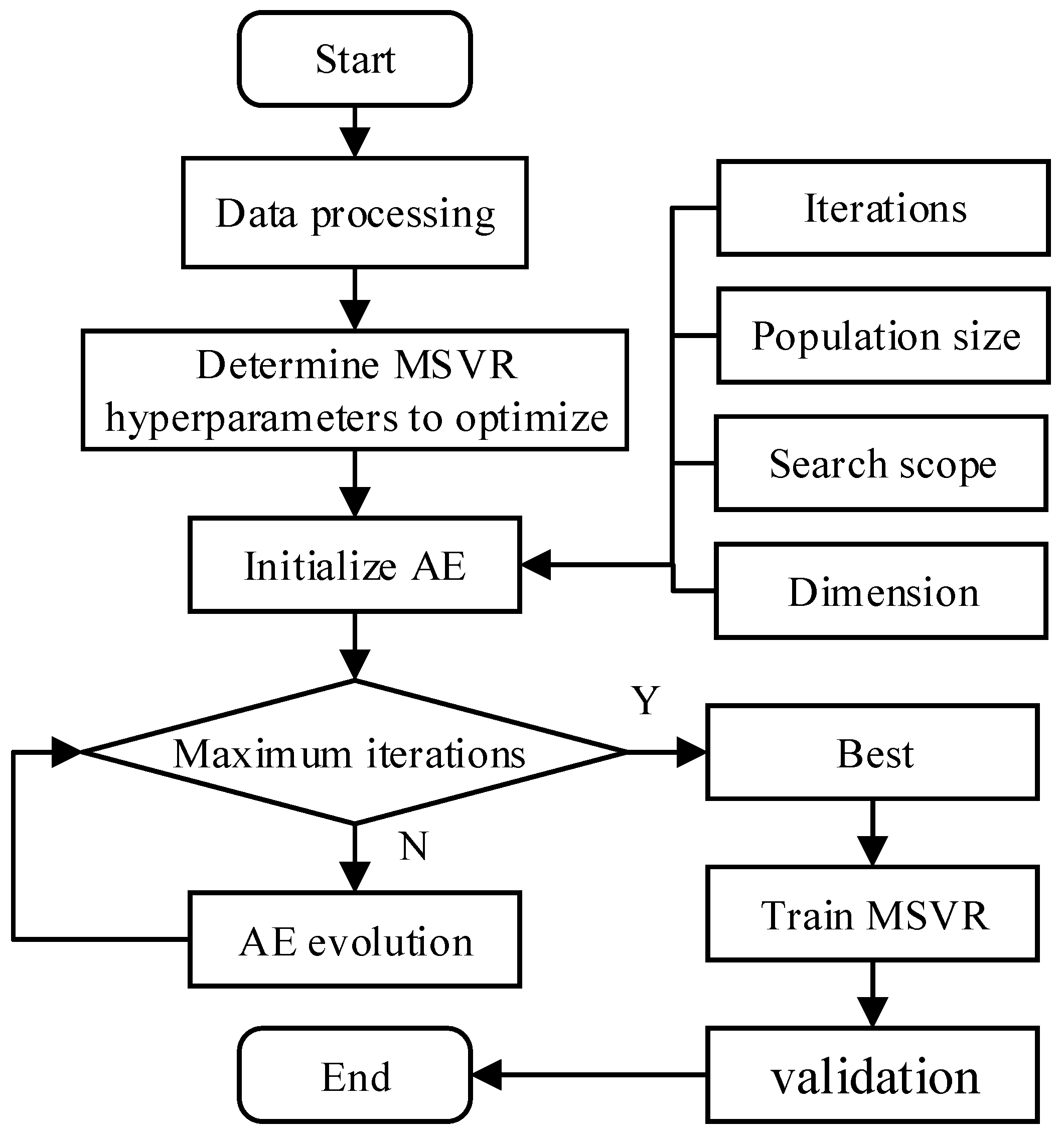
The regression performance of MSVR is highly dependent on the selection of its hyperparameters, and different kernel functions correspond to different kernel parameters and search ranges. Since it is difficult to accurately set these parameters through empirical methods to ensure regression accuracy, the excellent search performance of AE is used to automatically iterate and find the optimal target parameters. The choice of fitness function also affects the performance of AE. This paper selects the mean square error (MSE) as the fitness function. When the MSE value reaches the minimum, the corresponding hyperparameter value is optimal and corresponds to the highest regression accuracy. The steps of AE optimization of MSVR are as follows:

(1) Determine the optimization target and scope: Determine the hyperparameters and their ranges that need to be optimized for MSVR.

(2) Initialize AE: Set the maximum number of iterations, optimization dimension (i.e., the number of hyperparameters to be optimized), and population size of AE.

(3) Iterative optimization: Run AE until the maximum number of iterations is reached to obtain the optimal hyperparameters.

(4) MSVR model training: Use this optimal hyperparameter to train the MSVR model.

(5) Verification: Verify the generalization performance of the optimal MSVR model obtained through training by predicting unknown data.

The flowchart of AE-MSVR is shown in Figure 3.

4. Model Validation

4.1. Training Data

In 1965, Chislett et al. [31] systematically measured multiple hydrodynamic derivatives of a Mariner Class Vessel model in the Abkowitz model framework through planar motion mechanism (PMM) experiments. Their work successfully simulated real-world ship maneuvers, including spiral tests, turning circle tests, and zigzag tests. To ensure model accuracy and reliability, this study references the validation data obtained from Chislett et al.’s experiments.

Table 1. Main parameters of mariner.

Parameter	Value
Length overall ($L_{oa}$)	171.8 m
Length between perpendiculars ($L_{pp}$)	160.93 m
Maximum beam (B)	23.17 m
Design draft (T)	8.23 m
Design displacement (∇)	18,541 m3
Design speed ($U_0$)	15 kn (7.7175 m/s)

presents an outline of the ship’s fundamental characteristics.

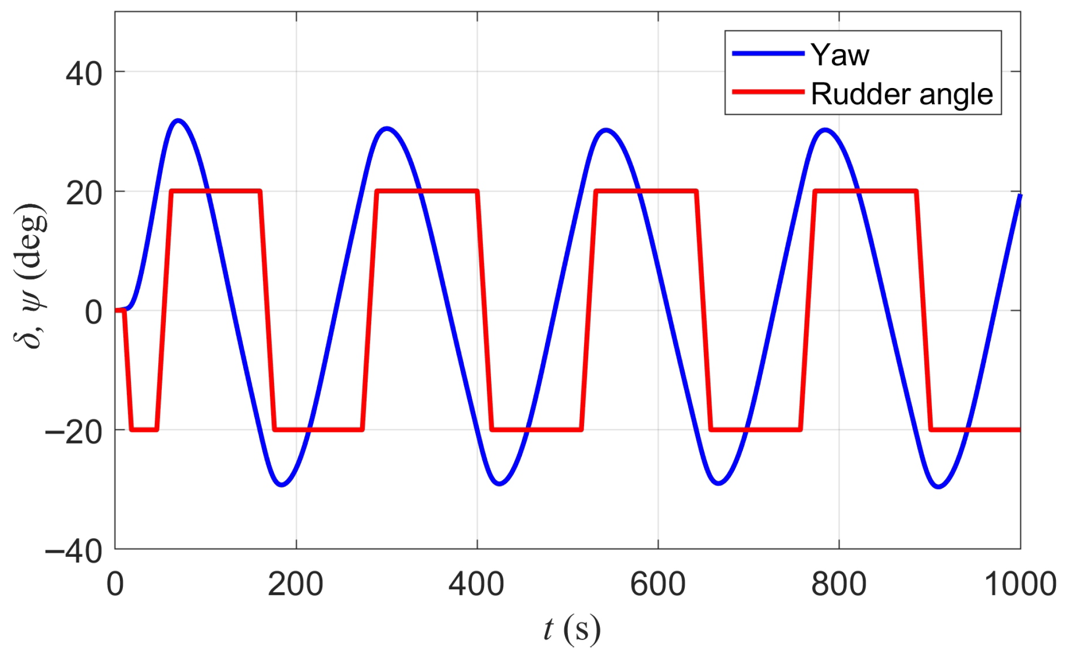
Ship motion simulation experiments can be easily performed in the Marine System Simulator (MSS). The platform facilitates diverse testing frameworks while providing robust computational resources for marine system modeling. Turning circle tests and zigzag tests are two primary categories of standard ship maneuvering tests. Due to the simplicity of turning motion conditions, they are unsuitable for generating training data. This study employs 20° and 10° zigzag test to generate the training dataset. The MSS is configured in detail as follows: the ship type is a mariner, the speed is 7.7175 m/s, the simulation duration is 1000 s, the execution time of steering begins at 10 s, the rudder angles are [20,20] and [10,10], and the data interval is 1 s. At the same time, record the motion variables (u,v,r,U) and rudder angle $\delta$ and save them. The 1000-sample dataset covers the entire zigzag test as illustrated in Figure 4 and Figure 5.

The following section verifies the sensitivity of the identification model based on Euler discretization as described in Section 2.2, to discrete step sizes. We generated 20° zigzag test data with varying time steps (h = 0.01, 0.1, 0.5, 1.0) in the simulator, with each dataset spanning 1000 s. To obtain an equal number of samples, all data were uniformly sampled at 1 s intervals, resulting in 1000 samples per dataset. This approach reflects the influence of integration step size on dynamics while ensuring consistent training dataset lengths. We generated 20° zigzag maneuver data using the MSS simulator with four different time intervals 0.01, 0.1, 0.5, 1, all sampled at a 1 s time interval. Using these four datasets, the hydrodynamic vectors $\mathit{A}$, $\mathit{B}$, $\mathit{C}$ were constructed, and the variance inflation factor (VIF) for each regression term of the matrix was calculated. The results are presented in

Table 2. VIF of data at different time intervals.

A	1 s	0.5 s	0.1 s	0.01 s	B	1 s	0.5 s	0.1 s	0.01 s
${\mathit{A}}_1$	127.1	127.9	129.0	129.4	${\mathit{B}}_1$	1118.1	1254.7	1354.2	1371.3
${\mathit{A}}_2$	873.5	875.2	880.1	882.2	${\mathit{B}}_2$	1506.4	1691.3	1838.1	1870.6
${\mathit{A}}_3$	384.5	383.8	385.3	386.1	${\mathit{B}}_3$	934.8	962.1	970.1	970.7
${\mathit{A}}_4$	214.9	229.3	234.0	233.4	${\mathit{B}}_4$	2182.4	2258.3	2270.7	2267.3
${\mathit{A}}_5$	220.2	233.8	240.7	241.9	${\mathit{B}}_5$	1812.5	1925.1	1975.1	1991.8
${\mathit{A}}_6$	8.8	9.3	10.0	10.0	${\mathit{B}}_6$	2894.5	3092.6	3170.9	3197.6
${\mathit{A}}_7$	9.8	10.2	10.5	10.5	${\mathit{B}}_7$	551.7	598.9	630	637.7
${\mathit{A}}_8$	777.0	828.7	844.7	843.2	${\mathit{B}}_8$	114.3	115.6	112.8	112.4
${\mathit{A}}_9$	61.9	62.9	63.3	63.7	${\mathit{B}}_9$	2349.2	2487.9	2566.6	2597.8
${\mathit{A}}_{10}$	29.1	29.0	29.1	29.3	${\mathit{B}}_{10}$	589.3	616.7	637.9	645.9
					${\mathit{B}}_{11}$	47.8	50.6	50.3	49.5
					${\mathit{B}}_{12}$	620.1	651.6	668.9	672.5
					${\mathit{B}}_{13}$	325	326.5	331.7	332
					${\mathit{B}}_{14}$	288.6	293.5	301.1	301.5
					${\mathit{B}}_{15}$	23.1	23.4	23.8	23.9

. Since vectors $\mathit{B}$ and $\mathit{C}$ are identical, only $\mathit{A}$ and $\mathit{B}$ are listed. The table indicates severe multicollinearity among the hydrodynamic forces for surge, sway, and yaw. The VIF values for surge hydrodynamics are significantly lower than those for sway and yaw. Among the different time intervals, the VIF is smallest for the 1 s interval, and as the time interval approaches 1 s, the VIF decreases, indicating weaker multicollinearity, which is more pronounced in vector $\mathit{B}$. Therefore, to enhance identification and modeling performance, subsequent sections adopt data generated by MSS with a 1 s time interval.

4.2. Identification Process

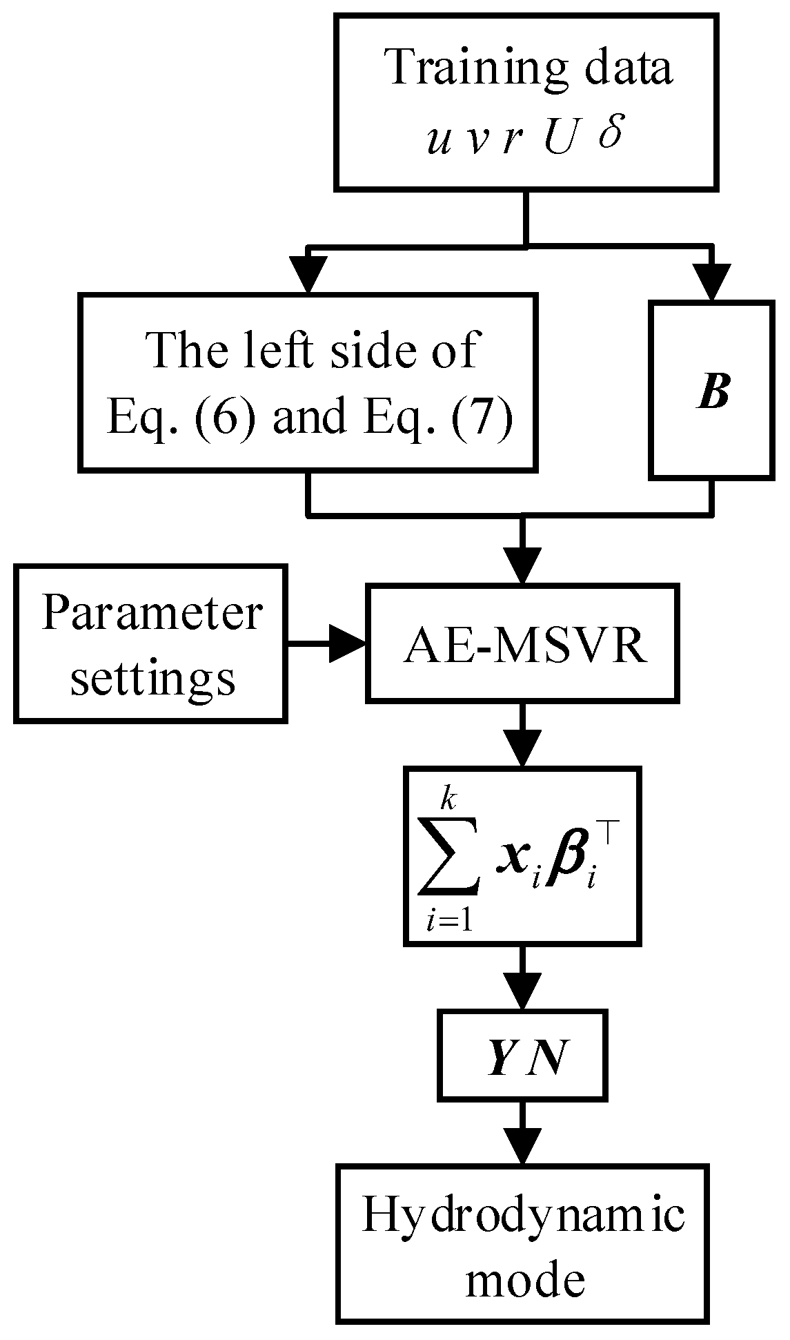
As we know from Section 2.2, the input vector $\mathit{B}$ and the left-hand side terms of the sway Equation (9) and the yaw Equation (10) can be obtained based on the training data. This input–output relationship is fitted via AE-MSVR, configured with the following: population = 50, max iterations = 30, the optimization dimension is 2 (corresponding to C and $ϵ$ of MSVR) and the search range is [0, 10,000] and [0, 10⁻³], respectively, and the objective function is Equation (25) (taking the Equations (9) and (10) as an example).

$$f\left(x_i\right)=\sum _{k=1}^n{({\widehat{y}}_k^1\left(x_i\right)-y_k^1)}^2+\sum _{k=1}^n{({\widehat{y}}_k^2\left(x_i\right)-y_k^2)}^2$$

(25)

$${\widehat{y}}_k^1\left(x_i\right)=Y^{\prime }\mathit{B}, {\widehat{y}}_k^2\left(x_i\right)=N^{\prime }\mathit{C}$$

where $x_i$ is a candidate hyperparameter (here, C and $ϵ$), $Y^{\prime }$ and $N^{\prime }$ are the weight coefficients (hydrodynamic derivatives) extracted after training MSVR with $x_i$, i.e., Equations (12) and (13); $\mathit{B}$ and $\mathit{C}$ are Equation (15); ${\widehat{y}}_k^1\left(x_i\right)$ and ${\widehat{y}}_k^2\left(x_i\right)$ are the left-hand-side values of Equations (9) and (10) calculated using the identified hydrodynamic derivatives, and $y_k^1$ and $y_k^2$ are the left-hand-side values of Equations (9) and (10) obtained from the training data; and n is the number of samples.

After the training is completed, the coefficients $\mathit{Y}$ and $\mathit{N}$ are extracted from the obtained MSVR model and substituted into Equations (9) and (10) to obtain the sway and yaw motion equations in the Abkowitz model. Figure 6 shows the modeling process. It should be noted that since the hydrodynamic derivatives of the surge motion equation need to be identified separately, the figure only shows the identification process of the sway and yaw motion equations.

4.3. Identification Results

Table 3. Hydrodynamic derivative identification results based on 20° zigzag test data ($\times {10}^{-5}$).

X	PMM	AE-MSVR	SVR	Y	PMM	AE-MSVR	SVR	N	PMM	AE-MSVR	SVR
$X_u^{\prime }$	−184	−183.9	−185.2	$Y_v^{\prime }$	−1160	−1160.0	−1158.2	$N_v^{\prime }$	−264	−264	−262.4
$X_{uu}^{\prime }$	−110	−109.4	−116.6	$Y_r^{\prime }$	−499	−499.0	−498.1	$N_r^{\prime }$	−166	−166	−165.4
$X_{uuu}^{\prime }$	−215	−212.9	−220.0	$Y_{vvv}^{\prime }$	−8078	−8080.0	−8150.4	$N_{vvv}^{\prime }$	1636	1638.7	1667.5
$X_{vv}^{\prime }$	−899	−898.8	−923.0	$Y_{vvr}^{\prime }$	15,356	15,354.2	15,312.0	$N_{vvr}^{\prime }$	−5483	−5481	−5484.0
$X_{rr}^{\prime }$	18	18	13.8	$Y_{vu}^{\prime }$	−1160	−1160.2	−1156.2	$N_{vu}^{\prime }$	−264	−263.8	−250.6
$X_{\delta \delta }^{\prime }$	−95	−95	−94.6	$Y_{ru}^{\prime }$	−499	−499.1	−497.3	$N_{ru}^{\prime }$	−166	−165.9	−162.2
$X_{\delta \delta u}^{\prime }$	−190	−190	−190.2	$Y_{\delta }^{\prime }$	278	278.0	277.6	$N_{\delta }^{\prime }$	−139	−139	−139.0
$X_{vr}^{\prime }$	798	798.1	779.3	$Y_{\delta \delta \delta }^{\prime }$	−90	−90.0	−89.6	$N_{\delta \delta \delta }^{\prime }$	45	45	42.3
$X_{v\delta }^{\prime }$	93	93	92.3	$Y_{\delta u}^{\prime }$	556	555.9	554.3	$N_{\delta u}^{\prime }$	−278	−277.9	−270.0
$X_{v\delta u}^{\prime }$	93	93	86.1	$Y_{\delta uu}^{\prime }$	278	277.8	271.7	$N_{\delta uu}^{\prime }$	−139	−138.8	−87.8
				$Y_{v\delta \delta }^{\prime }$	−4	−3.9	−3.6	$N_{v\delta \delta }^{\prime }$	13	13	17.5
				$Y_{vv\delta }^{\prime }$	1190	1189.0	1213.1	$N_{vv\delta }^{\prime }$	−489	−488.2	−476.2
				$Y_0^{\prime }$	−4	−4.0	−3.6	$N_0^{\prime }$	3	3	1.6
				$Y_{0u}^{\prime }$	−8	−8.0	−8.6	$N_{0u}^{\prime }$	6	6	8.0
				$Y_{0uu}^{\prime }$	−4	−4.0	−2.7	$N_{0uu}^{\prime }$	3	3	−0.4

and

Table 4. Hydrodynamic derivative identification results based on 10° zigzag test data ($\times {10}^{-5}$).

X	PMM	AE-MSVR	Y	PMM	AE-MSVR	N	PMM	AE-MSVR
$X_u^{\prime }$	−184	−183.96	$Y_v^{\prime }$	−1160	−1159.95	$N_v^{\prime }$	−264	−264.04
$X_{uu}^{\prime }$	−110	−108.55	$Y_r^{\prime }$	−499	−498.97	$N_r^{\prime }$	−166	−166.02
$X_{uuu}^{\prime }$	−215	−202.21	$Y_{vvv}^{\prime }$	−8078	−8080.85	$N_{vvv}^{\prime }$	1636	1644.69
$X_{vv}^{\prime }$	−899	−898.95	$Y_{vvr}^{\prime }$	15,356	15,352.17	$N_{vvr}^{\prime }$	−5483	−5477.4
$X_{rr}^{\prime }$	18	18	$Y_{vu}^{\prime }$	−1160	−1160.59	$N_{vu}^{\prime }$	−264	−263.31
$X_{\delta \delta }^{\prime }$	−95	−94.99	$Y_{ru}^{\prime }$	−499	−499.48	$N_{ru}^{\prime }$	−166	−165.58
$X_{\delta \delta u}^{\prime }$	−190	−189.86	$Y_{\delta }^{\prime }$	278	278.01	$N_{\delta }^{\prime }$	−139	−139.01
$X_{vr}^{\prime }$	798	798.02	$Y_{\delta \delta \delta }^{\prime }$	−90	−90	$N_{\delta \delta \delta }^{\prime }$	45	45.04
$X_{v\delta }^{\prime }$	93	93	$Y_{\delta u}^{\prime }$	556	555.46	$N_{\delta u}^{\prime }$	−278	−277.66
$X_{v\delta u}^{\prime }$	93	93.11	$Y_{\delta uu}^{\prime }$	278	273.64	$N_{\delta uu}^{\prime }$	−139	−136.86
			$Y_{v\delta \delta }^{\prime }$	−4	−3.93	$N_{v\delta \delta }^{\prime }$	13	12.88
			$Y_{vv\delta }^{\prime }$	1190	1186.86	$N_{vv\delta }^{\prime }$	−489	−486.02
			$Y_0^{\prime }$	−4	−4	$N_0^{\prime }$	3	3
			$Y_{0u}^{\prime }$	−8	−7.97	$N_{0u}^{\prime }$	6	5.98
			$Y_{0uu}^{\prime }$	−4	−3.59	$N_{0uu}^{\prime }$	3	2.72

present the results of dimensionless hydrodynamic derivative identification using the 20° and 10° zigzag tests as training data. The tables show that the identification results based on the AE-MSVR for both maneuvering data agree well with the PMM test. However, because the 20° zigzag test more fully excites the ship’s motion, the identification results are superior to those of the 10° zigzag test. Table 3 also compares the identification results with those of the single-output SVR [13], demonstrating that nearly every hydrodynamic derivative is more accurate. It is noted that acceleration derivatives are treated as known constants in the identification process: $X_{\dot{u}}^{\prime }=-42\times {10}^{-5}$, $Y_{\dot{v}}^{\prime }=-748\times {10}^{-5}$, $Y_{\dot{r}}^{\prime }=-9.354\times {10}^{-5}$, $N_{\dot{v}}^{\prime }=4.646\times {10}^{-5}$, $N_{\dot{r}}^{\prime }=-43.8\times {10}^{-5}$, and other non-dimensional parameters involved in calculations include $m^{\prime }=798\times {10}^{-5}$, $I_z^{\prime }=39.2\times {10}^{-5}$, $x_G^{\prime }=-2300\times {10}^{-5}$.

4.4. Identified Model Validation

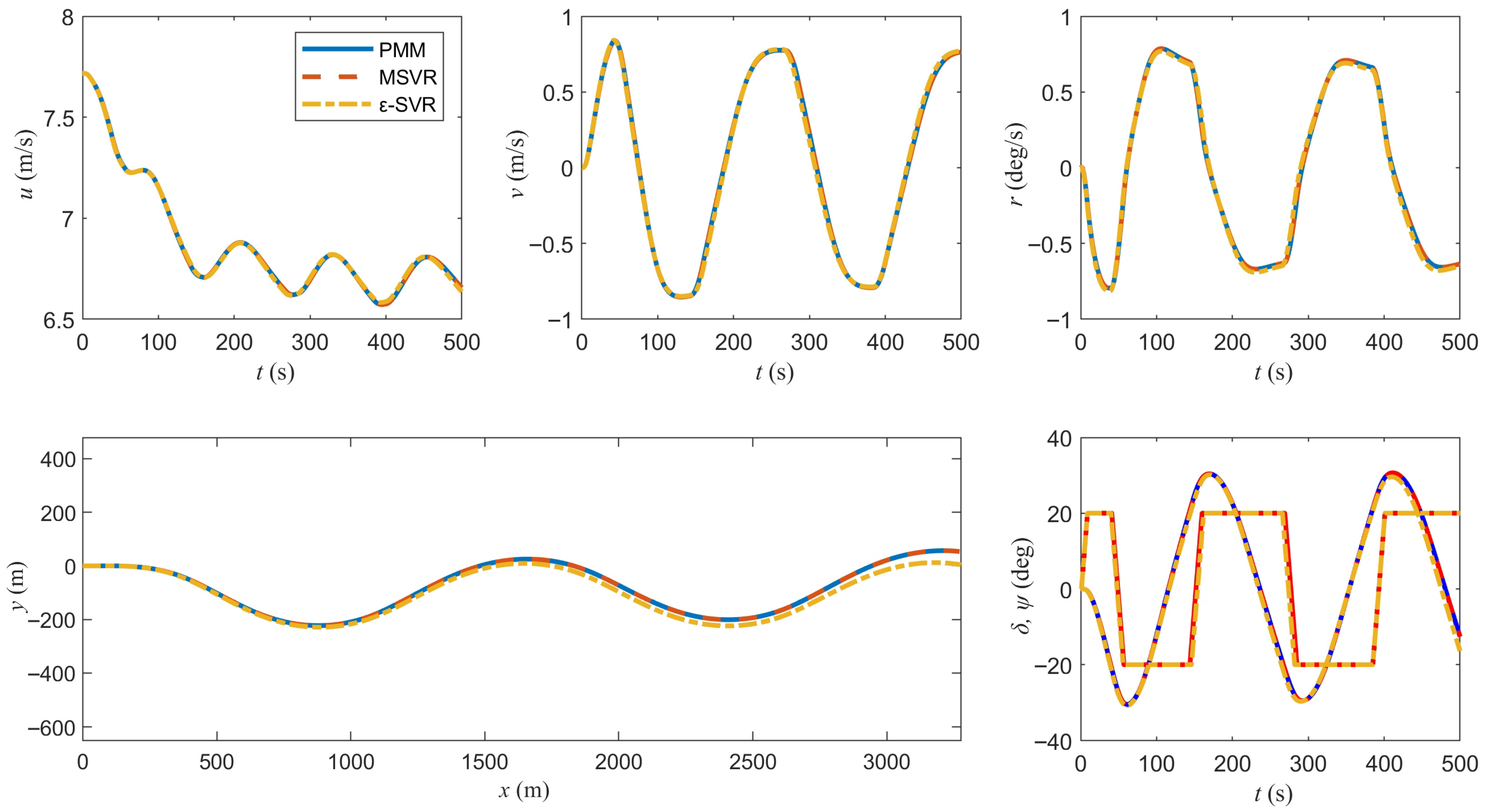
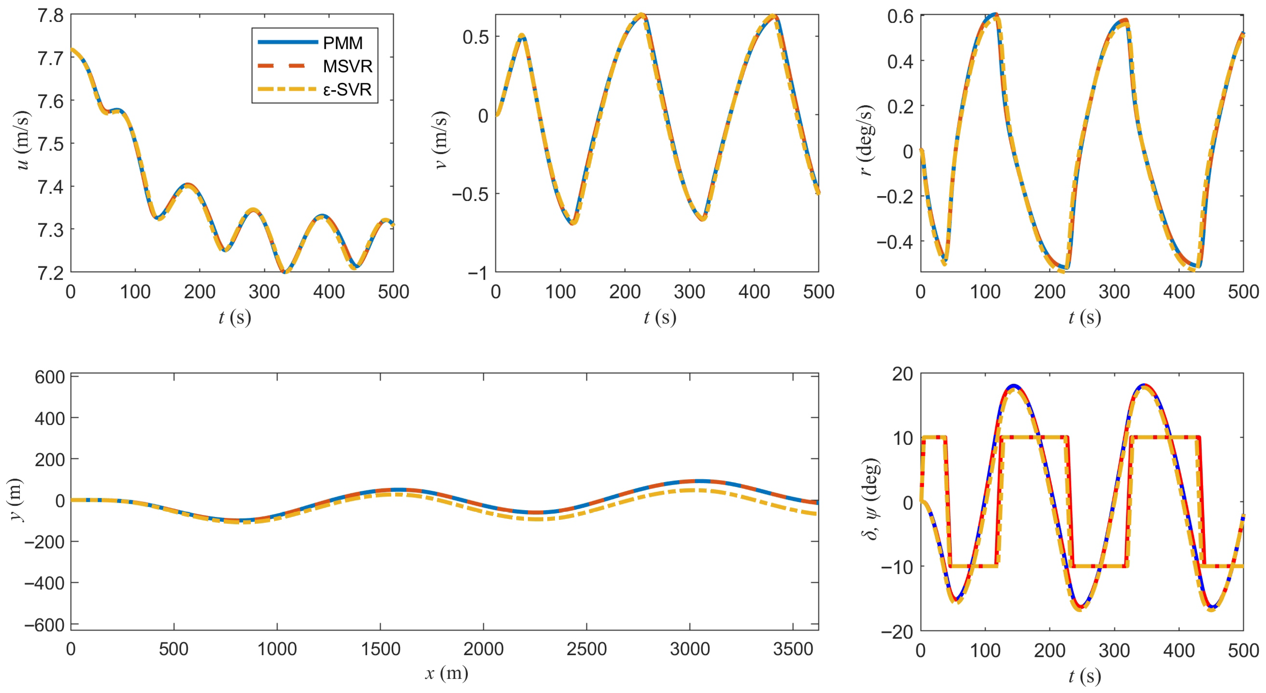
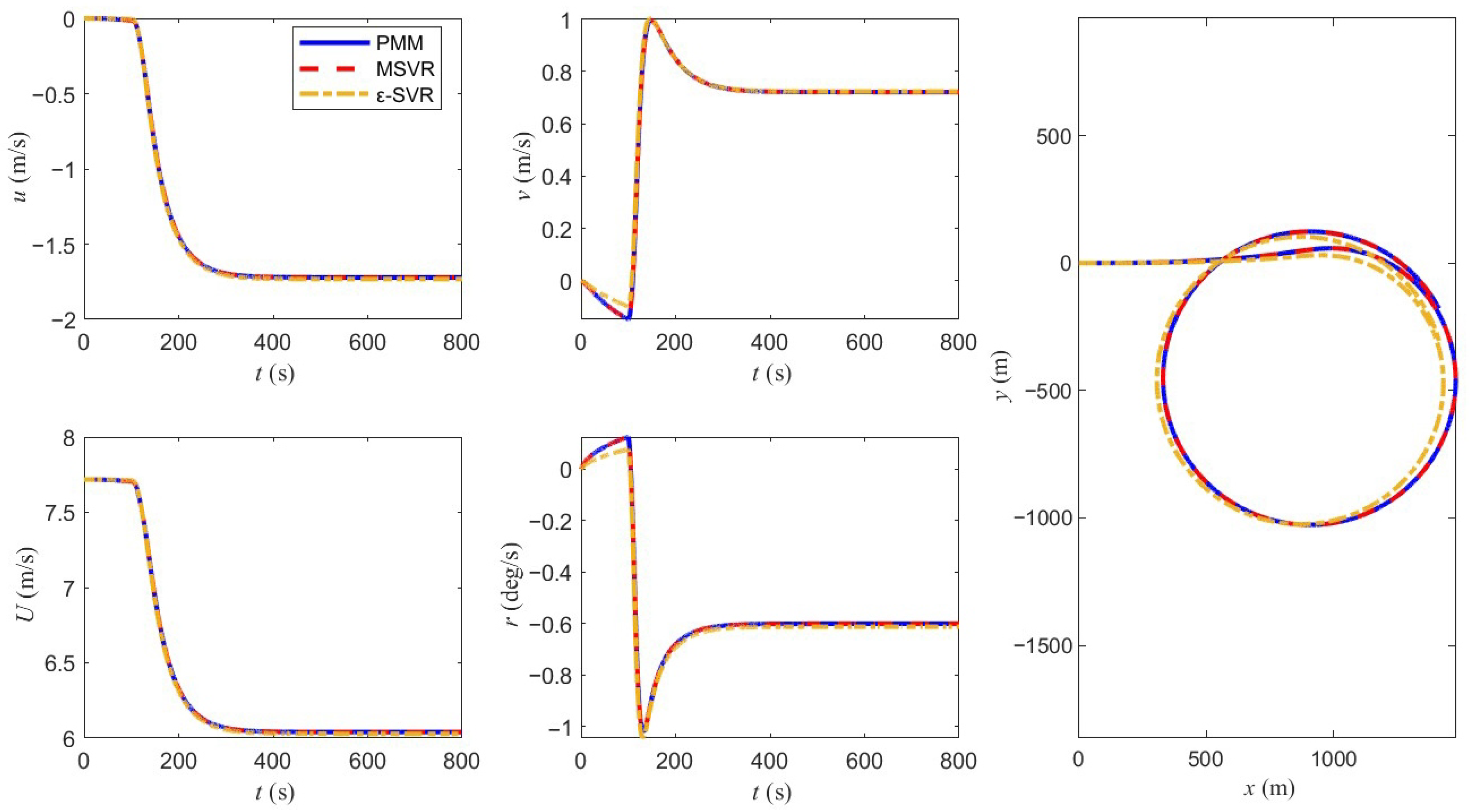
A key criterion for evaluating the applicability of the model is to generalize to untrained maneuvering scenarios. To verify the performance of the obtained hydrodynamic model, numerical simulations were used to predict the 20°/20° and 10°/10° zigzag tests and the 35° turning circle test. Figure 7, Figure 8 and Figure 9 compare the results of the reference model, the single-output SVR identification model, and the AE-MSVR identification model in these three maneuvering tests. Although differences in u, v, r, and heading angle $\psi$ may be difficult to distinguish directly, the trajectory comparison (where errors accumulate) clearly demonstrates that AE-MSVR achieves closer agreement with the reference model than single-output SVR. This superiority is particularly conspicuous in the 35° turning circle test. For the purpose of evaluating model performance, MSE and correlation coefficient (CC) are used to measure the prediction accuracy. CC can measure the trend consistency between the predicted value and the true value, and MSE measures the absolute error between the predicted value and the true value. MSE and CC are defined as Equations (26) and (27):

$$\mathrm{MSE}={\displaystyle \frac{1}{n}}\sum _{k=1}^n{\left[act\left(k\right)-pre\left(k\right)\right]}^2$$

(26)

$$CC={\displaystyle \frac{{\displaystyle \sum _{k=1}^{\mathrm{n}}}\left(pre\left(k\right)-\overline{pre}\right)\left(act\left(k\right)-\overline{act}\right)}{\sqrt{{\displaystyle \sum _{k=1}^n}{\left(pre\left(k\right)-\overline{pre}\right)}^2\sqrt{{\displaystyle \sum _{k=1}^n}{\left(act\left(k\right)-\overline{act}\right)}^2}}}}$$

(27)

where $pre$ and $\overline{pre}$ represent the predicted results and the average value, $act$ and $\overline{act}$ represent the actual results and the average value, and n is the data length.

The AE-MSVR and SVR identification results based on the 20° zigzag test in Table 3 are substituted into Equation (5) to perform various manipulation motion simulations.

Table 5. Comparison of the prediction accuracy.

		MSE		CC
		AE-MSVR	SVR	AE-MSVR	SVR
20°Z	u	4.56 × 10−11	6.12 × 10−5	0.9999	0.9996
	v	1.05 × 10−14	2.13 × 10−7	0.9999	0.9990
	r	1.89 × 10−11	5.02 × 10−4	0.9999	0.9993
10°Z	u	4.16 × 10−10	3.29 × 10−5	0.9999	0.9992
	v	6.97 × 10−14	2.79 × 10−7	0.9999	0.9968
	r	2.32 × 10−10	6.75 × 10−4	0.9999	0.9984
35°T	u	1.44 × 10−7	1.27 × 10−4	0.9999	0.9999
	v	9.80 × 10−9	2.37 × 10−4	0.9999	0.9995
	r	5.69 × 10−9	3.51 × 10−4	0.9999	0.9995

lists the MSE and CC of the simulation results relative to the reference model for u, v, and r responses. Analysis of the table shows that the MSE of u, v, and r obtained by the AE-MSVR identification model are several orders of magnitude lower than those of the SVR identification model, and its CC value is as high as 0.9999, which is also significantly better than SVR. These results show that the AE-MSVR identification method performs better than SVR, and its results are highly consistent with the reference model.

5. Model Identification Under Disturbance

5.1. Disturbance Model

Table 3 and Table 4 indicate that the hydrodynamic derivatives identified exhibit good agreement with the PMM test, and validate the effectiveness of the modeling approach. However, actual experimental training samples exhibit noise when compared to simulated samples, stemming from sensor errors and inherent environmental uncertainties like wind, waves, and currents. This study adopts the disturbance model Equation (28) proposed by Sutulo [32]:

$${\zeta }_i={\zeta }_{0i}+max\left(\zeta \right){\xi }_i{k}_0{k}_{\zeta }$$

(28)

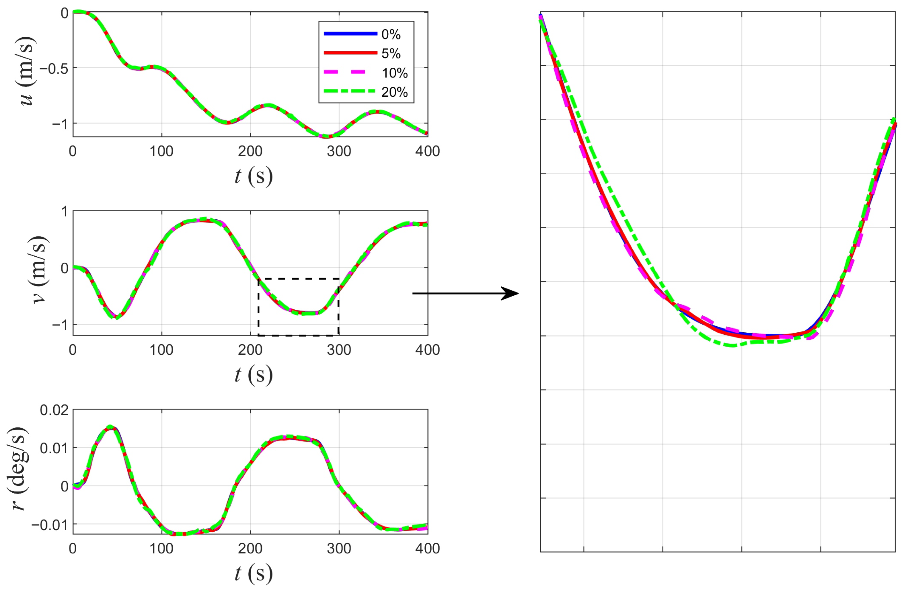
where $\zeta \in \{u,v,r\}$ denotes the motion parameters, ${\zeta }_{0i}$ is the original data, max($\zeta$) represents the maximum absolute value, and $k_0$ globally controls the noise intensity to represent different levels of noise. ${\xi }_i$ represents a Gaussian-distributed random variable (variance: 0.2). $k_{\zeta }$ operates as a dedicated scaling factor. Given that the noise of u is significantly less than that of v and that of r, we set $k_{\zeta }$ = 0.2 for u and $k_{\zeta }$ = 1.0 for v and r. The comparison of the original data and polluted data ($k_0$ = 5%, 10%, 20%) is shown in Figure 10. For clarity, only part of the data is displayed.

5.2. Identification Under Disturbance

When directly identifying hydrodynamic derivatives from polluted data, substantial deviations in results often occur. Therefore, wavelet denoising is utilized for preprocessing and smoothing the training dataset. Set DB4 as the wavelet base; the number of decomposition layers is 5; and the threshold function is Bayes. The effect of denoising is shown in Figure 11.

The parameter identification process for maneuvering data containing disturbances is the same as that in Section 4.2. The AE-MSVR algorithm was applied to identify parameters using the denoised training dataset. To mitigate random fluctuations, each experiment was repeated 50 times, and the average result was adopted. A 35° turning circle test served to verify the robustness of the identified model. Figure 12 plots comparative simulation results for u, v, r, $\psi$, and ship trajectory (x, y) between the identification and reference model. It can be observed that, even under disturbance, the identified model effectively captures the dynamic properties of the ship and generates a relatively accurate response. At disturbance levels of $k_0$ = 5% and 10%, the prediction errors remain within an acceptable range. Generally, higher levels of disturbance lead to greater deviations. When the disturbance level $k_0$ increases to 20%, not only does the result deviation become larger but it also becomes unstable. This is primarily due to the data becoming highly distorted at this interference level, making it challenging for the denoising method to completely filter out the noise.

Turning circle maneuvering characteristics serve as quantitative error indicators. These calculated values, detailed in

Table 6. Maneuvering characteristics and deviation percentage of the identified model.

Maneuvering Characteristics	Reference Value (m)	5%		10%		20%
		Value (m)	Deviation (%)	Value (m)	Deviation (%)	Value (m)	Deviation (%)
Steady turning radius	576	587	2.0	533	−7.4	453	−21.3
Maximum transfer	1028	1050	2.1	985	−4.2	770	−25.0
Maximum advance	710	715	0.7	750	5.6	661	−6.8
Transfer at 90 (deg) heading	385	399	3.6	373	−3.1	283	−26.6
Advance at 90 (deg) heading	705	710	0.8	745	5.7	659	−6.5
Tactical diameter at 180 (deg) heading	1023	1045	2.2	980	−4.1	768	−24.9

, reveal that the deviation is less than 3.6% at $k_0$ = 5%, less than 7.4% at $k_0$ = 10%, and reaches a maximum of 26.6% at $k_0$ = 20%. From the above results, we can see that under mild or moderate environments, the identified model sustains key characteristics precision provides acceptable predictive performance. Although the maneuvering characteristics exhibit significant deviations under harsh environment, the model still demonstrates the capability to predict short-term trajectories. The results demonstrate that the AE-MSVR-based method can achieve relatively accurate parameter identification in low-interference environments. However, such noise levels rarely occur in actual tests, so the 20% scenario should be considered an extreme test to demonstrate the robustness boundary. During actual maneuvering tests, external environmental interference should be minimized, or training data from actual operations in calm waters should be used. The results show that the ship motion mathematical model identification method based on AE-MSVR can accurately identify the model in a low-disturbance environment.

6. Conclusions

(1) This paper addresses the strong coupling between yaw and sway motion in the ship motion model by proposing an AE-MSVR identification method for ship motion modeling. This method approaches the yaw and sway motion equations as a MIMO problem, utilizing MSVR for modeling and optimizing hyperparameters with AE. It reduces parameter drift by restructuring the regression model’s input–output.

(2) The ship motion state data is obtained by simulating 20° zigzag maneuver. The model is trained using this data. The results show that the AE-MSVR identification method provides promising estimations of the linear and nonlinear hydrodynamic derivatives within a 3-DOF Abkowitz model. The identified hydrodynamic derivatives exhibit high agreement with PMM test results, yielding significantly improved accuracy over single-output SVR.

(3) Different levels of disturbance are introduced into the training data to simulate actual measurement errors and complex environments. Calculation of the maneuvering characteristics from the turning circle test demonstrates that this method can achieve reliable identification in a low-disturbance environment.

The AE-MSVR identification method proposed in this paper can not only identify the complex hydrodynamic derivatives of ships with promising accuracy but also maintain good robustness under the interference of data noise, which provides an effective way for predicting ship motion and maneuverability.

While the proposed AE-MSVR framework has demonstrated promising results in identifying hydrodynamic derivatives and predicting maneuvering performance, several limitations should be acknowledged. First, the training data were based on simulated zigzag maneuvers. Although simulations provide controllable and repeatable conditions, the absence of real free-running trials limits the immediate applicability to practice. Second, the disturbance model was restricted to Gaussian noise, which represents a simplification since real maneuvering trials often involve non-Gaussian disturbances such as colored processes. Third, although this paper reduces parameter drift by adopting a regression model that reconstructs input and output, this phenomenon will be aggravated when interference is added, reducing accuracy.

Future work will focus on the following:

(1) Validating the identification method presented in this paper using data from free-running model tests conducted at the Hamburg Ship Model Basin (HSVA);

(2) Extending the robustness analysis to non-Gaussian noise modeling and computing confidence intervals;

(3) Introducing adaptive or hybrid modeling methods to mitigate parameter drift and improve model generalization.

References

1. IMO. Interim Guidelines on the Second Generation Intact Stability Criteria; Technical Report MSC.1/Circ.1627; IMO: London, UK, 2020. [Google Scholar]
2. Skulstad, R.; Li, G.; Fossen, T.I.; Vik, B.; Zhang, H. A hybrid approach to motion prediction for ship docking-integration of a neural network model into the ship dynamic model. IEEE Trans. Instrum. Meas. 2021, 70, 2501311. [Google Scholar] [CrossRef]
3. Abkowitz, M.A. Lectures on Ship Hydrodynamics–Steering and Manoeuvrability; Report No. Hy-5; Hydro- and Aerodynamics Laboratory: Lyngby, Denmark, 1964. [Google Scholar]
4. Xia, H.; Ji, Y.; Xu, L.; Alsaedi, A.; Hayat, T. Maximum likelihood-based gradient estimation for multivariable nonlinear systems using the multiinnovation identification theory. Int. J. Robust Nonlinear Control. 2020, 30, 5446–5463. [Google Scholar] [CrossRef]
5. Xue, Y.; Liu, Y.; Ji, C.; Xue, G. Hydrodynamic parameter identification for ship manoeuvring mathematical models using a Bayesian approach. Ocean. Eng. 2020, 195, 106612. [Google Scholar] [CrossRef]
6. Zhong, Y.; Yu, C.; Wang, R.; Pei, T.; Lian, L. Adaptive anti-noise least-squares algorithm for parameter identification of unmanned marine vehicles: Theory, simulation, and experiment. Int. J. Fuzzy Syst. 2023, 25, 369–381. [Google Scholar] [CrossRef]
7. Wakita, K.; Maki, A.; Umeda, N.; Miyauchi, Y.; Shimoji, T.; Rachman, D.M.; Akimoto, Y. On neural network identification for low-speed ship maneuvering model. J. Mar. Sci. Technol. 2022, 27, 772–785. [Google Scholar] [CrossRef]
8. Perez, T.; Fossen, T.I. Practical aspects of frequency-domain identification of dynamic models of marine structures from hydrodynamic data. Ocean. Eng. 2011, 38, 426–435. [Google Scholar] [CrossRef]
9. Meng, Y.; Zhang, X.; Zhang, X.; Ma, D.; Duan, Y. Online ship motion identification modeling and its application to course-keeping control. Ocean. Eng. 2024, 294, 116853. [Google Scholar] [CrossRef]
10. Vapnik, V. An overview of statistical learning theory. IEEE Trans. Neural Netw. 1999, 10, 988–999. [Google Scholar] [CrossRef]
11. Wang, X.; Zou, Z.; Yu, L.; Cai, W. System identification modeling of ship manoeuvring motion in 4 degrees of freedom based on support vector machines. China Ocean. Eng. 2015, 29, 519–534. [Google Scholar] [CrossRef]
12. Luo, W.L.; Zou, Z.J. Parametric Identification of Ship Maneuvering Models by Using Support Vector Machines. J. Ship Res. 2009, 53, 19–30. [Google Scholar] [CrossRef]
13. Wang, T.; Li, G.; Wu, B.; Æsøy, V.; Zhang, H. Parameter identification of ship manoeuvring model under disturbance using support vector machine method. Ships Offshore Struct. 2021, 16, 13–21. [Google Scholar] [CrossRef]
14. Xu, H.; Hassani, V.; Guedes Soares, C. Comparing generic and vectorial nonlinear manoeuvring models and parameter estimation using optimal truncated least square support vector machine. Appl. Ocean. Res. 2020, 97, 102061. [Google Scholar] [CrossRef]
15. Xu, H.; Guedes Soares, C. Hydrodynamic coefficient estimation for ship manoeuvring in shallow water using an optimal truncated LS-SVM. Ocean. Eng. 2019, 191, 106488. [Google Scholar] [CrossRef]
16. Xu, P.; Cao, Q.; Shen, Y.; Chen, M.; Ding, Y.; Ding, Y. Predicting the motion of a USV using support vector regression with mixed kernel function. J. Mar. Sci. Eng. 2022, 10, 1899. [Google Scholar] [CrossRef]
17. Chen, L.; Yang, P.; Li, S.; Tian, Y.; Liu, G.; Hao, G. Grey-box identification modeling of ship maneuvering motion based on LS-SVM. Ocean. Eng. 2022, 266, 112957. [Google Scholar] [CrossRef]
18. Hu, Y.; Song, L.; Liu, Z.; Yao, J. Identification of ship hydrodynamic derivatives based on LS-SVM with wavelet threshold denoising. J. Mar. Sci. Eng. 2021, 9, 1356. [Google Scholar] [CrossRef]
19. Tuia, D.; Verrelst, J.; Alonso, L.; Perez-Cruz, F.; Camps-Valls, G. Multioutput support vector regression for remote sensing biophysical parameter estimation. IEEE Geosci. Remote. Sens. Lett. 2011, 8, 804–808. [Google Scholar] [CrossRef]
20. Sanchez-Fernandez, M.; de Prado-Cumplido, M.; Arenas-Garcia, J.; Perez-Cruz, F. SVM multiregression for nonlinear channel estimation in multiple-input multiple-output systems. IEEE Trans. Signal Process. 2004, 52, 2298–2307. [Google Scholar] [CrossRef]
21. Jiang, L.; Shang, X.; Jin, B.; Zhang, Z.; Zhang, W. Black-box modeling of ship maneuvering motion using multi-output least-squares support vector regression based on optimal mixed kernel function. Ocean. Eng. 2024, 293, 116663. [Google Scholar] [CrossRef]
22. Zhang, Y.Y.; Wang, Z.H.; Zou, Z.J. Black-box modeling of ship maneuvering motion based on multi-output nu-support vector regression with random excitation signal. Ocean. Eng. 2022, 257, 111279. [Google Scholar] [CrossRef]
23. Li, S.; Yang, X.; Ren, H.; Li, C.; Feng, X. Non-parametric identification modeling and prediction of intelligent ship maneuvering motion based on real ship test at sea. Ocean. Eng. 2025, 330, 121267. [Google Scholar] [CrossRef]
24. Dong, Z.; Ding, Y.; Liu, W.; Hu, Z.; Lu, S.; Liu, Y. Maneuverability parameter identification of a water-jet USV based on truncated weighted LSSVM integrated with adaptive mutation PSO algorithm. Ocean. Eng. 2025, 321, 120474. [Google Scholar] [CrossRef]
25. Zhang, X.; Meng, Y.; Liu, Z.; Zhu, J. Modified grey wolf optimizer-based support vector regression for ship maneuvering identification with full-scale trial. J. Mar. Sci. Technol. 2022, 27, 576–588. [Google Scholar] [CrossRef]
26. Tian, R.; Zhang, X.; Liu, X. Identification modeling of ship manoeuvring motion based on ISSA-SVR. Ocean. Eng. 2024, 313, 119364. [Google Scholar] [CrossRef]
27. Gao, H.; Zhang, Q. Alpha evolution: An efficient evolutionary algorithm with evolution path adaptation and matrix generation. Eng. Appl. Artif. Intell. 2024, 137, 109202. [Google Scholar] [CrossRef]
28. Luo, W.; Li, X. Measures to diminish the parameter drift in the modeling of ship manoeuvring using system identification. Appl. Ocean. Res. 2017, 67, 9–20. [Google Scholar] [CrossRef]
29. Wang, X.; Zou, Z.; Hou, X.; Xu, F. System identification modelling of ship manoeuvring motion based on ɛ-support vector regression. J. Hydrodyn. 2015, 27, 502–512. [Google Scholar] [CrossRef]
30. Pérez-Cruz, F.; Vázquez, A.N.; Alarcón-Diana, P.L.; Artés-Rodríguez, A. An IRWLS procedure for SVR. In Proceedings of the 2000 10th European Signal Processing Conference, Tampere, Finland, 4–8 September 2000; pp. 1–4. [Google Scholar]
31. Chislett, M.; Strom-Tejsen, J. Planar motion mechanism tests and full-scale steering and manoeuvring predictions for a Mariner class vessel. Int. Shipbuild. Prog. 1965, 12, 201–224. [Google Scholar] [CrossRef]
32. Sutulo, S.; Guedes Soares, C. An algorithm for offline identification of ship manoeuvring mathematical models from free-running tests. Ocean. Eng. 2014, 79, 10–25. [Google Scholar] [CrossRef]
Figure 1. Two coordinate systems.
Jmse 13 01942 g001
Figure 2. The flowchart of AE.
Jmse 13 01942 g002
Figure 3. The flowchart of AE-MSVR.
Jmse 13 01942 g003
Figure 4. Training data for 20° zigzag test.
Jmse 13 01942 g004
Figure 5. Training data for 10° zigzag test.
Jmse 13 01942 g005
Figure 6. Identification flowchart.
Jmse 13 01942 g006
Figure 7. Comparison of 20°/20° zigzag test.
Jmse 13 01942 g007
Figure 8. Comparison of 10°/10° zigzag test.
Jmse 13 01942 g008
Figure 9. Comparison of 35° turning circle test.
Jmse 13 01942 g009
Figure 10. Partial data with different levels of disturbance.
Jmse 13 01942 g010
Figure 11. Denoised partial velocity data.
Jmse 13 01942 g011
Figure 12. Comparison of 35° turning circle test between the identified model and the reference model at different disturbance levels.
Jmse 13 01942 g012