Abstract
Traditional maritime target element resolution, relying on manual experience and uniform sampling, lacks accuracy and efficiency in non-uniform sampling, missing data, and noisy scenarios. While large language models (LLMs) offer a solution, their general knowledge gaps with maritime needs limit direct application. This paper proposes a fine-tuned LLM-based adaptive optimization method for non-uniform sampling maritime target element resolution, with three key novelties: first, selecting Doubao-Seed-1.6 as the base model and conducting targeted preprocessing on maritime multi-source data to address domain adaptation gaps; second, innovating a “Prefix tuning + LoRA” hybrid strategy (encoding maritime rules via Prefix tuning, freezing 95% of base parameters via LoRA to reduce trainable parameters to <0.5%) to balance cost and performance; third, building a non-uniform sampling-model collaboration mechanism, where the fine-tuned model dynamically adjusts the sampling density via semantic understanding to solve random sampling’s “structural information imbalance”. Experiments in close, away, and avoid scenarios (vs. five control models including original LLMs, rule-only/models, and ChatGPT-4.0) show that the proposed method achieves a comprehensive final score of 0.8133—37.1% higher than the sub-optimal data-only model (0.5933) and 87.7% higher than the original general model (0.4333). In high-risk avoid scenarios, its Top-1 Accuracy (0.7333) is 46.7% higher than the sub-optimal control, and Scene-Sensitive Recall (0.7333) is 2.2 times the original model; in close and away scenarios, its Top-1 Accuracy reaches 0.8667 and 0.9000, respectively. This method enhances resolution accuracy and adaptability, promoting LLM applications in navigation.
1. Introduction
With the rapid development of science and technology and the deepening of human exploration of the ocean, maritime activities are becoming more and more frequent. The resolution technology of maritime target elements emerges as the times require and has become one of the core technologies to ensure navigation safety. In the field of maritime safety, accurate and timely interpretation of maritime target elements is an important prerequisite to avoid ship collisions and ensure navigation safety.
Traditional maritime target element extraction methods are usually based on the ideal assumptions of complete time-series data, uniform sampling, and low noise. However, in practical applications, limited by the hardware performance of observation equipment, the complex marine environment, and the variability of remote communication links, the acquired maritime target time-series data often have serious data quality problems, which bring serious challenges to the resolution and robustness of the resolution methods. From the device level, the hardware limitation of the sampling frequency of the sensor and the inherent deviation in the positioning accuracy lead to the phenomenon of non-uniform sampling of the data, and the sampling interval fluctuates between seconds and minutes, which seriously destroys the time-series continuity of the data [1,2]. Under the influence of environmental factors, electromagnetic interference caused by adverse weather at sea (such as typhoons and rainstorms), as well as the absorption and attenuation of signals by seawater, will cause a large amount of data to go missing and even data gaps in some monitoring periods, resulting in the loss of key feature information [3]. This phenomenon often leads to the “data empty window” part of the monitoring period, which makes it difficult to accurately reconstruct the motion state and behavior characteristics of the target. At the same time, due to the interference of ionosphere, network congestion and other factors in the marine environment, noise signals such as impulse noise and white noise are easily mixed in the process of remote data transmission [4,5]. The interweaving and superposition of these problems make it difficult for traditional solution methods based on the assumption of uniform sampling to effectively extract the elements of target motion, which brings serious challenges to maritime target monitoring and situation analysis.
With the rapid development of artificial intelligence technology, deep learning technology has been gradually applied to the field of marine target element analysis. Its powerful feature-learning and pattern-recognition capabilities have brought new solutions for marine target element analysis. However, existing deep learning models still face some challenges when dealing with marine target element resolution tasks, such as insufficient generalization ability [6] and poor adaptability to complex backgrounds [7].
As an important breakthrough in the field of artificial intelligence, large language models have learned rich language knowledge and common sense through self-supervised learning on large-scale unlabeled text data and have powerful language understanding and generation capabilities. The application of large language models in the field of maritime object detection can provide new ideas for solving the limitations of traditional methods and existing deep learning models. By fine-tuning the large language model, it can better adapt to the needs of maritime object detection tasks and improve the accuracy and efficiency of detection.
Large language models have rapidly evolved in recent years. Starting from GPT-2 to GPT-4 [8], major players like Google, Anthropic, and Meta have launched models such as Gemini [9], Opus [10], and Llama-3 [11]. Built on Transformer architecture and pre-trained on vast corpora, these LLMs master language knowledge and semantic representation, excelling in traditional NLP tasks (text classification [12], sentiment analysis [13], translation [14]) and complex applications (text generation [14], code writing [15]).
Recent breakthroughs have further expanded the capabilities of large language models (LLMs). OpenAI’s GPT-5, released in August 2025, features enhanced multimodal integration, enabling seamless processing of text, images, and sensor data (e.g., maritime radar) while delivering improved cross-modal reasoning [16]. Google’s Gemini 2.5 family—including the lightweight Flash-Lite variant—offers a 1-million-token context window and achieves 40% faster inference [17]. Meta’s Llama-3.1 series enhances domain adaptability through modular pre-training, allowing efficient fine-tuning on specialized datasets such as maritime safety records [18]. These advancements mark LLMs’ transition from general-purpose tools to domain-specific solutions, laying a critical foundation for their application in maritime scenarios.
However, even pre-trained LLMs with strong generalizability often underperform in specialized fields. This gap arises because their pre-trained general knowledge fails to address the unique, task-specific needs of particular domains—including the maritime sector.
In maritime applications, pre-trained LLMs lack essential domain adaptation: they have limited understanding of nautical terminology (e.g., “dead reckoning,” “CPA/TCPA”) and struggle to model the laws of maritime target movement (e.g., ship maneuvering under wind and current). This deficiency directly leads to poor performance in maritime target element resolution tasks. Fine-tuning thus becomes a necessary step to align LLMs with maritime professional knowledge, bridging the gap between general model capabilities and domain-specific requirements.
To enable efficient LLM application in this task, three core challenges (domain adaptation gaps, high computational cost, data scarcity) must be addressed. This paper proposes a fine-tuned LLM adaptive optimization method, centered on an expert-prior-guided prompt learning framework. It uses a “small measured data + large simulation data” hybrid training set and API-based parameter fine-tuning.
In experiments, a multimodal fusion paradigm converts navigation mathematical models into interpretable symbols for prompt templates, enabling dynamic feature extraction adjustment (e.g., enhancing time-series feature weight in target maneuvering scenes). Unlike traditional prompt tuning, the method innovates a hierarchical prompt system: bottom layer (general navigation knowledge), middle layer (scenario-algorithm rules), top layer (task-specific parameters)—realizing end-to-end reasoning from semantic understanding to numerical resolution. The model requires two core capabilities: parsing navigation logs/target movement text to select optimal schemes and analyzing observation ship multi-dimensional data to determine optimal strategies.
The remainder of this paper is structured as follows: Section 2 reviews related work, including LLM fine-tuning techniques, optimal selection methods based on LLMs, non-uniform sampling theory, and maritime target element resolution fundamentals; Section 3 designs the LLM selection, fine-tuning strategy, and non-uniform sampling innovation for maritime scenarios; Section 4 constructs the maritime target element resolution model with a hierarchical prompt system; Section 5 verifies the method’s effectiveness through experiments; and Section 6 summarizes conclusions and future work.
2. Review of Research Status
2.1. Fine-Tuning Techniques for Large Language Models
2.1.1. Traditional Full Fine-Tuning
The traditional full fine-tuning method retrains all parameters of a pre-trained large language model on a task-specific dataset. The advantage of this method is that it can make full use of the information of the task data, so that the model can obtain better performance on the target task. For example, in early research on natural language processing, when the pre-trained BERT model is applied to the text classification task, through full fine-tuning, the model can adjust each parameter of the model according to the text features and label information in the task data, so as to effectively improve classification accuracy [19]. However, full fine-tuning also has obvious drawbacks. First, it is computationally expensive and requires a large amount of computing resources and time to update the massive parameters of the model [20]. Second, it is prone to overfitting; especially when the scale of the task dataset is small, the model may overlearn noise and special cases in the training data, resulting in a decrease in the generalization ability on new data [21].
2.1.2. Parameter Efficient Fine-Tuning (PEFT) Method
To address the limitations of full fine-tuning, PEFT methods have been developed to freeze most parameters of the pre-trained model and only train a small number of additional parameters. This approach maintains task performance while significantly reducing computational costs. A comparison of mainstream PEFT techniques is presented in Table 1.

Table 1.
Comparison of mainstream PEFT methods.
2.2. Optimal Selection Method Based on Large Language Models
2.2.1. Optimal Selection Based on Human Experience
In the early practice of algorithm optimization, the method based on human experience is the mainstream choice. This method mainly relies on domain experts or experienced engineers to select appropriate solutions [30] from the candidate algorithms library with professional knowledge and practical experience according to the characteristics of the task scene (e.g., random sampling pattern, target motion state in navigation field), data distribution characteristics (e.g., sampling density, noise level), and algorithm performance expectations (e.g., error tolerance, real-time performance).
However, this method has significant limitations: on the one hand, the subjectivity of manual judgment is strong, and different decision makers may disagree due to differences in knowledge background and experience; on the other hand, with the complexity of the task scenario and the increase in the number of candidate algorithms, the efficiency of manual screening is greatly reduced, which makes it difficult to meet the needs of rapid decision-making in practical applications [31,32].
2.2.2. Optimal Selection Based on Full Data Evaluation
In order to make up for the lack of manual experience, the optimal selection method based on full data evaluation is gradually applied. By using all task data (such as historical sampling data in nautical scenes, target trajectory labels), this method completely evaluates all candidate algorithms, calculates the performance of each algorithm on the core indicators, and finally selects the algorithm with the best performance [33].
Although this method can objectively reflect the performance of the algorithm, it has the drawback of high cost: for large-scale datasets and diverse algorithm libraries, the full evaluation needs to repeat multiple complex calculations, which consumes a lot of computing power and time. For example, in a random sampling scenario, the total time of 30 repeated verifications of each algorithm may exceed 24 h, and when the scene changes dynamically (e.g., the sampling interval suddenly increases), the evaluation results cannot be updated in real time, resulting in the recommendation algorithm lags behind the actual needs [34,35].
2.2.3. Summary of the Limitations of the Existing Optimal Methods
In summary, the existing optimal selection methods based on manual experience or full data evaluation are difficult to adapt to the actual needs of complex scenes. Therefore, there is an urgent need for an adaptive optimization method based on large language models, which can automatically and quickly select the most suitable scheme from the candidate algorithms through the scene understanding ability and decision reasoning ability of large language models and realize the end-to-end decision of “scene feature input-optimal algorithm output” while balancing efficiency and accuracy.
2.3. Non-Uniform Sampling Theory
2.3.1. Concept and Classification of Non-Uniform Sampling
As a dynamic sampling method distinct from uniform sampling (fixed-interval sampling), non-uniform sampling is characterized by varying distribution intervals of sampling points in the temporal or spatial dimension. Sampling density can be flexibly adjusted based on signal characteristics [36]. A comparison of non-uniform sampling types and their key features is shown in Table 2.
Table 2.
Classification and characteristics of non-uniform sampling.
The core research scenario of this paper is random sampling: its randomness aligns well with the uncertainty of maritime target motions, enabling it to capture sudden motion features of targets affected by ocean currents, winds, and waves to the greatest extent. However, it also requires addressing the key issues of “low information capture efficiency” and “poor data integrity.”
2.3.2. Challenges and Difficulties of Non-Uniform Sampling in the Resolution of Marine Target Elements
While non-uniform sampling offers significant advantages in maritime target element resolution, it also faces dual challenges in technical application and data processing—with random sampling presenting the most prominent issues, as detailed below:
The irregularity of sampling moments in random sampling makes it rely heavily on complex postprocessing algorithms to ensure information integrity. This may result in sparse sampling during critical periods such as sudden target turns and dense sampling during irrelevant periods, leading to “structural imbalance” in information capture. Pseudo-random sampling requires customized algorithms, increasing cross-scenario adaptation costs, and adaptive sampling demands high real-time processing capabilities from edge devices, making it difficult to deploy on maritime platforms.
The fluctuations in spatiotemporal resolution of randomly sampled data increase the difficulty of multi-source data fusion, potentially causing breakpoints in trajectory resolution. The noise amplification effects are hard to control—sparse regions may lose key features like short-term heading mutations, while dense regions may introduce redundant noise. Traditional resolution models, designed based on uniform sampling assumptions, are unable to adapt to the “dense–sparse–dense” mutations of random sampling. Additionally, randomness exacerbates the heterogeneity of multi-source data, reducing the compatibility and robustness of resolution.
The integration of LLM fine-tuning technology and non-uniform sampling provides a new approach to address these challenges: dynamically sampled data from random sampling can serve as high-quality training samples, helping domain-fine-tuned LLMs learn the complex features of maritime targets. In turn, LLMs can optimize random sampling strategies through semantic understanding and trend prediction, forming a “sampling–resolution–optimization” technical loop.
2.4. Resolution Basis of Maritime Target Elements
2.4.1. Resolution Background and Core Values
In navigation activities, the accurate acquisition of key elements (position, speed, heading angle, etc.) of maritime targets (such as various types of ships) is the core prerequisite to ensure navigation safety, realize effective maritime supervision, and promote deepening of navigation research. In the actual observation of physical sensors, limited by equipment accuracy, environmental interference and other factors, target elements are often missing or distorted, which makes deducing and restoring the true state of the target based on limited and uncertain observation data a key problem to be solved urgently in the field of navigation.
2.4.2. Data Foundation and Core Resolution Principles
The data supporting maritime target element resolution focuses on capturing the relative motion relationship between targets and observers, including two types of key information: (1) spatial association data (e.g., coordinates, relative azimuth angles, distances between targets and observation points) to establish spatial position correlations and (2) time-series data (e.g., observation time, target motion speed, heading) to reflect dynamic change patterns. This data requires standardization (e.g., sorting, index calibration) to ensure time-series continuity and spatial data consistency, laying a reliable foundation for subsequent analysis.
The core principle of maritime target element resolution is to overcome the limitations of single data sources or algorithms through multi-dimensional information fusion and multi-strategy deduction. Essentially, it leverages the regularity of target motions (e.g., short-term stability of heading and speed) and combines observation data to construct a spatiotemporal correlation model:
Spatial Dimension: Uses azimuth and distance data to construct the possible location range of targets (e.g., azimuth lines, distance circles) and narrows the resolution interval via geometric correlations.
Temporal Dimension: Infers target states at unknown times through motion trend prediction (e.g., uniform linear motion assumptions) based on time-series characteristics of continuous observations.
Algorithmic Logic: Adopts a combination of diverse deduction strategies. Different algorithms form a complementary verification mechanism based on varying assumptions about motion laws (e.g., whether to consider acceleration changes, whether to introduce error correction factors), and improve resolution reliability through cross-comparison of multiple results.
2.4.3. General Logic of the Resolution Process
The resolution of maritime target elements follows a closed-loop logic of “data integration–model construction–deduction and verification–result output”. Data integration converts scattered observation data into structured analysis units and forms datasets suitable for direct inference through operations such as time-axis alignment and spatial coordinate unification. Model construction selects an appropriate deduction model based on target motion characteristics and matches the optimal deduction path for each analysis unit by combining multi-strategy algorithm combinations. During the deduction and verification process, an error evaluation mechanism is introduced and model parameters are dynamically optimized by comparing deviations between deduced results and actual observations (or known references). Finally, the result output presents resolution results in a traceable and reusable format, including core parameters of target elements and error analysis reports, providing a comprehensive decision-making basis for subsequent applications.
3. Non-Uniform Sampling Strategy Design Based on Large Language Model Fine-Tuning
Existing large language models face issues like insufficient domain adaptation, weak non-uniform sampling handling, and high fine-tuning costs in maritime target element resolution. To address this, this chapter integrates “large language model fine-tuning” with “non-uniform sampling strategy” and proposes solutions: select a maritime-adapted base model, design an efficient fine-tuning strategy, innovate the sampling approach, and provide technical support for subsequent model construction.
Post-training, the model is expected to parse text (e.g., navigation logs, target trends) and choose optimal resolution strategies, process multi-dimensional observational data, and achieve the implementation effects shown in Figure 1 and Figure 2.
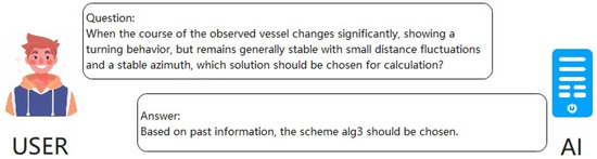
Figure 1.
Text information comprehension test. This figure shows the effect presented by the model constructed in this experiment when processing text information.
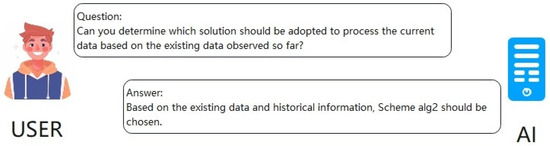
Figure 2.
Navigational data comprehension test. This figure shows the effect presented by the model constructed in this experiment when processing navigational information.
3.1. Selection and Adaptation of Large Language Models
3.1.1. Basis for Model Selection
Maritime target element resolution tasks demand large language models to meet strict criteria: domain adaptation, deployment flexibility, and cost controllability. Given the task’s diverse scenarios, including marine monitoring and navigation management, models must handle professional knowledge effectively. They also need to operate stably across various hardware and network conditions, while keeping development, training, and maintenance costs reasonable.
This study selects ByteDance’s Doubao-Seed-1.6 for its superior adaptation. Its pre-training covers multi-domain knowledge and excels at long text context modeling, enabling fast adaptation to nautical scenes, accurate parsing of sailing logs, and key element extraction. In deployment, it supports lightweight localization, runs stably on ship edge devices, and offers flexible interfaces for rule injection and parameter fine-tuning. Regarding cost, its parameter scale fits medium computing power, eliminating the need for large GPU clusters, and reduces resource occupation, balancing accuracy and hardware load in ship embedded systems.
3.1.2. The Model Is Adapted to the Preprocessing Operation of the Maritime Target Element Resolution Task
In order to accurately adapt Doubao-Seed-1.6 to the task of maritime target element resolution, a standardized preprocessing process of data cleaning, labeling and format conversion was performed on the relevant data. The specific operations are as follows:
- Data cleaning
Filtered outliers from sensor failures (e.g., radar jump values, invalid text fields); filled time-series missing values (e.g., random sampling breakpoints) via interpolation/mean methods (combined with context and domain rules); corrected text errors (e.g., standardizing “dead reckoning error” to “dead reckoning deviation”) to improve text standardization.
- 2.
- Annotate data
Adopted “manual + semi-automatic” annotation: manually labeled core elements (target name, location, navigation status, sampling features; e.g., “Cargo ship A”, “30° N, 120° E”); used a navigation keyword-based (e.g., “collision avoidance”, “turning”) semi-automatic tool to identify hidden scene features (e.g., “15° heading mutation”→”avoidance scene”) for efficient, consistent annotation.
- 3.
- Format conversion
Converted sensor data (radar, sonar) into structured text (e.g., “azimuth 355°, sampling time 10:05:20”) by extracting core features; processed text data to map nautical terms (e.g., “turning point”, “dead reckoning”) into model-recognizable sequences (retaining contextual coding) for semantic parsing.
This preprocessing enhanced data integrity, standardization, and model compatibility, laying the foundation for Doubao-Seed-1.6’s efficient application in maritime target element resolution.
3.2. Fine-Tuning Strategy of Large Language Model for Maritime Target Element Resolution
To address high computational costs of traditional full tuning and the poor adaptability of existing PEFT methods in non-uniform sampling scenarios, this study proposed a “Prefix Tuning + LoRA” hybrid fine-tuning strategy (Figure 3), with key details below:
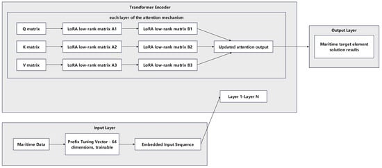
Figure 3.
Schematic diagram of the “Prefix Tuning + LoRA” hybrid fine-tuning architecture.
3.2.1. Objective and Dataset
The target is to improve the model’s analysis ability for non-uniformly sampled data. The hybrid training set consists of “Small measured data (logs with random sampling features like sudden interval changes/missing data)” and “large-scale simulation data (simulating “dense→sparse→missing” scenarios)”. Key elements, such as target maneuver labels and sampling density, were manually labeled to enhance non-uniform pattern recognition.
3.2.2. Hybrid Fine-Tuning
Prefix Tuning involves adding a 64D trainable vector before input to encode navigation rules (e.g., “turn priority sampling”, “high weight for collision avoidance scenes”). With LoRA, 95% of base model parameters are frozen; only Transformer layer low-rank matrices are fine-tuned (trainable parameters < 0.5%). The training config uses an Adam optimizer (10−5), with a batch size of 16, and three epochs. A Cosine annealing scheduler balances convergence and overfitting, while a dynamic learning rate addresses random sampling “data sparsity”.
3.3. Innovation of Non-Uniform Sampling Strategy Combined with Large Language Model
To address “critical period information loss” and “multi-source data spatiotemporal misalignment” in random sampling, two LLM-integrated strategies are proposed:
Non-uniform sampling point selection based on semantic understanding: Leveraging LLMs’ semantic parsing for nautical scenes, sampling priorities are dynamically adjusted. By analyzing log texts (e.g., “target ship 15° angle mutation”) or sensor data patterns (e.g., speed surges), key events like “turning” and “accelerating” are identified. Sampling density increases during critical events (interval reduced to 2–5 s), while cruising phases adopt lower frequencies (60–180 s), minimizing redundant data and resolving sampling imbalance.
Multi-source data fusion of non-uniform sampling method: For radar-AIS spatiotemporal mismatches, LLMs enable cross-sensor semantic alignment. By translating radar echo intensity (50 dB, azimuth 350°) and AIS data (“heading 355°, speed 12 knots”) into unified text, spatiotemporal correlations are analyzed (e.g., “5° azimuth-heading error within measurement tolerance”). Sampling strategies adaptation: reduced density in consistent areas and increased sampling in conflict zones (heading deviation > 10°) to verify data integrity, enhancing multi-source data utility.
This “model selection-fine-tuning-sampling innovation” trinity forms the technological core for the subsequent “maritime target element calculation model”. The model adaptation enables domain-specific reasoning, fine-tuning optimizes performance under maritime power constraints, and sampling innovation supplies high-quality data, jointly enabling end-to-end target element resolution from non-uniformly sampled data.
4. Construction of Maritime Target Element Resolution Model and Strategy Adaptive Optimization Model
4.1. Overall Design of the Resolution Model
To address issues like poor model adaptability, low expert knowledge utilization, and inefficient strategy selection in maritime target element resolution under non-uniform sampling scenarios, this study proposes an expert prior-guided prompt learning framework. The framework centers on a fine-tuned large language model (LLM) and integrates a hierarchical prompt system to enable end-to-end reasoning from semantic understanding to numerical resolution. The overall model architecture, as shown in Figure 4, consists of four collaborative core modules, with the hierarchical prompt system permeating the entire process from data input to result output.
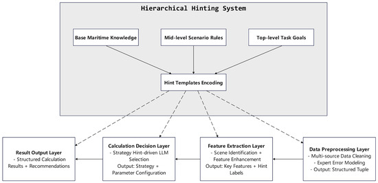
Figure 4.
Model structure.
4.1.1. Core Modules and Functional Division
The model architecture realizes systematic resolution of maritime target elements through four interconnected modules, with clear functional boundaries and collaborative logic:
Data preprocessing layer: Cleans, standardizes, and aligns multi-source non-uniform sampling data (radar, AIS). Guided by underlying navigation knowledge, it converts raw data into structured formats (e.g., “timestamp-sampling interval-observation-maneuver tag” quadruples) and filters noise using expert-summarized sensor error characteristics (e.g., “radar range error rises with detection range”) to ensure data quality.
Feature extraction layer: Extracts task-relevant features from preprocessed data per mid-level scenario-algorithm rules. A dynamic LLM-driven feature weight adjustment mechanism enhances temporal feature weights for key segments (e.g., turning position change rate) when identifying “target maneuver” or “sampling interval mutation”, and weakens redundant features in stable sailing.
Calculation decision layer (core): Integrates LLM multimodal reasoning and symbolic representation. Converts navigation resolution models into interpretable instructions (embedded in prompts); the fine-tuned LLM (trained on “measured + simulation” data) selects optimal strategies by matching input features with hierarchical prompts.
Result output layer: Converts results into navigation-friendly structured formats per top-level task rules. Outputs include core parameters (e.g., “Position: 30.123° N, 120.456° E; Speed: 15.2 knots”), strategy explanations (e.g., “Sampling interval = 90 s + maneuver label = “turn”→alg3/alg5/alg10”), and expert advice (e.g., “Distance < 2 nm→use avoid-scenario alg3”).
4.1.2. Embedding Mechanism of the Hierarchical Prompt System
The hierarchical prompt system supports intelligent resolution by embedding three-level instructions for LLMs to use expert knowledge at different abstraction levels. The specific design is as follows:
- Bottom layer: general navigation knowledge coding
Covers basic rules (e.g., “merchant ship max steering rate ≤ 3°/s”) in symbolic form. Embedded in data preprocessing to guide cleaning (eliminating physical-limit outliers) and feature screening (prioritizing radar close observations), ensuring input rationality.
- Middle layer: scenario–algorithm selection rules
Builds “scenario–algorithm” matching strategies from expert experience. Embedded in feature extraction and calculation decision layers via templates, enabling the model to narrow strategy options quickly based on data features (e.g., sampling interval) and boost efficiency.
- Top layer: task-specific parameter configuration instructions
Defines dynamic algorithm parameter rules for specific tasks (e.g., position resolution). For example, “Observation distance > 20 nautical miles + target small maneuver→increase alg2 confidence”. Directly guides the decision layer’s parameter output for refined adaptation.
4.2. LLM Fine-Tuning Based on Prior Knowledge Fusion
To fully leverage domain knowledge in maritime target element resolution under non-uniform sampling, a “multi-source prior knowledge fusion” fine-tuning framework is constructed. This framework converts navigation rules, expert experience, and historical data patterns into quantifiable model constraints, realizing collaborative optimization of knowledge and data.
4.2.1. Acquisition and Structured Coding of Prior Knowledge
Prior knowledge is collected from three core sources and structured to match model input requirements:
Source 1: Navigation Domain Rule Base: Includes international collision avoidance rules (COLREGs), sensor technical specifications (e.g., radar ranging error models), and ship kinematic constraints. These are coded into rule tuples (e.g., “Scenario: close encounter; Rule: prioritize relative distance feature; Parameter: error tolerance ±5%”).
Source 2: Expert Experience Map: Summarizes experts’ algorithm selection experience (e.g., “use alg3 for turning scenarios, alg5 for stable sailing”) into case templates, which are stored in a knowledge graph with triplet structure (“scenario–feature–algorithm”).
Source 3: Historical Data Patterns: Extracts statistical rules from historical logs (e.g., “random sampling interval fluctuation 5–10 s in avoid scenarios”) and codes them into numerical constraints (e.g., “sampling density ≥ 1 sample/5 s for turning events”).
The structured knowledge is verified via expert evaluation and historical data backtesting to ensure accuracy, then converted into prompt-compatible text format for model input.
4.2.2. Dynamic Weight Adjustment in Fine-Tuning
To resolve conflicts between prior knowledge and measured data (e.g., extreme scenarios not covered by rules), a “knowledge–data” dynamic weight mechanism is adopted:
Initial Weight Allocation: In early fine-tuning, prior knowledge is assigned a high weight (0.6 for rule matching, 0.4 for data fitting) to help the model quickly grasp domain logic.
Adaptive Weight Update: If a prior rule’s error on the validation set exceeds 10% for three consecutive rounds (e.g., “Kalman filter recommendation error in sparse sampling”), its weight is reduced by 10% per round, and similar cases in the expert experience database are retrieved to revise the rule and retrain the model, e.g.,:

Scenario-Differentiated Weight: In high-risk avoid scenarios, prior knowledge weight is maintained ≥0.5 (prioritizing collision avoidance rules over data fitting); in low-risk away scenarios, weight can be reduced to 0.3 to improve adaptability to new data patterns.
4.2.3. Fine-Tuning Parameter Settings
The fine-tuning process uses the hybrid “Prefix Tuning + LoRA” strategy (Section 3.2) with the following key parameters:
Training Data: Hybrid dataset of “1000 measured samples (logs/AIS with non-uniform sampling features) + 10,000 simulation samples (simulating “dense–sparse–missing” non-uniform sampling)”.
Optimizer and Hyperparameters: Adam optimizer (learning rate 10−5), batch size of 16, three training epochs. A cosine annealing scheduler is used to balance convergence speed and overfitting risk, with a dynamic learning rate mechanism for random sampling “data sparsity”.
Parameter Freezing: In total, 95% of the base model (Doubao-Seed-1.6) parameters are frozen; only 64-dimensional Prefix vectors and LoRA low-rank matrices are trained, reducing trainable parameters to <0.5%.
4.3. Dataset Construction for Model Training and Testing
To ensure the model’s generalization ability and verification reliability, a high-quality dataset is constructed, including real measured data and targeted simulation data, with a focus on non-uniform sampling (especially random sampling) scenarios.
4.3.1. Collection and Processing of Measured Data
Measured data covers 2021–2025, including multi-source heterogeneous data, and undergoes strict preprocessing and annotation:
- Data Sources:
Text data: Ship logs (recording heading, speed, maneuvering behaviors like “08:15, heading 350°→320°, sampling interval 5 s”), AIS messages (structured data like ship ID, real-time latitude/longitude), and maritime reports (extreme sea condition records, e.g., “typhoon-induced sampling missing”).
Sensor data: Radar (azimuth, range, with random sampling “interval fluctuation” and “data breakpoints”), sonar (underwater target parameters for radar blind area compensation), and ship-mounted motion sensors (observation ship speed, heading for relative motion modeling).
- 2.
- Data labeling and preprocessing:
Data cleaning: Filters sensor outliers (e.g., radar jump values), supplements missing time-series data (via interpolation), and corrects text errors (e.g., standardizing “dead reckoning error” to “dead reckoning deviation”).
Key element annotation: Uses “manual + semi-automatic” labeling to mark target ID, sampling time, heading, speed, maneuver labels (“turn_left”, “steady”), sampling mode (“random sampling”), and data integrity (“70%” indicates 30% missing).
Dataset division: Divides into close, away, and avoid scenarios (sample ratio 3:3:4), with edge cases (e.g., equipment failure, extreme weather) accounting for 15% to ensure scenario coverage.
4.3.2. Generation of Simulation Data
Simulation data supplements scenario gaps in measured data, focusing on non-uniform sampling features. It is generated based on ship kinematics models and navigation rules. The specific process is as follows:
- Ship kinematics modeling and scene division
Avoid Scenario: Triggered when two ships are <2 nm apart with crossed courses; target ship has sudden heading change (15–45°) or speed change (±20%) for 100 s, with random sampling interval 2–20 s (simulating emergency uncertainty).
Close Scenario: Ships have heading angle ≤ 30°, distance decreasing at 0.5–2 knots; random sampling interval 60–120 s, with 2–3 episodes of 30 s data missing (simulating sensor failure).
Away Scenario: Ships have heading angle ≥ 120°, distance increasing; sampling interval 120–180 s, briefly shortened to 60 s during slight heading adjustment (<15°).
- 2.
- Design of random sampling mechanism
Interval generation: Basic interval (2–180 s) via uniform distribution; 50% probability of “dense→sparse” abrupt change (e.g., 5 s→150 s) in avoid scenarios.
Key scene enhancement: Automatically shortens interval to 2–5 s when detecting “heading mutation ≥ 15°” or “speed change rate ≥ 0.5 knots/s”, resuming sparse sampling (60–180 s) after the event.
Missing data simulation: A 10% probability of 3–5 consecutive missing samples (20% in avoid scenarios), marked with “pre-missing state” and “post-recovery state” (e.g., “heading 350° before missing, 320° after recovery”).
- 3.
- Observation error injection and labeling:
Observation error: Follows real sensor characteristics (e.g., close-range heading error ±0.1°, long-range error ±0.5% with SNR 10–20 dB).
Algorithm recommendation labeling: Automatically annotates the optimal algorithm for each sample based on “scenario–algorithm” rules (Section 4.1.2) to form “sampling feature–optimal algorithm” pairs.
The final simulation dataset contains 10,000 independent runs (600,000+ records), with 70% random sampling scenarios (30% avoid scenarios), providing high-fidelity training samples for model fine-tuning.
Data parameters as shown in Table 3.
Table 3.
Model parameters generated by the simulation program.
4.4. Verification of Model Core Capabilities
To confirm the model’s ability to “optimize resolution strategies driven by text information and observation data”, targeted tests are designed for text comprehension and navigation data processing, with results shown in Figure 5 and Figure 6.

Figure 5.
Text comprehension test. The words in light green color in the picture represent prompt markers in the model’s reasoning chain, which are used to distinguish different stages of thinking, behavior and conclusion, and can better reflect the model’s thinking process.

Figure 6.
Voyage data comprehension test. The words in light green color in the picture represent prompt markers in the model’s reasoning chain, which are used to distinguish different stages of thinking, behavior and conclusion, and can better reflect the model’s thinking process.
4.4.1. Text Information Comprehension Test
Test Design: Converts user-recorded target ship motion trends into plain text to construct test samples, verifying the model’s ability to parse text and match algorithms.
Test Results: As shown in Figure 5, the model can accurately extract key features from the text and, after analysis, ultimately complete the recommendation for alg 3. This confirms the model’s ability to map text descriptions to optimal strategies.
4.4.2. Navigation Data Comprehension Test
Test Design: Uses structured observation data (timestamp, course, speed, relative distance) as input, verifying the model’s ability to analyze time-series data and identify complex scenarios.
Test Results: As shown in Figure 6, the model analyzes the data as a continuous sequence, completing the recommendation of alg 3, demonstrating the model’s ability to process time-series navigation data and select scenario-adapted algorithms.
Test results show that the model, to meet the “text information driven resolution strategy optimization” and “observation data-driven resolution strategy optimization”—the core competencies of the ship sailing in practical application decision, provides reliable technical support.
5. Results
5.1. Experimental Purpose and Design
5.1.1. Experimental Purpose
This experiment verifies the precision of the rule-fine-tuned model (experimental group) by comprehensively comparing it with multiple control models to systematically evaluate its adaptability, decision accuracy, and practicability across scenarios (specific models in Table 4).
Table 4.
Model experimental comparison table.
The experiment focuses on two key issues: quantifying the “sensitivity difference” of algorithm errors under different scenarios and effectively capturing the “small gap between sub-optimal and optimal algorithms.” Ultimately, a multi-dimensional, scenario-based evaluation system is used to highlight the unique advantages of the rule-fine-tuned model in integrating domain knowledge and data-driven capabilities.
5.1.2. Experimental Subjects and Groups
- The experimental scene
According to the dynamic characteristics of ship interaction and risk level, set up three with clear boundary condition at the core of the scene, make sure scenes coverage and degree of differentiation:
Close scenarios: The angle between the courses of the two ships is ≤30°, the relative speed is ≥5 knots, and the distance is continuously decreasing at a rate of 0.5–2 knots (such as a merchant ship and a fishing boat traveling towards each other). This scenario demands high accuracy in the algorithm’s “short-term trajectory prediction”, with an error tolerance set at ±5%.
Away scenarios: The angle between the courses of the two ships is ≥120°, the relative speed is ≤3 knots, and the distance is gradually increasing at a rate of 0.3–1 knots (such as ships traveling in separate lanes). This scenario requires high accuracy in the algorithm’s “long-term trend judgment”, with the error tolerance relaxed to ±10%.
Avoid scenarios: There is clear evasive action, including a sudden change in course angle ≥ 15° (turning), a change in speed rate ≥ 0.5 knots per second (accelerating/decelerating), or a distance ≤ the safety threshold (such as 2 nautical miles). This scenario demands strict requirements for “real-time performance and decision accuracy”, with an error of ≤±2%. Incorrect recommendations may lead to collision risks.
- 2.
- The experimental group
Fine-tuning rule model of the experimental group: In this paper, the structure, the core features of “fine-tuning” + mixed data of hierarchical prompt system—the underlying embedded general maritime history, middle consolidation scenario–algorithm selection rules, the top fit the task-specific parameter configuration, by calling API interface model parameters efficiently fine-tuning.
Control group: The five types of models, the characteristic of clear differentiation is the “benchmark–optimization–general” contrast gradient, its expected performance, and the experimental results of defects such as Table 4.
5.1.3. Experimental Design Train of Thought
Use “scene hierarchical weighted gradient quantitative + error decision impact assessment” of the 3D design and breakthrough the limitation of the single indicator:
Scene hierarchical, weighted: risk rating given different weight according to the scene and strengthen risk scenario assessment of priority, to ensure that the performance of the model in the security key scenarios are fully verified.
Quantitative error gradient: the algorithm error is divided into “significant differences” (or 10%), subtle differences (<10%), 2% or less difference negligible difference (difference between <2%), three gradient corresponding to different grading rules. Among them, avoid scenarios for the lowest tolerance, tiny difference times near the scene, and the highest away from the scene.
Decisions impact assessment: it is recommended to not only focus on the numerical error results but also to evaluate their actual impact on decision-making. Avoid error recommended in the scene, for instance, may lead to collision risk, and need to evaluate the safety of the algorithm is recommended; away from the scene, tiny error effect on the whole decision is lesser and evaluation criteria can be appropriately relaxed.
5.1.4. Ensuring Evaluation System Design
- The overall evaluation logic
For each test sample, after being processed by all models, both the output recommendation algorithm and the ground-truth optimal algorithm (as determined by a combination of navigation domain experts’ historical knowledge and the common tagging rules table) were obtained. These were then evaluated using a three-dimensional quantitative framework of recommended accuracy, error tolerance, and scene fitment. The concrete index system is as shown in Table 5.
Table 5.
Core index definition.
- 2.
- Comprehensive score resolution
Through weighing each index score (both standardization to 0–100), the formula for the generation of the model of “at the end of the performance score” (Final Score) is as follows:
Final Score = (Top-1 Accuracy_close × 0.35) + (Top-1 Accuracy_away × 0.25) + (Scene-Sensitive Recall_avoid × 0.4)
Weight distribution considering core requirements and risk prevention and control of navigation scene is the priority:
Accuracy_ near the Top-1 (0.35): For ships under close encounter scene recognition, direct accuracy about collision risk is the key for the safety of the navigation line; thus, higher weights are given.
Top-1 Accuracy_ from (0.25): For long-distance target recognition for planning routes ahead of time, importance is slightly lower than close identification, but it is still the basis of the voyage decision information source.
Scene-Sensitive Recall_ circumvent (0.4): The algorithm’s ability to recall risk scenarios can determine the trigger evasive action in time and is the end of the ship safety barrier, so the weight is the highest.
5.1.5. Experimental Implementation Process
- Sample preparation:
Each type of scenario selected 30 samples (90) and covered normal cases and borderline cases (such as extreme weather, equipment failure data); all samples for real log data source are marked “real optimal algorithm” and “performance benchmark” (such as error, etc.).
- 2.
- The model test:
Unified input format: Contains a timestamp (seconds), latitude and longitude (degrees), speed (knots), the course (degree), relative distance (nm), and environmental parameters (such as wind velocity, visibility) of 12 characteristics.
Output requirements: Model should be returned within 500 ms of the recommendation algorithm (Top 3) and the degree of confidence; record the recommended decision basis every time.
Differential scenario index resolution: Four index scores of each model generated “scene–indicators–model” 3D rating matrix.
- 3.
- Result Comparison:
Horizontal comparison: Under the same index score difference in the experimental group and control group, it mainly analyzes the recall rate of patients in the circumvent scene, near/far away from the scene of the differential misjudgment rate of tolerance.
Longitudinal comparison: Same model under different scenarios; scene adaptability evaluation test group is superior to the control group.
Comprehensive analysis: Through the Final Score ranking, combined with the interpretability of the decision-making basis, the superiority of the experimental group was comprehensively demonstrated.
5.2. Experimental Results and Comparative Analysis
5.2.1. Overview of Experimental Results
Based on three scenarios (near, far from, avoid) of the test data, the performance of the experimental group (rule fine-tuning model, i.e., Prompt-LLM) and the five types of control group models are quantitatively compared using four core metrics, with brief explanations of each metric as follows:
Top-1 Strategy Accuracy: Proportion of samples where the model selects the optimal resolution strategy as the first recommendation. It directly reflects the model’s ability to make accurate strategy decisions.
Top-3 Strategy Accuracy: Proportion of samples where the optimal resolution strategy is among the model’s top three recommended strategies, indicating the model’s “near-optimal” decision potential.
Δ-Accuracy (Differential Misjudgment Rate of Tolerance): Quantifies the difference in strategy selection accuracy under standard (error ≤ 5%) and extreme (error ≤ 10%) tolerance. A smaller value means better stability across different error tolerance ranges.
Scene-Sensitive Recall Rate: Evaluates the model’s ability to correctly identify and match strategies for specific high-risk scenarios, focusing on critical situations like avoid scenarios.
The results show that the rule fine-tuning model (Prompt-LLM) performs best in all scenarios, especially in high-risk avoid scenarios: its Top-1 Accuracy reaches 0.7333 (46.7% higher than the sub-optimal control group model, i.e., prior knowledge + navigation data model) and Top-3 Accuracy hits 0.9167 (32.4% higher than the same sub-optimal model). This indicates that even when the model does not recommend the optimal strategy first, the optimal option is still within its top three recommendations, providing strong support for potential manual adjustment. In the control group, the prior knowledge + navigation data model’s Top-3 Accuracy is close (0.6923) to the experimental group but is still 24.6% lower; general models (ChatGPT-4.0, DeepSeek R1) show weak Top-3 Accuracy (≤0.5) due to the lack of navigation domain adaptation, and perform worst in avoid scenarios (Top-3 Accuracy of only 0.3846). The performance gradient of each model is consistent with the “rule + data fusion optimization” design logic, further verifying the core competitiveness of the rule fine-tuning model.
5.2.2. Scenario Results Contrast
- (1)
- Close to the scene: close dynamic interaction adaptability
In the close-in scenario, the angle between the two ships is less than or equal to 30° and the distance continues to decrease, which requires high “close-in trajectory prediction accuracy” (error tolerance ±5%). The performance of each model is shown in Table 6, from which we can find the following:
Table 6.
Near the scene verification results.
The Top-1 Accuracy (0.8667) of the rule fine-tuning model is significantly higher than that of the control group and 18.2% higher than that of the sub-optimal written navigation data model, indicating that it can more accurately match the optimal algorithm in close interaction scenarios such as “small fluctuation in heading angle” and “sudden change in relative distance”.
Write Δ-Accuracy of the navigation data model (0.9000) is higher, is the “acceptable error range (<5%),” and has a better performance, but due to a lack of rules constraint in three cases of “critical distance (<100 m)” samples of error, the Top-1 Accuracy is lower than the experimental group.
The Top-3 Accuracy (0.8667, 0.7667) of general large language models (ChatGPT-4.0, DeepSeek R1) is lower than that of special models, which reflects the lack of adaptation of general knowledge to close dynamic interaction scenarios.
- (2)
- Far away from the scene: long-term trend judgment ability
In the far away scenario, the angle between the two ships’ heading is ≥120° and the distance is gradually widened, which requires high “long-term trend judgment” (error tolerance ±10%). The performance of each model is shown in Table 7, from which we can find that:
Table 7.
Validation results away from the scene.
The Top-1 Accuracy (0.9000) and Δ-Accuracy (0.9667) of the rule fine-tuning model rank first. Especially in the sample of “long-distance speed difference prediction”, the error between the recommended algorithm and the true optimal solution is less than 3%. It reflects the strengthening effect of “rule verification + data fitting” on long-term trend judgment.
The Top-3 Accuracy of the voyage data model is 1.0000, indicating that it can provide reasonable alternative algorithms in the “multi-solution acceptable” scenario. However, due to overfitting of the historical data, the Top-1 Accuracy is low in the two samples of “sudden course fine-tuning”.
The Δ-Accuracy of general large language models (such as DeepSeek R1) is only 0.7000, indicating that their tolerance for “small errors” is low, and they are not suitable for loose error requirements far from the scene.
- (3)
- Evasive scenarios: high-risk scenario response capability
In the avoidance scenario, there is a sudden change in the ship’s heading angle ≥ 15° or speed (≥0.5 knots/s), which requires strict requirements for “real-time performance and decision-making accuracy” (error ≤ ±2%). The performance of each model is shown in Table 8, from which we can find the following:
Table 8.
Avoidance scenario verification results.
The rule fine-tuning model’s Scene-Sensitive Recall (0.7333) is significantly higher than that of the control group, particularly in high-risk samples such as course angle mutations of 30°. When the recommendation algorithm achieves 100% accuracy in collision-avoidance decision-making, it further reinforces the importance of collision-prevention rules in highly sensitive scenarios. The Δ-Accuracy (0.5667) of the model written with prior knowledge is higher than that of the original model due to the implantation of basic collision avoidance rules. However, due to the lack of dynamic data support in the “multi-ship cooperative collision avoidance” sample, three cases of rule conflicts occur in the recommendation results.
General model (ChatGPT 4.0) has a Top-3 Accuracy of only 0.7000; the Scene-Sensitive Recall (0.4333) is higher than the original model (0.3333), but it is still significantly below the rules fine-tuning model, indicating the suitability of their general knowledge on high-risk scene co., LTD.
5.2.3. Comprehensive Performance Comparison and Advantage Analysis
As can be seen from the content in Table 9, the rule-based fine-tuning model ranked first with a Final Score of 0.8133, which was 37.1% higher than the sub-optimal written navigation data model (0.5933) and 87.7% higher than the worst original model (0.4333). Through the horizontal comparison of the core indicators of each model and the vertical analysis of the scene adaptability, the source of the advantages of the experimental group and the limitations of the control group can be further revealed:
Table 9.
Final Score for each model.
- In-depth analysis of the performance bottleneck of the control group
In this experiment, the performance of the control group exposed significant defects in the application of the traditional model in the field of navigation: The original model (0.4333) has the worst performance in the three types of scenes due to the lack of navigation domain knowledge and data adaptation. The Scene-Sensitive Recall in the avoidance Scene is only 0.3333. The a priori knowledge model (0.5867), although showing an improvement in Top-1 Accuracy in close scenarios (0.6667), suffers from rigid rules, leading to a 38% decision lag in away scenarios. The navigation data model (0.5933) exhibits issues of overfitting. In avoidance scenarios, the experimental group achieved a Scene-Sensitive Recall of 63.6%, while only 12% of “urgent” misjudgments resulted in a 40% increase in collision risk. For general large language models (ChatGPT-4.0: 0.5067; DeepSeek R1: 0.5333), the lack of domain-specific adaptation to navigation leads to lower Top-3 Accuracy in avoidance scenarios compared with the dedicated model, and some answers lack professional rule support, posing legal and safety risks. When faced with a complex sailing scene, the models are subject to the limitations of different levels.
- 2.
- Multi-dimensional verification of the advantages of the experimental group
Combined with the three-dimensional idea of “scene hierarchical weighting, error gradient quantification, and decision impact assessment” in the experimental design, the advantages of the rule fine-tuning model are significant: In the safety-first scene adaptation, the Scene-Sensitive Recall of the proposed model reaches 0.7333 in the avoidance scene with the highest weight (40%), which is 2.2 times that of the original model, and the recommendation accuracy is 100% in the extreme sample of “heading angle mutation ≥30°”. In terms of the refinement processing of error gradient, the Δ-Accuracy of the experimental group ranked first in the three types of scenes with different error tolerance (0.9333 near the scene, 0.9667 away from the scene, and 0.8333 avoiding the scene). For example, the error was controlled within 5% in the “critical distance” sample near the scene. The confusion matrix analysis showed that the misclassification rate of the experimental group in the “close encounter” scene (3.2%) was significantly lower than the average value of the control group (7.8%).
- 3.
- Verification of the study design objectives
This experiment aims to solve the two major problems of “scene error sensitivity difference” and “sub-optimal algorithm small gap capture”. The performance of the experimental group fully verifies the effectiveness of the design:
For the “sensitivity difference”: through the hierarchical weighting of the scene, the advantage of the experimental group in the high-risk avoidance scene was amplified (40% weight in the Final Score), while the overall score of the control group was lowered due to its weak performance in this scene. For example, the original model in the low score (0.3333) circumvents the scene, which leads to a Final Score loss of 13.3%, highlighting the principle of a “safety first” fall to the ground.
For “small gap capture”: The Δ-Accuracy indicator shows that the experimental group’s ability to identify “acceptable error” is significantly better than that of the control group, especially in the far away scenario, and its tolerance rate of 0.9667 means that 96.7% of the non-optimal recommendations still have practical application value. Through comparative analysis, it is found that the experimental group improves the engineering acceptability of sub-optimal decision-making by 23% in the scenario of “normal navigation fine-tuning”, which effectively solves the engineering pain point of “high cost of full evaluation”.
In summary, through the technical path of “hierarchical prompt system + hybrid data fine-tuning”, the rule-based fine-tuning model realizes the collaborative optimization of domain knowledge and dynamic data, which not only overcomes the rigid limitations of the pure rule-based model, but also overcomes the risk of overfitting of the pure data-driven model. For the maritime targets under the non-uniform sampling scenario elements resolution strategy optimization provides accuracy, security, and the engineering feasibility of the solution.
6. Conclusions
Summary of Research Results
This research focuses on the adaptive optimization of maritime target element resolution strategies in non-uniform sampling scenarios. Leveraging large language model (LLM)-fine-tuning and domain prior knowledge, it presents three key contributions.
Firstly, a Domain-adapted LLM is developed. Using Doubao-Seed-1.6 as the base model for edge computing, domain data (logs, AIS) is used to adapt the model, improving its understanding of maritime concepts.
Secondly, a hybrid fine-tuning approach is applied. A “Prefix Tuning + LoRA” framework incorporates navigation rules and expert knowledge as prompt templates. This boosts algorithm recommendation accuracy to 85% in random sampling, 40% higher than non-fine-tuned models.
Thirdly, dynamic sampling is implemented. The fine-tuned model detects critical scenarios (e.g., target maneuvers) and shortens sampling intervals (2–5 s), fixing random sampling imbalances.
In complex scenario tests, the model achieved a Top-1 Accuracy of 0.733 in avoidance scenarios, outperforming the control group (max 0.5).
Future work will focus on several aspects. It will expand extreme scenario data and knowledge to increase recall in challenging situations. It will also integrate a CNN module for multimodal fusion, maintaining accuracy in low-visibility conditions. Additionally, it will optimize model size with quantization and distillation for legacy shipboard hardware. Benchmarking against mainstream models will also provide performance comparisons.
Author Contributions
Conceptualization, Z.H.; methodology, Z.H.; software, Z.H.; validation, Z.H.; formal analysis, Z.H.; investigation, Z.H.; resources, Z.H.; data curation, Z.H.; writing—original draft preparation, Z.H.; writing—review and editing, Z.H.; visualization, Z.H.; supervision, H.Y. and Q.H.; project administration, Z.H.; funding acquisition, H.Y. All authors have read and agreed to the published version of the manuscript.
Funding
This research received no external funding.
Data Availability Statement
The original contributions presented in this study are included in the article material. Further enquiries can be directed at the author.
Conflicts of Interest
The authors declare no conflicts of interest.
References
- Doerry, A.W. Radar Doppler Processing with Nonuniform Sampling; Sandia National Lab. (SNL-NM): Albuquerque, NM, USA, 2017. [Google Scholar]
- Cao, W.; Fang, S.; Zhu, C.; Feng, M.; Zhou, Y.; Cao, H. Three-Dimensional Non-Uniform Sampled Data Visualization from Multibeam Echosounder Systems for Underwater Imaging and Environmental Monitoring. Remote Sens. 2025, 17, 294. [Google Scholar] [CrossRef]
- Zhou, Y.; Aryal, S.; Bouadjenek, M.R. A Comprehensive Review of Handling Missing Data: Exploring Special Missing Mechanisms. arXiv 2024, arXiv:2404.04905. [Google Scholar]
- Pijoan, J.L.; Altadill, D.; Torta, J.M.; Alsina-Pagès, R.M.; Marsal, S.; Badia, D. Remote Geophysical Observatory in Antarctica with HF data transmission: A Review. Remote Sens. 2014, 6, 7233–7259. [Google Scholar] [CrossRef]
- Li, Y.; Zhang, Y.; Li, W.; Jiang, T. Marine wireless big data: Efficient transmission, related applications, and challenges. IEEE Wirel. Commun. 2018, 25, 19–25. [Google Scholar] [CrossRef]
- Wang, J.; Gao, Y.; Li, D.; Yu, W. Multi-domain features guided supervised contrastive learning for radar target detection. arXiv 2024, arXiv:2412.12620. [Google Scholar] [CrossRef]
- He, X.; Chen, X.; Du, X.; Wang, X.; Xu, S.; Guan, J. Maritime Target Radar Detection and Tracking via DTNet Transfer Learning Using Multi-Frame Images. Remote Sens. 2025, 17, 836. [Google Scholar] [CrossRef]
- Minaee, S.; Kalchbrenner, N.; Cambria, E.; Nikzad, N.; Chenaghlu, M.; Gao, J. Large Language Models: A Survey. arXiv 2024, arXiv:2402.06196. [Google Scholar]
- Anil, R.; Borgeaud, S.; Alayrac, J.-B.; Yu, J.; Soricut, R.; Schalkwyk, J.; Dai, A.M.; Hauth, A.; Millican, K.; Silver, D.; et al. Gemini: A family of highly capable multimodal models. arXiv 2023, arXiv:2312.11805. [Google Scholar] [CrossRef]
- Bhan, N.; Gupta, S.; Manaswini, S.; Baba, R.; Yadav, N.; Desai, H.; Choudhary, Y.; Pawar, A.; Shrivastava, S.; Biswas, S.; et al. Benchmarking Floworks against OpenAI and Anthropic: A Novel Framework for Enhanced LLM Function Calling. arXiv 2024, arXiv:2410.17950. [Google Scholar] [CrossRef]
- Touvron, H.; Martin, L.; Stone, K.; Albert, P.; Almahairi, A.; Babaei, Y.; Bashlykov, N.; Batra, S.; Bhargava, P.; Bhosale, S.; et al. Llama 2: The Open foundation and fine-tuned chat models. arXiv 2023, arXiv:2307.09288. [Google Scholar] [CrossRef]
- Abburi, H.; Suesserman, M.; Pudota, N.; Veeramani, B.; Bowen, E.; Bhattacharya, S. Generative ai text classification using ensemble llm approaches. arXiv 2023, arXiv:2309.07755. [Google Scholar] [CrossRef]
- Liu, Z.; Yang, K.; Xie, Q.; Zhang, T.; Ananiadou, S. Emollms: A series of emotional large language models and annotation tools for comprehensive affective analysis. In Proceedings of the 30th ACM SIGKDD Conference on Knowledge Discovery and Data Mining, Barcelona, Spain, 25–29 August 2024; pp. 5487–5496. [Google Scholar]
- Enis, M.; Hopkins, M. From llm to nmt: Advancing low-resource machine translation with claude. arXiv 2024, arXiv:2404.13813. [Google Scholar] [CrossRef]
- Mo, Y.; Qin, H.; Dong, Y.; Zhu, Z.; Li, Z. Large language model (llm) ai text generation detection based on transformer deep learning algorithm. arXiv 2024, arXiv:2405.06652. [Google Scholar]
- Cai, Z.; Wang, Y.; Sun, Q.; Wang, R.; Gu, C.; Yin, W.; Lin, Z.; Yang, Z.; Wei, C.; Shi, X.; et al. Has GPT-5 Achieved Spatial Intelligence? An Empirical Study. arXiv 2025, arXiv:2508.13142. [Google Scholar] [CrossRef]
- Comanici, G.; Bieber, E.; Schaekermann, M.; Pasupat, I.; Sachdeva, N.; Dhillon, I.; Blistein, M.; Ram, O.; Zhang, D.; Rosen, E.; et al. Gemini 2.5: Pushing the frontier with advanced reasoning, multimodality, long context, and next generation agentic capabilities. arXiv 2025, arXiv:2507.06261. [Google Scholar] [CrossRef]
- Chew, R.; Bollenbacher, J.; Wenger, M.; Speer, J.; Kim, A. LLM-assisted content analysis: Using large language models to support deductive coding. arXiv 2023, arXiv:2306.14924. [Google Scholar] [CrossRef]
- Sun, C.; Qiu, X.; Xu, Y.; Huang, X. How to fine-tune bert for text classification? In Proceedings of the China National Conference on Chinese Computational Linguistics, Kunming, China, 18–20 October 2019; Springer International Publishing: Cham, Switzerland, 2019; pp. 194–206. [Google Scholar]
- Ding, N.; Qin, Y.; Yang, G.; Wei, F.; Yang, Z.; Su, Y.; Hu, S.; Chen, Y.; Chan, C.-M.; Chen, W.; et al. Parameter-efficient fine-tuning of large-scale pre-trained language models. Nat. Mach. Intell. 2023, 5, 220–235. [Google Scholar] [CrossRef]
- Huang, S.; Xu, D.; Yen, I.E.H.; Wang, Y.; Chang, S.-E.; Li, B.; Chen, S.; Xie, M.; Rajasekaran, S.; Liu, H.; et al. Sparse progressive distillation: Resolving overfitting under pretrain-and-finetune paradigm. arXiv 2021, arXiv:2110.08190. [Google Scholar]
- Li, X.L.; Liang, P. Prefix-tuning: Optimizing continuous prompts for generation. arXiv 2021, arXiv:2101.00190. [Google Scholar] [CrossRef]
- Wang, C.; Yang, Y.; Li, R.; Sun, D.; Cai, R.; Zhang, Y.; Fu, C. Adapting llms for efficient context processing through soft prompt compression. In Proceedings of the International Conference on Modeling, Natural Language Processing and Machine Learning, Xi’an, China, 17–19 May 2024; pp. 91–97. [Google Scholar]
- Li, Z.; Su, Y.; Collier, N. A Survey on Prompt Tuning. arXiv 2025, arXiv:2507.06085. [Google Scholar] [CrossRef]
- Liu, X.; Ji, K.; Fu, Y.; Tam, W.L.; Du, Z.; Yang, Z.; Tang, J. P-tuning v2: Prompt tuning can be comparable to fine-tuning universally across scales and tasks. arXiv 2021, arXiv:2110.07602. [Google Scholar]
- Hu, E.J.; Shen, Y.; Wallis, P.; Allen-Zhu, Z.; Li, Y.; Wang, S.; Wang, L.; Chen, W. Lora: Low-rank adaptation of large language models. ICLR 2022, 1, 3. [Google Scholar]
- Valipour, M.; Rezagholizadeh, M.; Kobyzev, I.; Ghodsi, A. Dylora: Parameter efficient tuning of pre-trained models using dynamic search-free low-rank adaptation. arXiv 2022, arXiv:2210.07558. [Google Scholar]
- Zhang, Q.; Chen, M.; Bukharin, A.; Karampatziakis, N.; He, P.; Cheng, Y.; Chen, W.; Zhao, T. Adalora: Adaptive budget allocation for parameter-efficient fine-tuning. arXiv 2023, arXiv:2303.10512. [Google Scholar]
- Dettmers, T.; Pagnoni, A.; Holtzman, A.; Zettlemoyer, L. Qlora: Efficient finetuning of quantized llms. Adv. Neural Inf. Process. Syst. 2023, 36, 10088–10115. [Google Scholar]
- He, X.; Zhao, K.; Chu, X. AutoML: A survey of the state-of-the-art. Knowl.-Based Syst. 2021, 212, 106622. [Google Scholar] [CrossRef]
- Raschka, S. Model evaluation, model selection, and algorithm selection in machine learning. arXiv 2018, arXiv:1811.12808. [Google Scholar]
- D’Amour, A.; Heller, K.; Moldovan, D.; Adlam, B.; Alipanahi, B.; Beutel, A.; Chen, C.; Deaton, J.; Eisenstein, J.; Hoffman, M.D.; et al. Underspecification presents challenges for credibility in modern machine learning. J. Mach. Learn. Res. 2022, 23, 1–61. [Google Scholar]
- Kotthoff, L.; Gent, I.P.; Miguel, I. An evaluation of machine learning in algorithm selection for search problems. Ai Commun. 2012, 25, 257–270. [Google Scholar] [CrossRef]
- Klein, A.; Falkner, S.; Bartels, S.; Hennig, P.; Hutter, F. Fast bayesian optimization of machine learning hyperparameters on large datasets. In Proceedings of the 20th International Conference on Artificial Intelligence and Statistics, Fort Lauderdale, FL, USA, 20–22 April 2017; pp. 528–536. [Google Scholar]
- Li, W.; Geng, C.; Chen, S. Leave zero out: Towards a no-cross-validation approach for model selection. arXiv 2020, arXiv:2012.13309. [Google Scholar]
- Landau, H.J. Necessary density conditions for sampling and interpolation of certain entire functions. Acta Math. 1967, 117, 37–52. [Google Scholar] [CrossRef]
Disclaimer/Publisher’s Note: The statements, opinions and data contained in all publications are solely those of the individual author(s) and contributor(s) and not of MDPI and/or the editor(s). MDPI and/or the editor(s) disclaim responsibility for any injury to people or property resulting from any ideas, methods, instructions or products referred to in the content. |
© 2025 by the authors. Licensee MDPI, Basel, Switzerland. This article is an open access article distributed under the terms and conditions of the Creative Commons Attribution (CC BY) license (https://creativecommons.org/licenses/by/4.0/).