Abstract
An adaptive sliding mode controller (SMC) design with a reinforcement-learning parameter optimization method is proposed for variable-speed trajectory tracking control of underactuated vessels under scenarios involving model uncertainties and external environmental disturbances. First, considering the flexible control requirements of the vessel’s propulsion system, the desired navigation speed is designed to satisfy an S-curve acceleration and deceleration process. The rate of change of the trajectory parameters is derived. Second, to address the model uncertainties and external disturbances, an extended state observer (ESO) is designed to estimate the unknown bounded disturbances and to provide feedforward compensation. Moreover, an adaptive law is designed to estimate the upper bound of the unknown disturbances, ensuring system stability even in the presence of asymptotic observation errors. Finally, the Twin-Delayed Deep Deterministic Policy Gradient (TD3) algorithm is employed for real-time controller parameter tuning. Numerical simulation results demonstrate that the proposed method significantly improves the trajectory tracking accuracy and dynamic response speed of the underactuated vessel. Specifically, for a sinusoidal trajectory with an amplitude of 200 m and a frequency of 0.01, numerical results show that the proposed method achieves convergence of the longitudinal tracking error to zero, while the lateral tracking error remains stable within 1 m. For the circular trajectory with a radius of 300 m, the numerical results indicate that both the longitudinal and lateral tracking errors are stabilized within 1 m. Compared with the fixed-value sliding mode controller, the proposed method demonstrates superior trajectory tracking accuracy and smoother control performance.
1. Introduction
Driven by the significant advancements in artificial intelligence (AI) and machine learning (ML) technologies, underactuated vessels have shown considerable potential in applications such as marine surveying, hydro-meteorological observation, and transportation [1]. Compared with traditional fully actuated vessels, underactuated vessels are gaining attention due to their simplified structure, reduced energy consumption, and cost advantages. However, the reduction in the number of actuators (propellers or rudders) results in a decrease in the system’s controllable degrees of freedom (DOF), which makes motion control in complex marine environments more challenging. The motion control of underactuated vessels primarily includes trajectory tracking, dynamic positioning, and automatic berthing. Typically, these control methods are implemented on embedded system platforms; for example, the Robot Operating System (ROS). By executing control algorithms in real time on an embedded controller, both a fast response and high-precision control should be satisfied. Furthermore, the compact size and low power consumption of embedded devices provide optimal hardware support for the deployment of vessel control systems. With the rapid development and application of unmanned vessels, trajectory tracking control has become critical for enhancing the safety and efficiency of unmanned vessel operations in marine environments. Trajectory tracking requires the vessel to precisely follow a predetermined path and to reach the target position within the specified time frame. In practice, the vessel must adjust its rudder torque and propeller thrust to correct its position and heading in real time, compensating for deviations between the desired trajectory and actual trajectory caused by external disturbances such as wind, waves, and currents. Due to the nonlinear characteristics, large inertia effects, and model uncertainties of the underactuated vessel, the development of robust trajectory tracking control algorithms with a fast response, high accuracy, and effective disturbance rejection has become crucial for solving the motion control problems of underactuated vessels.
Many scholars have conducted studies on the control of trajectory tracking. Classical linear control methods, such as PID controllers [2,3,4,5,6] and the Linear Quadratic Regulator (LQR) [7,8,9,10], have proven effective in enhancing the tracking accuracy as well as in improving system stability and robustness. However, these methods exhibit limited adaptability for complex systems and typically rely on precise system models. In contrast, SMC exhibits superior robustness and adaptability in environments with severe nonlinearities and high disturbances [11,12,13,14,15]. Consequently, SMC has become an effective approach for achieving precise control of trajectory tracking.
Despite the numerous advantages of SMC, it also has certain limitations. For instance, high-frequency switching inherent in SMC can lead to sharp fluctuations in the control signal, which may negatively impact the actuators. Additionally, designing an appropriate sliding surface for complex systems often requires substantial theoretical and empirical foundations. Moreover, when the system state has not yet reached the sliding surface, the initial performance of SMC may be suboptimal, leading to less effective control. To address these challenges, extensive research has been dedicated to enhancing the performance and expanding the applicability of SMC. Mao et al. [16] addressed the challenges of input distribution uncertainty and system uncertainties in nonlinear systems by designing an observer to estimate and compensate for these uncertainties. They proposed an adaptive SMC to achieve stable control of nonlinear systems. Zhou et al. [17] focused on second-order nonlinear systems and designed a periodic delayed sliding mode surface, introducing a non-singular SMC to ensure that the system states converge to zero within a predetermined time. Wang et al. [18] tackled issues related to switching mechanisms, nonlinearity, and uncertainties in systems by proposing a switching fuzzy integral sliding mode surface. The effectiveness of this approach was demonstrated through theoretical analysis and numerical validation. Gandikota et al. [19] addressed nonlinearities and model mismatches by integrating adaptive mechanisms with super-twisting SMC, thereby enhancing system robustness and tracking performance. Numerous researchers have made significant improvements to SMC in complex nonlinear environments, leading to their widespread application in various engineering problems [20,21]. Similarly, SMC has also gained broad recognition in the field of vessel trajectory tracking control. Herman [22] addressed the trajectory tracking control problem for underactuated marine vehicles by designing a first-order integral sliding mode surface combined with a constant-speed reaching law. He proposed an adaptive integral SMC, achieving trajectory tracking for vehicles with symmetric inertia matrices. Zhu et al. [23] developed an exponential terminal SMC for underactuated unmanned surface vessels (USVs). Simulation results demonstrated that compared with a global integral SMC, the proposed exponential SMC exhibited superior convergence and robustness. Wang et al. [24] focused on the trajectory tracking problem in the horizontal plane of underactuated autonomous underwater vehicles (AUVs) and proposed a non-singular fast terminal SMC incorporating an exponential reaching law, which improved tracking speed and was validated through simulations. Xu et al. [25] introduced a non-singular terminal SMC for underactuated USVs. They designed a nonlinear ESO to estimate complex environmental disturbances, effectively addressing input saturation and enabling trajectory tracking control under unknown external disturbances. Wu et al. [26] proposed a dual-loop control structure for the three-dimensional trajectory tracking of underactuated AUVs. The inner-loop controller, based on non-singular integral terminal SMC, ensured rapid trajectory tracking and finite-time convergence. Lei et al. [27] presented an adaptive fast non-singular terminal SMC for underactuated vessel trajectory tracking, accelerating error convergence and avoiding singularity issues. They employed the dynamic surface control method to address the “differentiation explosion” problem, used an adaptive law to estimate the upper bound of unknown disturbances, and mitigated chattering by substituting the conventional sign function with a hyperbolic tangent function. Sun et al. [28] designed a dual-loop control system for trajectory tracking of underactuated USVs equipped with vector propulsion systems. They introduced a non-singular integral terminal SMC approach and approximated unknown disturbances using the minimal learning parameter theory, achieving precise control of the USVs. Zhang et al. [29] addressed finite-time trajectory tracking control for surface vessels affected by dynamic uncertainties and unknown time-varying disturbances. They used adaptive neural networks to approximate dynamic uncertainties and estimated error bounds through adaptive laws. Zhang et al. [30] tackled the trajectory tracking control problem for underactuated autonomous surface vessels subject to dynamic uncertainties and nonlinear external disturbances. They employed neural networks and low-frequency learning techniques to estimate and approximate system uncertainties effectively.
In summary, various improvements have been proposed by scholars to mitigate the chattering problem in SMC. These include the use of saturation functions, exponential approaching laws, and second-order sliding mode control, which effectively reduce the impact on actuators by smoothing the switching process. In terms of the sliding surface design, researchers typically combine Lyapunov stability theory with practical engineering experience to optimize the parameter settings of the sliding surface, thereby adapting it to the dynamic characteristics of different systems. Moreover, to enhance the performance of SMC during the initial approaching phase, some studies have integrated SMC with other control methods, such as adaptive control, fuzzy control, or deep reinforcement-learning algorithms. These hybrid control strategies significantly improve the response performance of SMC in complex environments. Therefore, this paper proposes a TD3-tuned SMC integrated with an ESO to estimate and feedforward compensate for unknown disturbances. Furthermore, existing research has mostly focused on constant-speed trajectory tracking. However, in practical vessel motion, the vessel’s speed often undergoes significant variations, especially during the automatic berthing process, where the speed changes are particularly pronounced. Endo [31] designed a corresponding berthing controller based on the typical steps of berthing (e.g., “full speed—half speed—slow speed—stop”) and established the relationship between vessel speed and propeller speed through a questionnaire survey. This approach was successfully applied in the controller design. In this context, this paper proposes a variable-speed trajectory tracking controller that meets the maneuvering requirements for port entry and exit, with the desired speed designed to follow an S-curve acceleration/deceleration profile.
This paper investigates the variable-speed trajectory tracking control problem for underactuated vessels, with the following main contributions: (1) In response to the maneuvering requirements during port entry and exit, a desired speed profile based on an S-curve acceleration/deceleration process is designed, and a variable-speed trajectory tracking controller is developed to address practical requirements; (2) An ESO is designed to estimate and compensate for unknown disturbances via feedforward control, and global system stability is analyzed using Lyapunov functions; (3) The TD3 algorithm is proposed to optimize the SMC parameters. By employing multiple networks and selecting the minimum value, the issue of value overestimation in reinforcement learning is addressed. Additionally, the delayed update strategy improves the stability of the actuator network, resulting in smoother parameter outputs from the SMC.
The remainder of this paper is organized as follows. Section 2 establishes a 3-DOF vessel model and defines the trajectory tracking problem. Section 3 utilizes an ESO to estimate and compensate for unknown disturbances through feedforward control and designs a SMC with TD3 algorithm optimization. Section 4 introduces the overall structure of the control system. Section 5 validates the effectiveness of the proposed algorithm through simulation results. Finally, Section 6 presents the conclusions.
2. Problem Formulation and Preliminaries
2.1. Problem Formulation
Before designing the trajectory tracking controller, this paper establishes an underactuated vessel’s 3-DOF control model. The model considers surge, sway, and yaw motions, providing the foundation for the subsequent control system design. The body-fixed coordinate system {b} and the inertial coordinate system {n} are shown in Figure 1, denoted as and , respectively. The body-fixed coordinate system {b} typically has its origin at the vessel’s center of gravity, with pointing along the vessel’s heading direction on the horizontal plane, pointing to the vessel’s starboard side, perpendicular to the vessel’s longitudinal profile, and pointing vertically upwards. The inertial coordinate system {n} typically has its origin at the earth’s center, with pointing toward the north, pointing toward the east, and pointing toward the center of the Earth. The vessel’s control model is then given by Equations (1) and (2):
Here, , , and denote the longitudinal linear velocity, lateral linear velocity, and yaw angular velocity, respectively, of the vessel in the {b} coordinate system. , , and denote the longitudinal coordinate, lateral coordinate, and yaw angle, respectively, of the vessel in the {n} coordinate system. and denote the longitudinal thrust from the vessel’s propeller and the rudder torque in the {b} coordinate system, respectively. , , and denote the longitudinal interference force, lateral interference force, and yaw interference moment, respectively, acting on the vessel in the {b} coordinate system. , , and denote the respective viscous forces acting on the vessel due to the fluid in the {b} coordinate system. , , and denote the total mass of the vessel, including the additional mass and inertia generated by the fluid’s inertial forces, respectively. Equation (1) denotes the kinematic model of the vessel, describing the relationship between the body-fixed coordinate system {b} and the inertial coordinate system {n}. Equation (2) denotes the dynamic model of the vessel, describing the forces acting on the vessel in the body-fixed coordinate system {b}.
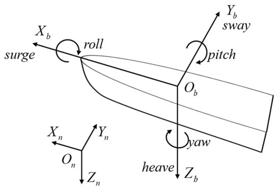
Figure 1.
The inertial coordinate system and the ship body coordinate system.
Typically, underactuated vessels often use podded propulsion systems as their power devices. The forces generated by the pod system primarily consist of the propeller thrust and the lateral force , and their calculation formulas are given by Equation (3):
Here, denotes the seawater density. denotes the propeller rotational speed. denotes the propeller diameter. denotes the propeller thrust coefficient. denotes the propeller advance ratio. denotes the effective area of the podded propulsor. is a function of the pod pillar aspect ratio, where typically takes a value between 0.5 and 3.0. denotes the effective incoming flow speed at the pod. denotes the effective angle of attack at the pod. denotes the X-axis coordinate of the position of the pod propeller. When the pod rotation angle is , the resulting longitudinal thrust and rudder torque are given by Equation (4):
Here, denotes the distance from the pod to the vessel’s center. denotes the thrust deduction coefficient. denotes the lateral deduction coefficient. denotes the correction coefficient for calculating the induced lateral force generated by the hull when the pod is steered.
Based on the control model, a sliding mode controller for trajectory tracking of the underactuated vessel is designed. Without loss of generality, the following assumptions are made:
Assumption 1.
The vessel’s parameterized tracking trajectory is smooth and has first and second derivatives. Here, is a function of time t, and its variation law determines the desired speed for trajectory tracking.
Assumption 2.
The external disturbances , , and acting on the underactuated vessel are time-varying and bounded, with unknown upper bounds, and satisfy the following inequality:
Here, , , and denote the unknown upper bounds of the disturbances.
Therefore, the control objective of this paper is as follows: For the underactuated vessel control model, considering the unknown bounded disturbances from wind and waves, a trajectory tracking sliding mode controller is designed based on the LOS guidance law and an S-curve desired speed. This controller ensures that the vessel’s closed-loop system maintains ultimately uniformly bounded observation errors. Furthermore, the TD3 algorithm is employed for the online optimization of the SMC parameters, thereby enhancing the trajectory tracking performance.
2.2. Preliminaries
In the trajectory tracking control of underactuated vessels, the control objective is to adjust the propeller thrust and rudder torque to gradually bring the vessel closer to the desired trajectory and, ultimately, guide it along the predetermined path. The LOS guidance method, as a simple and efficient trajectory tracking strategy, has been widely applied in the field of vessel control. The core idea of the LOS guidance method is to steer the vessel’s heading toward the target, guiding it progressively along the predefined path. Among the various LOS methods, the look-ahead distance LOS (LADLOS) method is particularly favored for its strong adaptability and low requirements for path smoothness, making it widely used in trajectory tracking for vessels, vehicles, robots, and other mobile platforms. In the LADLOS method, the system dynamically calculates a look-ahead point on the target path based on the current position. The look-ahead point is located on the target path at a fixed look-ahead distance from the vessel’s current position.
This paper uses the LADLOS method to design the desired heading angle, as shown in Figure 2. The current position of the underactuated vessel is denoted as , and the desired point is denoted as , where is the parameter of the desired trajectory. The look-ahead point lies on the tangent to the desired trajectory, and the distance between the look-ahead point and the desired point is . Based on the navigation principles of the LADLOS method, the desired heading angle of the vessel is given by Equation (6):
Here, denotes the angle of the desired trajectory, and denotes the lateral tracking error for trajectory tracking. Considering the effect of the vessel’s sway motion, a drift angle will be generated. Thus, the reference angle is given by Equation (7):
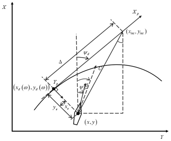
Figure 2.
Illustration of the LADLOS guidance law.
The use of the drift angle to pre-correct the desired heading angle is a common approach in the LOS guidance law. However, during the simulation of variable-speed trajectory tracking in this paper, it is observed that under low-speed and high-disturbance conditions, the vessel’s longitudinal speed and lateral speed are similar in magnitude. The drift angle can easily lead to differential peak phenomena with rapid changes, causing the drift angle to dominate the reference angle , resulting in system instability and making trajectory tracking difficult. The underlying issue lies in the fact that the drift angle is corrected based on speed rather than displacement. Since speed is the derivative of displacement, becomes highly sensitive to changes in the lateral speed at low speeds. To address this, a first-order inertia element is introduced to filter the drift angle , with the discrete first-order inertial filter given by Equation (9):
In this context, and denote the filtered drift angle at the previous time step and current time step, respectively. is the raw drift angle calculated at the current time. denotes the time constant of the first-order inertia element. denotes the sampling period of the discrete system. By applying the first-order inertial filter to smooth the drift angle, abrupt changes in the yaw angle are avoided, which prevents sharp variations in the rudder angle during heading control, thereby making the approach more consistent with engineering practice.
In the trajectory tracking of an underactuated vessel, as the desired point continuously advances, the moving speed depends on the rate of change of the parameters . The trajectory tracking controller controls the vessel to track the desired point with speed U and yaw angle . Once the vessel reaches the desired trajectory, it remains on the trajectory and moves forward at the desired speed. Therefore, the rate of change of the parameter not only determines the magnitude of the reference angle but also determines whether the vessel can track the desired trajectory at the desired speed.
Lemma 1.
For any smooth parameterized tracking trajectory , if the trajectory variation rate is chosen as , the vessel’s yaw angle will converge to the reference angle , and the vessel will converge to the desired trajectory at the desired speed. Here, , . and denote the first-order derivatives of the reference trajectory with respect to the parameter . denotes a positive constant, and denotes the longitudinal tracking error.
Proof of Lemma 1.
Let the desired position of the underactuated vessel be denoted as . The longitudinal tracking error and lateral tracking error for trajectory tracking in the body coordinate system {b} are given by Equation (10):
Here, and denote the longitudinal tracking error and the lateral tracking error in the {b} coordinate system. denotes the angle of the desire trajectory. Taking the derivatives of and , we obtain:
Here, , . The trajectory variation rate is defined as , with .
Select the Lyapunov function given by Equation (12):
Taking the derivative of Equation (12), we obtain
Define , where the purpose of the heading control is to converge the vessel’s yaw angle to the reference angle ; hence, . Combining with Equation (7), it can be derived that . Therefore,
Substituting Equation (14) into Equation (13), we obtain
Due to the properties of trigonometric functions, we obtain . Thus,
Moreover, since , we obtain
From the above, it can be concluded that , and , asymptotically converge to 0. □
In the heading control process, as the lateral tracking error decreases, the vessel’s yaw angle approaches the reference angle , ultimately aligning the vessel’s yaw angle with the angle of the desired trajectory , thus achieving heading control. In the speed control process, as the longitudinal tracking error decreases, the speed of the desired point on the desired trajectory aligns with the vessel’s motion speed, meaning that the desired point and the vessel move forward at the same speed.
In the speed control process, the selection of the desired speed profile is critical for control performance. In dynamic and complex scenarios, such as in the precise operations of a vessel in port, the flexible working requirements of the motors necessitate smooth speed variations, a fast dynamic response, and system stability. In this context, the seven-segment S-curve acceleration/deceleration process has become the ideal choice [32,33]. By introducing continuous changes in the acceleration and jerk, this method not only effectively avoids the vibration issues caused by abrupt changes in acceleration in traditional methods but also significantly improves the smoothness of trajectory tracking and the control accuracy. Furthermore, the S-curve design provides flexible parameter adjustment capabilities, allowing the system to find the optimal balance between response speed and comfort based on the actual task requirements. This smooth-speed planning approach ensures the system’s robustness against environmental disturbances and mitigates the adverse effects of nonlinear dynamics on control performance. Therefore, the seven-segment S-curve acceleration/deceleration process, with its high dynamic performance, excellent smoothness, and strong engineering feasibility, has become the ideal method for generating the desired velocity in control systems, providing a stable and efficient input foundation for subsequent controller design.
The seven stages of the S-curve acceleration/deceleration process are as follows: jerk acceleration phase (T1), uniform acceleration phase (T2), deceleration acceleration phase (T3), constant velocity phase (T4), acceleration–deceleration phase (T5), uniform deceleration phase (T6), and jerk deceleration phase (T7), as shown in Figure 3. In this paper, the variable is introduced to represent the rate of change of acceleration.
Based on the vessel’s propulsion characteristics, the maximum acceleration is denoted as , and a variable is introduced to represent the operating time in the current stage. The operating time for each stage, namely T1, T2, T3, T5, T6, and T7, is . The calculation formula for the S-curve acceleration process is given by Equation (19):
The calculation formula for the S-curve deceleration process is given by Equation (20):
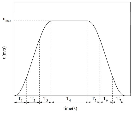
Figure 3.
S-curve acceleration and deceleration.
3. Adaptive Sliding Mode Controller
In Section 2, based on the underactuated vessel’s motion model, this paper employs the LADLOS method to compute the desired heading angle and designs a desired speed profile that follows the S-curve acceleration/deceleration process, laying the foundation for trajectory tracking control. However, in real maritime environments, vessel motion is inevitably affected by complex external disturbances, such as wind, waves, and currents, which exhibit uncertainty and dynamic characteristics. Therefore, in this section, the focus is on addressing the trajectory tracking control problem under the influence of unknown disturbances. To tackle these challenges, an ESO is first used to estimate unknown environmental disturbances. To ensure system stability during the progressive estimation process, even in the presence of observation errors, an adaptive control law is applied to estimate the upper bound of the unknown disturbances. Furthermore, the estimated disturbance results are used as feedforward compensation in the SMC, and an adaptive sliding mode control law based on the hyperbolic tangent function is designed to replace the traditional sign function. This approach smooths the control input and avoids high-frequency chattering. Finally, the TD3 algorithm is introduced for real-time tuning of the SMC parameters. This control strategy significantly enhances the system’s robustness and trajectory tracking performance.
3.1. Extended State Observer (ESO)
In the trajectory tracking of underactuated vessels, traditional control methods struggle to achieve sufficient accuracy in the state estimation and dynamic feedback due to external disturbances in the complex marine environment as well as the nonlinear characteristics and modeling uncertainties inherent in the vessel’s system. This results in degraded control performance. To address this issue, the ESO [34] is introduced as an effective auxiliary tool. The ESO is designed to estimate the system’s state variables and external disturbances in real time, thereby providing more precise feedback signals for the controller. The fundamental idea behind designing the ESO is to model the system’s dynamic characteristics and external disturbances as an “extended state”, which is then estimated by the observer. The uncertainties of the vessel and external environmental disturbances, such as wind and waves, are unified as unknown disturbance terms in the system. An ESO is used to observe the vessel’s states and unknown disturbances. Let , , , , and . Considering the underactuated vessel model, the design of the ESO is given by Equation (21):
Here, , and . denotes the observed value of speed, and denotes the observed value of . is the design positive constant, and it denotes the gain of the ESO. Typically, . denotes the bandwidth, which is determined by the frequency of the disturbance signal to be observed.
Define the observation error as , where , and . Combining Equations (1), (2) and (21), the state equation for the observation error is given by Equation (22):
Clearly, by solving the differential equation in Equation (22), we obtain
From Assumption 2, it follows that , where is a positive design constant. For the matrix , there exists a Vandermonde matrix that satisfies the following relationship: . Therefore,
From , it is known that as , . According to Equation (24), the convergence of is related to the bandwidth value . The larger the bandwidth, the faster the convergence, and it will ultimately converge to the boundary value . Therefore, the observation error of the disturbance estimated by the ESO is convergent and will eventually converge to the boundary value.
3.2. Heading and Speed Sliding Mode Control
The core idea of SMC is to design a sliding surface such that the system’s state converges to this surface and remains on it, thereby achieving the desired trajectory tracking. In this paper, the states of the underactuated vessel are defined as the speed error and heading error, with the calculation formulas given by Equation (25):
Design the sliding surfaces given by Equation (26) and Equation (27), respectively.
Considering the underactuated vessel model and taking the time derivative of Equations (26) and (27), the results are given by Equations (28) and (29).
Based on the SMC concept, the control laws are given by Equations (30) and (31).
Here, , , , and are positive constants. In the equation, the is used to replace the in the traditional SMC.
Theorem 1.
For the underactuated vessel motion model given by Equations (1) and (2), under the conditions specified in Assumptions 1 and 2, and given the desired trajectory and the desired speed profile, the SMC laws for thrust (Equation (30)) and steering torque (Equation (31)) are designed, and the boundary values of external environmental disturbances are estimated. By appropriately selecting the parameters , , , , , and , it can be guaranteed that the underactuated vessel will track the desired trajectory with the desired speed, and that all states of the trajectory tracking system are ultimately uniformly bounded.
Proof of Theorem 1.
Construct the Lyapunov function given by Equation (32).
Here, and denote the estimated values of and , respectively. and denote the observation errors of the disturbance bounds of the vessel’s external disturbances. Taking the derivative of the Lyapunov function yields
Substituting Equations (28) and (29), we obtain
Here, , and . The adaptive laws for designing and are formulated as follows [35]:
In Equation (35), , , , and are positive design constants, while and are small. , . is a positive design constant. and denote the prior estimates of and , respectively. Substituting Equation (35) into Equation (34), we obtain
Moreover, due to the properties of , it can be concluded that
For any positive constants , , we obtain [36]
Taking into account the inequality given by Equation (39),
Substituting Equation (39) into Equation (37), we obtain
Here,
From the above equation, it can be concluded that when . Thus, the system achieves stability. Therefore, the signals , , , and in the closed-loop system are uniformly ultimately bounded. It can also be concluded that and are bounded. By combining Equation (17), it can be ensured that the vessel’s trajectory tracking error is uniformly ultimately bounded. □
3.3. TD3 Algorithm Parameter Optimization
TD3 is an efficient, policy-gradient-based algorithm in the field of deep reinforcement learning, specifically designed for continuous action space problems. The core of TD3 lies in the use of a deterministic policy and an actor–critic architecture to approximate the optimal policy. The primary objective is to learn the optimal policy through interactions with the environment, thereby maximizing the cumulative reward. The TD3 algorithm is an optimized version of the Deep Deterministic Policy Gradient (DDPG) algorithm. It utilizes two separate critic networks, and when computing the target value, the smaller of the two is chosen, effectively mitigating the overestimation issue found in the DDPG. Additionally, random noise is introduced into the action of the next state during target value computation, enhancing the accuracy of value estimation. Finally, the actor network is updated only after multiple updates to the critic network, ensuring stability in actor network training. The parameter optimization structure based on TD3 is shown in Figure 4.
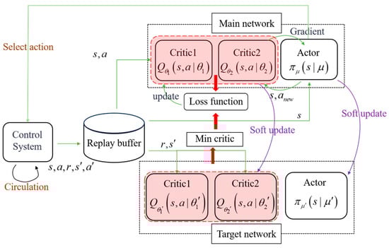
Figure 4.
TD3 parameter optimization structure.
The TD3 environment constructed in this paper consists of an underactuated vessel model and a sliding mode controller. The state space and action space are defined as follows: and . The state variables reflect the longitudinal tracking error, lateral tracking error, yaw tracking error, and speed tracking error. The action space denotes the parameters of the sliding mode controller that need to be optimized. The objective of trajectory tracking for the underactuated vessel is to minimize the error between the vessel’s state and the desired state. As the trajectory moves toward the target trajectory, the longitudinal tracking error, lateral tracking error, yaw tracking error, and speed tracking error should gradually approach zero. Therefore, the reward function is designed as follows:
denotes a small positive constant, which is used to prevent the issue of infinite rewards when the state variables are all zero. The TD3 algorithm includes six neural networks, and the parameters of the neural networks are set as shown in Table 1.

Table 1.
Network structure.
4. System Control Structure
To address the trajectory tracking problem of underactuated vessels, this paper proposes a sliding mode controller optimized by the TD3 algorithm. The overall control structure is shown in Figure 5. The system input is the desired trajectory and speed , while the outputs are the vessel’s actual state. The method involves constructing two control subsystems to achieve precise control of the speed and the yaw angle, thereby fulfilling the trajectory tracking control objective. The control system takes the speed tracking error and yaw tracking error as control state inputs and designs an integral sliding mode surface for speed control and a differential sliding mode surface for heading control. Based on the sliding mode surface feedback control strategy, the system outputs the longitudinal thrust and steering torque, ensuring that the longitudinal tracking error and the lateral tracking error gradually converge to achieve accurate tracking of the desired trajectory. To handle external and model uncertainties, an ESO is introduced to observe and compensate for the compound disturbances in real time, and an adaptive law is designed to estimate the upper bound of the unknown disturbances, ensuring system stability even in the presence of gradual observation errors. To further optimize the performance of the sliding mode controller, the TD3 algorithm is utilized to optimize the control parameters. The TD3 algorithm is an enhanced version of the DDPG algorithm, mitigating the value overestimation issue present in the DDPG, and employing a delayed update strategy to ensure smoothness of the control parameter outputs and the stability of system dynamic responses.
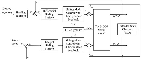
Figure 5.
Control system structure.
5. Simulation Results
To verify the effectiveness of the proposed method, a simulation is conducted on a recreational boat from Ningbo FlyShark Power Technology Co., Ltd, located in Ningbo, China. Considering the influence of hydrodynamic factors, the Inoue model [37] is introduced to calculate the viscous forces generated by the system, as shown in Equation (43). , , , , , , , , , , , , , and denote hydrodynamic coefficients, and in practical applications, their dimensionless forms are often calculated using empirical formulas. The Zhou Zhaoming formula [38] is used to calculate the additional inertial forces generated by the system, with the corresponding formula provided in Equation (44). , , and denote the additional mass in the X and Y directions and additional moment of inertia in the Z direction, respectively. denotes the moment of inertia about the Z-axis. The dimensionless parameters of the model and the hydrodynamic parameters obtained from the calculations are listed in Table 2, where the “dash” data represents the dimensionless data. The parameters for the TD3 algorithm are set as follows: , , , , .
Table 2.
Main data of the ship model.
5.1. Maneuverability Analysis
Simulation tests are conducted to evaluate the operability of the constructed model. The impacts of thrust and torque on the vessel’s motion state are tested, as these are key factors for achieving trajectory tracking control of an underactuated vessel.
Under the condition that both the initial velocity and torque are 0, the thrust is input as follows: 10 N, 50 N, 100 N, 200 N, 500 N, 1000 N. The simulation results show that as the thrust increases, the vessel’s forward speed also increases accordingly, as shown in Figure 6a. As the thrust increases, the forward speed of the vessel gradually approaches a stable value. Specifically, with thrust inputs of 10 N, 50 N, 100 N, 200 N, 500 N, and 1000 N, the vessel’s final forward velocities stabilize at 0.15 m/s, 0.25 m/s, 0.5 m/s, 1.1 m/s, and 1.55 m/s, respectively. Under the condition of an initial velocity of 0 and a thrust of 100 N, the thrust inputs are as follows: −100 N, −50 N, 50 N, and 100 N, with the simulation results shown in Figure 6b. Specifically, when the torque is ±50 N, the vessel’s turning radius is approximately 5 m, and when the torque is ±100 N, the turning radius is approximately 14 m. Moreover, the vessel’s rotation direction is opposite to the sign of the applied torque. When the torque is positive, the vessel rotates counterclockwise. When the torque is negative, the vessel rotates clockwise. The simulation results lead to the conclusion that the vessel’s motion control can be achieved by adjusting the magnitude of the thrust and torque. The established vessel model is consistent with the actual operational behavior of vessels, effectively simulating the vessel’s motion state under different control inputs and providing a reliable basis for trajectory tracking control simulations.
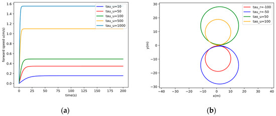
Figure 6.
Maneuverability validation. (a) Forward speed under different thrusts. (b) Trajectory under different torques.
5.2. Sine Wave Trajectory Tracking Simulation
This section presents the trajectory tracking control simulations for a sine trajectory. The equation of the sine trajectory to be tracked is . Based on Assumption 2, the disturbance is set as shown in Equation (45):
Let the initial position of the vessel be , and the initial velocity of the vessel be . The action space range is set to and , with the other parameters set to . To verify the impact of the drift angle on the vessel’s heading control, a series of simulation experiments are conducted, and the results are shown in Figure 7. In the early stages of the vessel’s operation, the influence of the drift angle on the reference angle is significant. The maximum error between the reference angle calculated through drift angle filtering and the reference angle obtained by removing the drift angle can reach 0.4 rad. Furthermore, it can also be observed that when the trajectory curvature is large, the method of calculating the reference angle by removing the drift angle introduces errors compared with the method that calculates the reference angle through drift angle filtering. Therefore, it is particularly important to use filtering techniques to smooth the drift angle. A low-pass filter is used to smooth the drift angle, and the desired heading angle of the vessel varies smoothly. With the presence of the drift angle, higher control accuracy is achieved. In summary, the drift angle has a significant impact on the trajectory tracking performance of underactuated vessels, especially in the initial heading control phase. Therefore, it is necessary to use appropriate filtering techniques to process the drift angle, improving the vessel’s heading accuracy and trajectory tracking stability. Considering the drift angle filtering, the vessel’s trajectory tracking simulation results are shown in Figure 8, Figure 9, Figure 10, Figure 11 and Figure 12. Figure 8a shows the sliding mode controller parameters obtained through the TD3 algorithm.
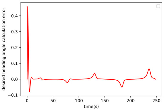
Figure 7.
Effect of the drift angle on the reference angle.
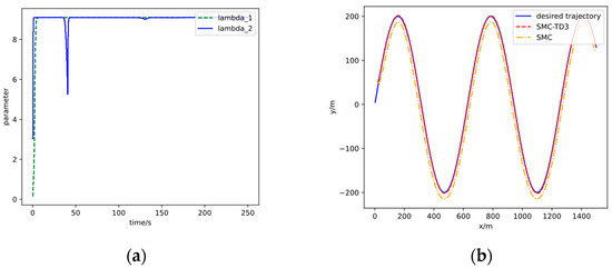
Figure 8.
Control parameters and trajectory comparison of the sine trajectory. (a) Control parameters. (b) Trajectory comparison.
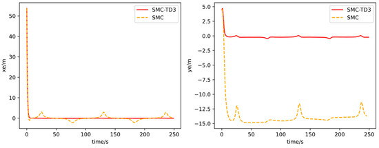
Figure 9.
Longitudinal tracking error and lateral tracking error of the sine trajectory.
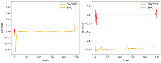
Figure 10.
Speed tracking error and yaw tracking error of the sine trajectory.
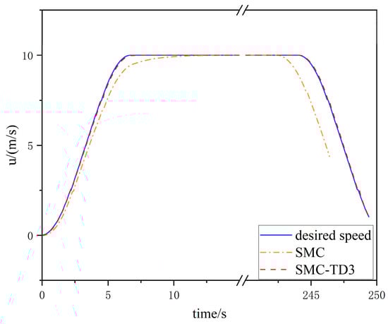
Figure 11.
Variable speed tracking of the sine trajectory.
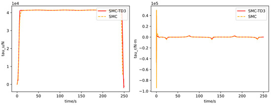
Figure 12.
Control force of the sine trajectory.
When the SMC parameters are set to and , the actual operating trajectory of the SMC is shown by the orange curve in Figure 8b. The actual operating trajectory of the sliding mode controller optimized by the TD3 algorithm (SMC-TD3) in real time is shown by the red curve in Figure 8b. Comparing both trajectories with the desired trajectory, the results indicate that the SMC-TD3 performs better in tracking the desired trajectory. It is able to track the desired path more quickly and with smaller tracking errors. Figure 9 presents a comparison of the longitudinal tracking error and the lateral tracking error in the SMC and the SMC-TD3. It can be observed that the longitudinal tracking error of the SMC stabilizes within the range of [−3, 3], while the longitudinal tracking error of the SMC-TD3 converges to 0. This indicates that the SMC-TD3 achieves smaller longitudinal tracking errors. Both methods exhibit bounded lateral tracking errors. The lateral tracking error of the SMC stabilizes within the range of [−15, −12.5], whereas the lateral tracking error of the SMC-TD3 stabilizes within the range of [−1, 1], showing that the SMC-TD3 achieves smaller lateral tracking errors. Figure 10 shows a comparison of the speed tracking error and the yaw tracking error in the SMC and the SMC-TD3. The speed tracking errors of both methods converge to 0. Both methods also exhibit convergence of the yaw tracking error. The SMC’s yaw tracking error converges to −0.8, while the SMC-TD3’s yaw tracking error converges to 0. Comparing the two methods, the SMC-TD3 demonstrates superior overall control performance. Figure 11 illustrates the speed control performance of both the SMC and the SMC-TD3. Both methods are capable of achieving variable-speed tracking control for the underactuated vessel. Figure 12 displays the control force variations for both controllers. While both methods ensure smooth control of the underactuated vessel, the SMC-TD3 exhibits smoother control. Therefore, the SMC-TD3 is better suited to meet the practical engineering control requirements.
5.3. Circular Trajectory Tracking Simulation
This section describes the trajectory tracking control simulation performed for a circular trajectory. The equation of the circular trajectory to be tracked is given by Equation (46), and the external disturbance is set as shown in Equation (45):
Let the initial position of the vessel be , and the initial vessel speed be m/s. Set the action space as and, , with the other parameters as . The vessel’s trajectory tracking results are shown in Figure 13, Figure 14, Figure 15, Figure 16 and Figure 17. The SMC parameters obtained through the TD3 algorithm are shown in Figure 13a.
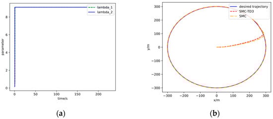
Figure 13.
Control parameters and trajectory comparison of the circular trajectory. (a) Control parameters. (b) Trajectory comparison.
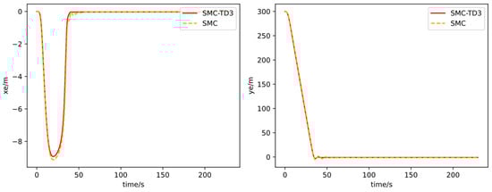
Figure 14.
Longitudinal tracking error and lateral tracking error of the circular trajectory.
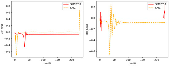
Figure 15.
Speed tracking error and yaw tracking error of the circular trajectory.
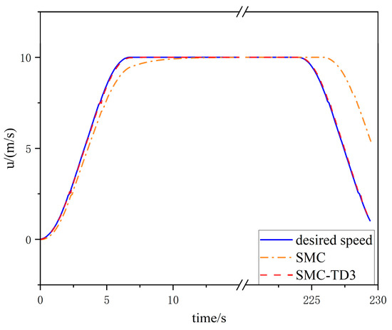
Figure 16.
Variable speed tracking of the circular trajectory.
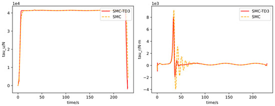
Figure 17.
Control force of the circular trajectory.
When the sliding mode control parameters are set to and , the actual operating trajectory of the SMC is shown by the orange line in Figure 13b. The actual operating trajectory of the SMC-TD3 is shown by the red line in Figure 13b. A comparison of the two trajectories with the desired trajectory shows that SMC-TD3 performs better in trajectory tracking, enabling faster convergence to the desired path. Figure 14 presents the comparison of the longitudinal tracking error and lateral tracking error in the SMC and the SMC-TD3. It can be observed that both methods lead to the longitudinal tracking error and lateral tracking error approaching zero. However, the SMC-TD3 exhibits a smoother tracking performance. Figure 15 shows a comparison of the speed tracking error and yaw tracking error in the SMC and the SMC-TD3. Both methods exhibit bounded speed tracking errors. The SMC’s speed tracking error converges to −0.1, while the SMC-TD3’s speed tracking error converges to 0. Both methods show bounded yaw tracking errors. The SMC’s yaw tracking error converges to 0, while the SMC-TD3’s yaw tracking error converges to −0.1. However, the SMC-TD3 demonstrates a faster dynamic response. Figure 16 illustrates the speed control performance of both the SMC and the SMC-TD3. Both methods are capable of achieving variable-speed tracking control for the underactuated vessel. Figure 17 presents the control force variations for the SMC and the SMC-TD3. It can be observed that the SMC-TD3 exhibits smoother control compared with the SMC method. Furthermore, the control force of the SMC-TD3 is smoother, better meeting the practical engineering control requirements.
6. Conclusions
This paper investigates the problem of variable-speed trajectory tracking control for underactuated vessels. First, considering the hydrodynamic effects on the underactuated ship, a 3-DOF motion model of the underactuated vessel is established. Next, based on the motion model, two sliding mode controllers are designed: a speed sliding mode controller and a heading sliding mode controller. For speed control, the desired speed is designed to follow an S-curve acceleration/deceleration process in accordance with the variable-speed tracking control requirements of the underactuated vessel. For heading control, the LADLOS method is used to dynamically calculate the desired heading angle of the underactuated vessel. To address external composite disturbances, an ESO is designed to observe and compensate for the disturbances in real-time. An adaptive law is also designed to estimate the error bounds, and the global stability of the system is proven using the Lyapunov method. Third, to further optimize the performance of the sliding mode controller, the TD3 algorithm is introduced for parameter tuning. Additionally, due to the dynamic characteristics of the underactuated vessel’s propulsion system, the phenomenon of sudden changes in the drift angle often occurs when the vessel starts, and this drift angle can affect the heading control. To address the drift angle issue, a first-order inertial element filter is introduced to smooth the drift angle data. Numerical simulation results demonstrate that the proposed method significantly improves the trajectory tracking accuracy and dynamic response speed of the underactuated vessel. Specifically, for the sinusoidal trajectory with an amplitude of 200 m and a frequency of 0.01, numerical results show that the proposed method achieves convergence of the longitudinal tracking error to zero, while the lateral tracking error remains stable within 1 m. For the circular trajectory with a radius of 300 m, the numerical results indicate that both the longitudinal and lateral tracking errors are stabilized within 1 m. Compared with the fixed-value sliding mode controller, the proposed method demonstrates superior trajectory tracking accuracy and smoother control performance.
Author Contributions
Conceptualization, S.Z.; Methodology, S.Z.; Software, Z.L.; Resources, Q.W.; Data curation, Q.W.; Writing—original draft, S.Z.; Writing—review & editing, G.Z.; Visualization, Z.L.; Supervision, G.Z. All authors have read and agreed to the published version of the manuscript.
Funding
This research was supported by the Nature Science Fund Project of Zhejiang Province. The funding number is LGN21C190007. This research was supported by the Nature Science Fund Project of Ningbo. The funding number is 202003N4074.
Institutional Review Board Statement
Not applicable.
Informed Consent Statement
Not applicable.
Data Availability Statement
Data are contained within the article.
Acknowledgments
The authors would like to thank the funder for supporting them and the editor and reviewers for their constructive comments.
Conflicts of Interest
The authors declare no conflicts of interest.
References
- Zhang, W.; Liao, Y.L.; Jiang, F.; Zhao, T.J. Development Review and Trend Analysis of Unmanned Surface Vehicles Technology. Unmanned Syst. Technol. 2019, 2, 1–9. [Google Scholar]
- Cong, X.; Zhao, C. PID control of uncertain nonlinear stochastic systems with state observer. Sci. China Inf. Sci. 2021, 64, 192201. [Google Scholar] [CrossRef]
- Liu, Z.Q.; Chi, R.H.; Huang, B.; Hou, Z.S. Finite-time PID control for nonlinear nonaffine systems. Sci. China Inf. Sci. 2024, 67, 212206. [Google Scholar] [CrossRef]
- Lyu, X.J.; Lin, Z.L. PID Control of Planar Nonlinear Uncertain Systems in the Presence of Actuator Saturation. IEEE/CAA J. Autom. Sin. 2022, 9, 90–98. [Google Scholar] [CrossRef]
- Liu, S.W.; Zuo, Y.; Li, T.S.; Wang, H.Q.; Gao, X.Y.; Xiao, Y. Adaptive fixed-time PID-based control of uncertain nonlinear systems and its application to unmanned surface vehicles. Int. J. Syst. Sci. 2024, 55, 2815–2824. [Google Scholar] [CrossRef]
- Zhao, C. Semiglobal stability of PID for uncertain nonaffine systems. Automatica 2024, 160, 111429. [Google Scholar] [CrossRef]
- Saleem, O.; Iqbal, J. Fuzzy-Immune-Regulated Adaptive Degree-of-Stability LQR for a Self-Balancing Robotic Mechanism: Design and HIL Realization. IEEE Robot. Autom. Lett. 2023, 8, 4577–4584. [Google Scholar] [CrossRef]
- Xin, G.Y.; Xin, S.T.; Cebe, O.; Pollayil, M.J.; Angelini, F.; Garabini, M.; Vijayakumar, S.; Mistry, M. Robust Footstep Planning and LQR Control for Dynamic Quadrupedal Locomotion. IEEE Robot. Autom. Lett. 2021, 6, 4488–4495. [Google Scholar] [CrossRef]
- Ali, N.; Ayaz, Y.; Iqbal, J. Collaborative Position Control of Pantograph Robot Using Particle Swarm Optimization. Int. J. Control Autom. Syst. 2022, 20, 198–207. [Google Scholar] [CrossRef]
- Choubey, C.; Ohri, J. Tuning of LQR-PID controller to control parallel manipulator. Neural Comput. Appl. 2022, 34, 3283–3297. [Google Scholar] [CrossRef]
- Yuan, Y.; Wang, Y.J.; Guo, L. Sliding-Mode-Observer-Based Time-Varying Formation Tracking for Multispacecrafts Subjected to Switching Topologies and Time-Delays. IEEE Trans. Automat. Control 2021, 66, 3848–3855. [Google Scholar] [CrossRef]
- Um, Y.-C.; Choi, H.-L. Integral γ-Sliding Mode Control for a Quadrotor with Uncertain Time-Varying Mass and External Disturbance. J. Electr. Eng. Technol. 2022, 17, 707–716. [Google Scholar] [CrossRef]
- Hou, H.Z.; Yu, X.H.; Fu, Z. Sliding-Mode Control of Uncertain Time-Varying Systems With State Delays: A Non-Negative Constraints Approach. IEEE Trans. Syst. Man Cybern Syst. 2022, 52, 1516–1524. [Google Scholar] [CrossRef]
- Weng, Y.P.; Wang, N. Finite-time observer-based model-free time-varying sliding-mode control of disturbed surface vessels. Ocean Eng. 2022, 251, 110866. [Google Scholar] [CrossRef]
- Davila, J.; Tranninger, M.; Fridman, L. Finite-Time State Observer for a Class of Linear Time-Varying Systems With Unknown Inputs. IEEE Trans. Autom. Control 2022, 67, 3149–3156. [Google Scholar] [CrossRef]
- Mao, Z.H.; Yan, X.-G.; Jiang, B.; Spurgeon, S.K. Sliding Mode Control of Nonlinear Systems With Input Distribution Uncertainties. IEEE Trans. Autom. Control 2023, 68, 6208–6215. [Google Scholar] [CrossRef]
- Zhou, B.; Ding, Y.; Zhang, K.-K.; Duan, G.-R. Prescribed time control based on the periodic delayed sliding mode surface without singularities. Sci. China Inf. Sci. 2024, 67, 172204. [Google Scholar] [CrossRef]
- Wang, J.; Wang, H.T.; Yan, H.C.; Wang, Y.Y.; Shen, H. Fuzzy H∞ Sliding Mode Control of Persistent Dwell-Time Switched Nonlinear Systems. IEEE Trans. Fuzzy Syst. 2022, 30, 5143–5151. [Google Scholar] [CrossRef]
- Gurumurthy, G.; Das, D.K. Terminal sliding mode disturbance observer based adaptive super twisting sliding mode controller design for a class of nonlinear systems. Eur. J. Control 2021, 57, 232–241. [Google Scholar] [CrossRef]
- Zhao, L.; Li, Z.J.; Li, H.B.; Liu, B. Backstepping integral sliding mode control for pneumatic manipulators via adaptive extended state observers. ISA Trans. 2024, 144, 374–384. [Google Scholar] [CrossRef] [PubMed]
- Ahmadi, K.; Asadi, D.; Merheb, A.; Nabavi-Chashmi, S.-Y.; Tutsoy, O. Active fault-tolerant control of quadrotor UAVs with nonlinear observer-based sliding mode control validated through hardware in the loop experiments. Control Eng. Pract. 2023, 137, 105557. [Google Scholar] [CrossRef]
- Herman, P. A Quasi-Velocity-Based Tracking Controller for a Class of Underactuated Marine Vehicles. Appl. Sci. 2022, 12, 8903. [Google Scholar] [CrossRef]
- Zhu, T.B.; Xiao, Y.J.; Zhang, H.; Pan, Y.F. Trajectory Tracking Control of USV Based on Exponential Global Fast Terminal Sliding Mode Control. Proc. Inst. Mech. Eng. Part I J. Syst. Control Eng. 2024, 238, 47–58. [Google Scholar] [CrossRef]
- Wang, Y.; Du, Z.B. Trajectory Tracking Control for an Underactuated AUV via Nonsingular Fast Terminal Sliding Mode Approach. J. Mar. Sci. Eng. 2024, 12, 1442. [Google Scholar] [CrossRef]
- Xu, D.H.; Li, Z.L.; Xin, P.; Zhou, X.Q. The Non-Singular Terminal Sliding Mode Control of Underactuated Unmanned Surface Vessels Using Biologically Inspired Neural Network. J. Mar. Sci. Eng. 2024, 12, 112. [Google Scholar] [CrossRef]
- Wu, Z.W.; Peng, H.S.; Hu, B.; Feng, X.D. Trajectory Tracking of a Novel Underactuated AUV via Nonsingular Integral Terminal Sliding Mode Control. IEEE Access 2021, 9, 103407–103418. [Google Scholar] [CrossRef]
- Lei, Y.S.; Zhang, X.K. Ship trajectory tracking control based on adaptive fast non-singular integral terminal sliding mode. Ocean Eng. 2024, 311, 118975. [Google Scholar] [CrossRef]
- Sun, X.J.; Wang, G.F.; Fan, Y.S. Model Identification and Trajectory Tracking Control for Vector Propulsion Unmanned Surface Vehicles. Electronics 2019, 9, 22. [Google Scholar] [CrossRef]
- Zhang, Q.; Zhang, M.J.; Yang, R.M.; Im, N. Adaptive Neural Finite-time Trajectory Tracking Control of MSVs Subject to Uncertainties. Int. J. Control Autom. Syst. 2021, 19, 2238–2250. [Google Scholar] [CrossRef]
- Zhang, C.J.; Wang, C.; Wei, Y.J.; Wang, J.Q. Neural-Based Command Filtered Backstepping Control for Trajectory Tracking of Underactuated Autonomous Surface Vehicles. IEEE Access 2020, 8, 42481–42490. [Google Scholar] [CrossRef]
- Endo, M.; Hsegawa, K. Passage planning system for small inland vessels based on standard paradigms and maneuvers of experts. In Proceedings of the International Conference on Marien Simulation and Ship Manoeuvrability, Kanazawa, Japan, 25–28 August 2003. [Google Scholar]
- Cai, Z.F. A Fast Realization Method of S-shaped Acceleration and Deceleration Control Curve for Stepper Motor Based on STM32. Inf. Technol. Informatiz. 2014, 27–29+33. [Google Scholar]
- Baraldo, S.; Valente, A. Smooth joint motion planning for high precision reconfigurable robot manipulators. In Proceeding of the 2017 IEEE International Conference on Robotics and Automation (ICRA), Singapore, 29 May–3 June 2017. [Google Scholar] [CrossRef]
- Gao, Q.H.; Dong, J.C. Feedforward compensation design for observation error of extended state observer. J. Natl. Univ. Def. Technol. 2019, 41, 93–102. [Google Scholar]
- Sheng, Z.P. Adaptive Sliding Mode Control for Ship Motion; China Science Publishing & Media Ltd.: Beijing, China, 2019. [Google Scholar]
- Do, K.D.; Jiang, Z.J.; Pan, J. Robust adaptive path following of underactuated ships. Automatica 2004, 40, 929–944. [Google Scholar] [CrossRef]
- Jia, X.L.; Yang, T.S. Mathematical Models of Ship Motion: Mechanistic Modeling and Identification Modeling; Dalian Maritime University Press: Dalian, China, 1997. [Google Scholar]
- Zhou, Z.M.; Sheng, Z.Y.; Feng, W.S. Forecasting the Maneuverability of Multi-Purpose Cargo Ships. Ship Eng. 1983, 6, 21–29+36+4. [Google Scholar]
Disclaimer/Publisher’s Note: The statements, opinions and data contained in all publications are solely those of the individual author(s) and contributor(s) and not of MDPI and/or the editor(s). MDPI and/or the editor(s) disclaim responsibility for any injury to people or property resulting from any ideas, methods, instructions or products referred to in the content. |
© 2025 by the authors. Licensee MDPI, Basel, Switzerland. This article is an open access article distributed under the terms and conditions of the Creative Commons Attribution (CC BY) license (https://creativecommons.org/licenses/by/4.0/).