
Collaborative Transport Strategy for Dual AGVs in Smart Ports: Enhancing Docking Accuracy in No-Load Formations


Abstract
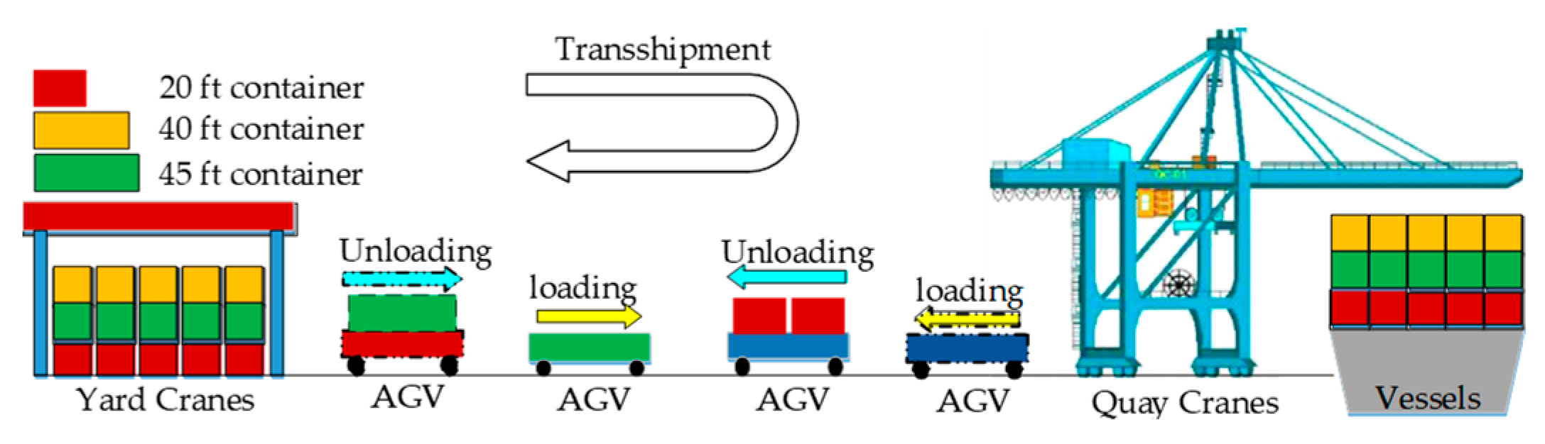
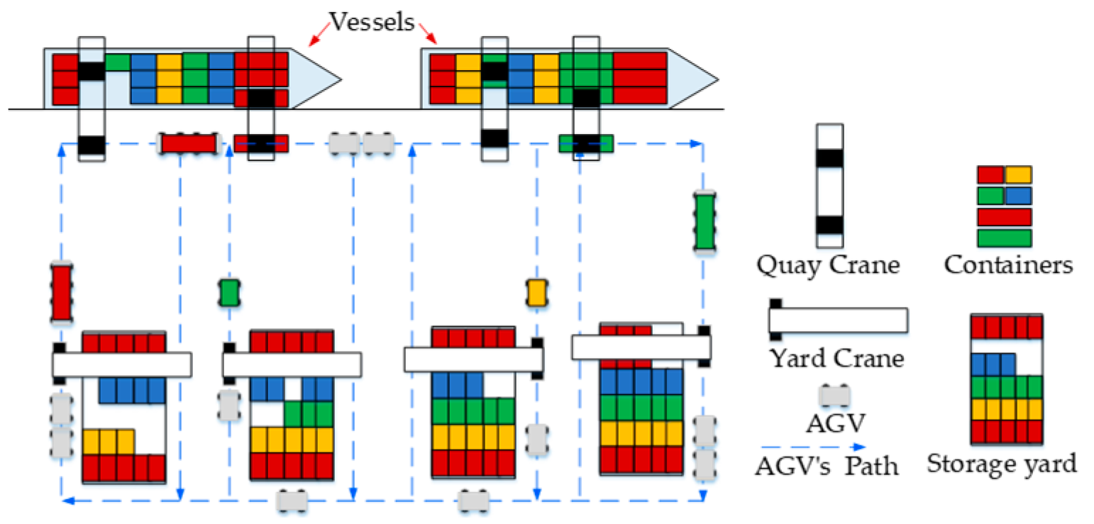
1. Introduction
2. Preliminary Knowledge
3. System Modeling
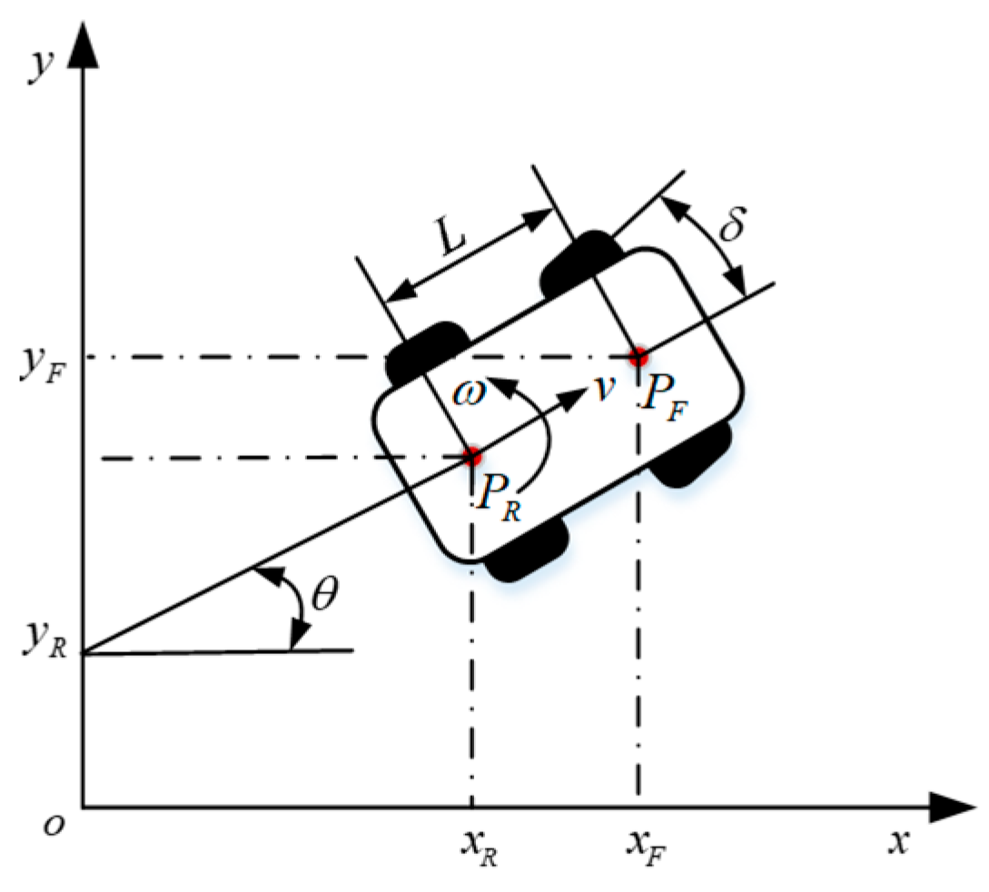
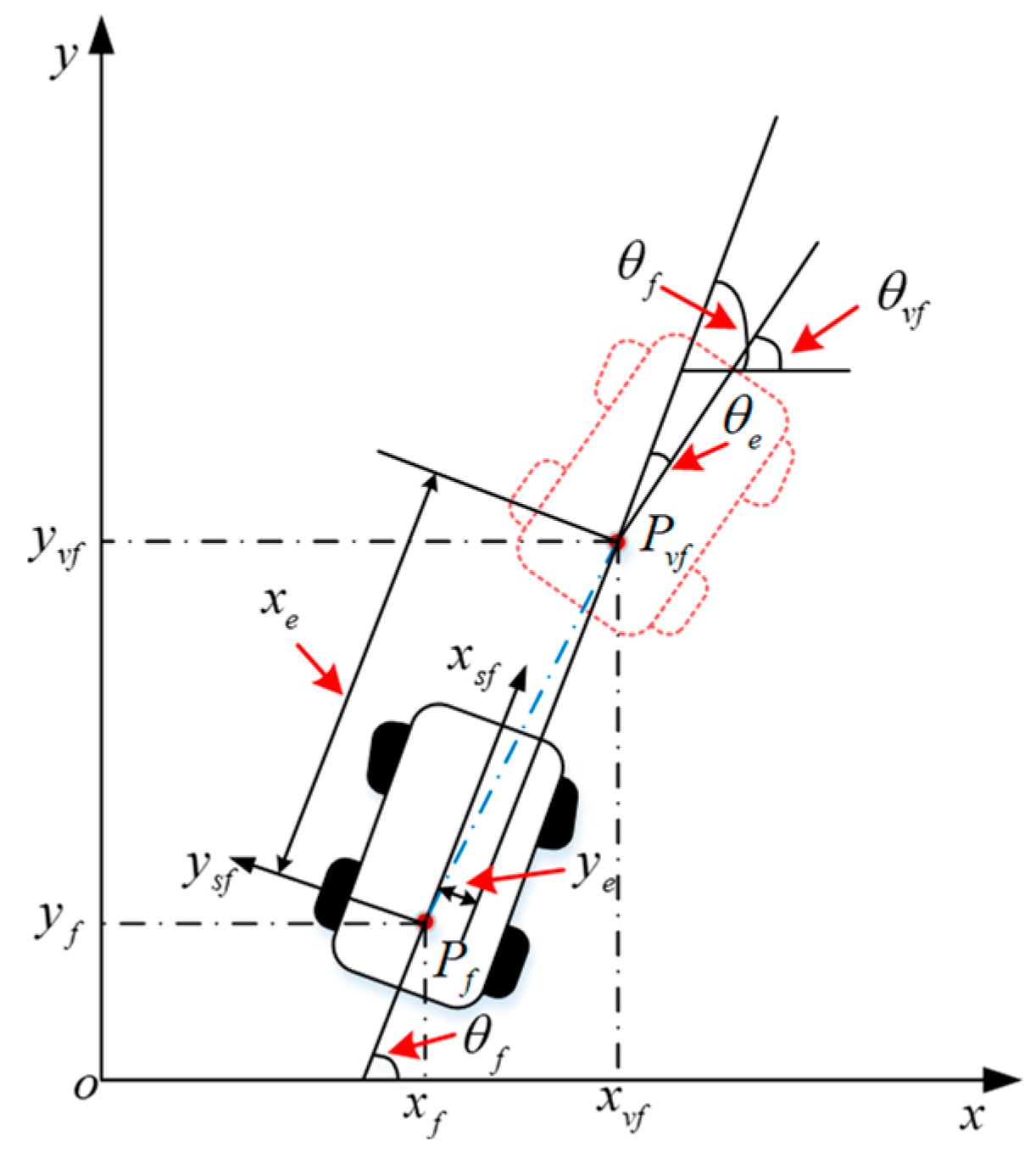
3.1. The Kinematic Model of a Single AGV
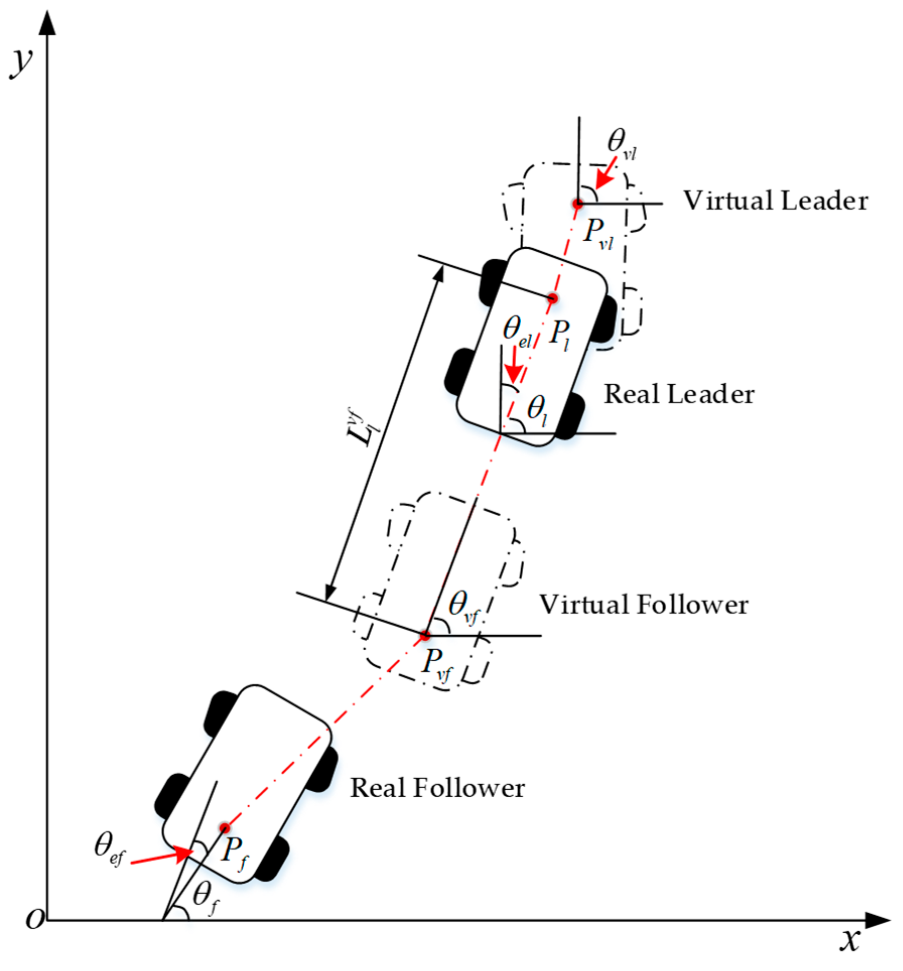
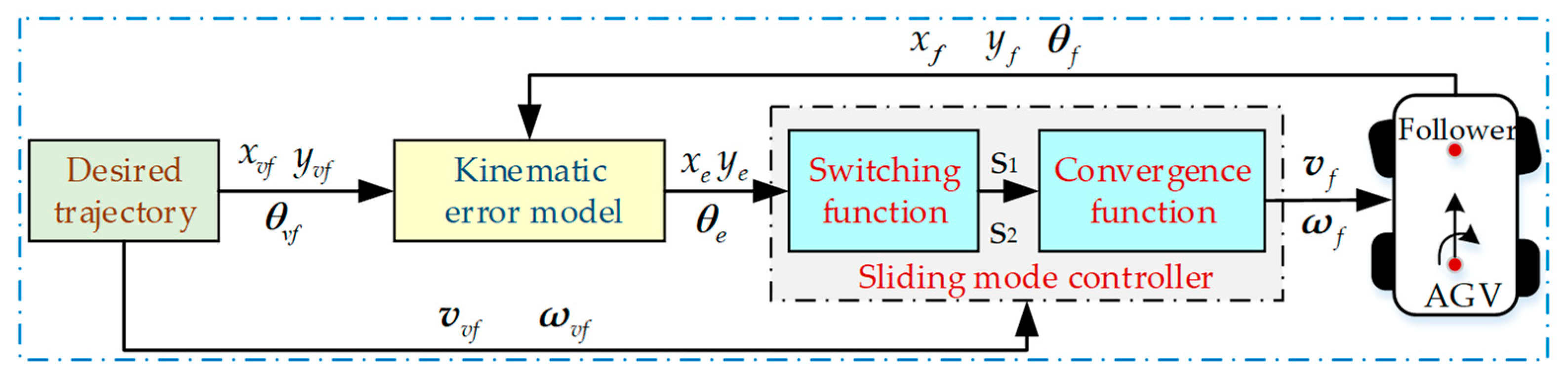
3.2. Feedback Mechanism of the Formation
4. Innovative Controller Design
5. Simulations and Analysis
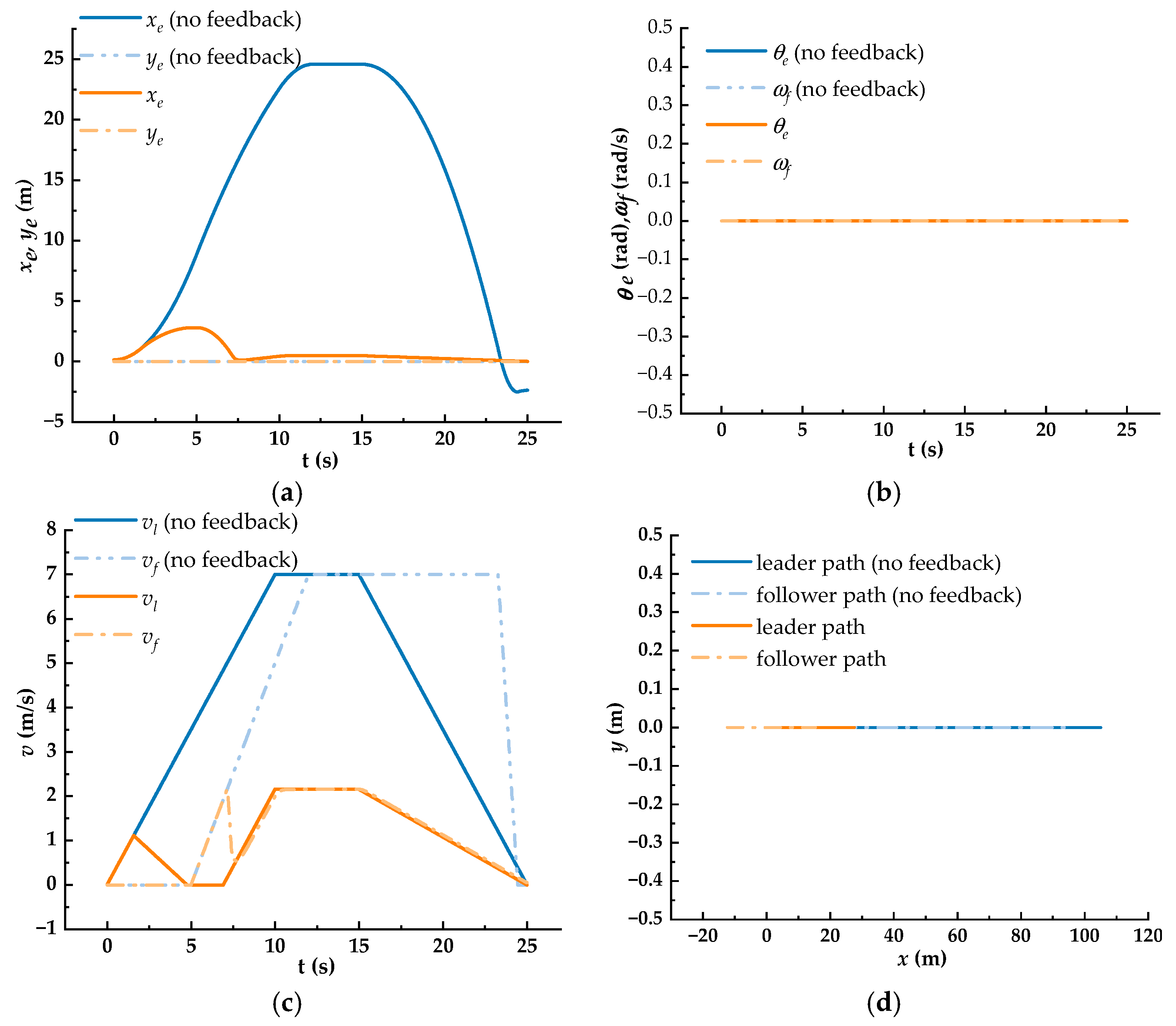
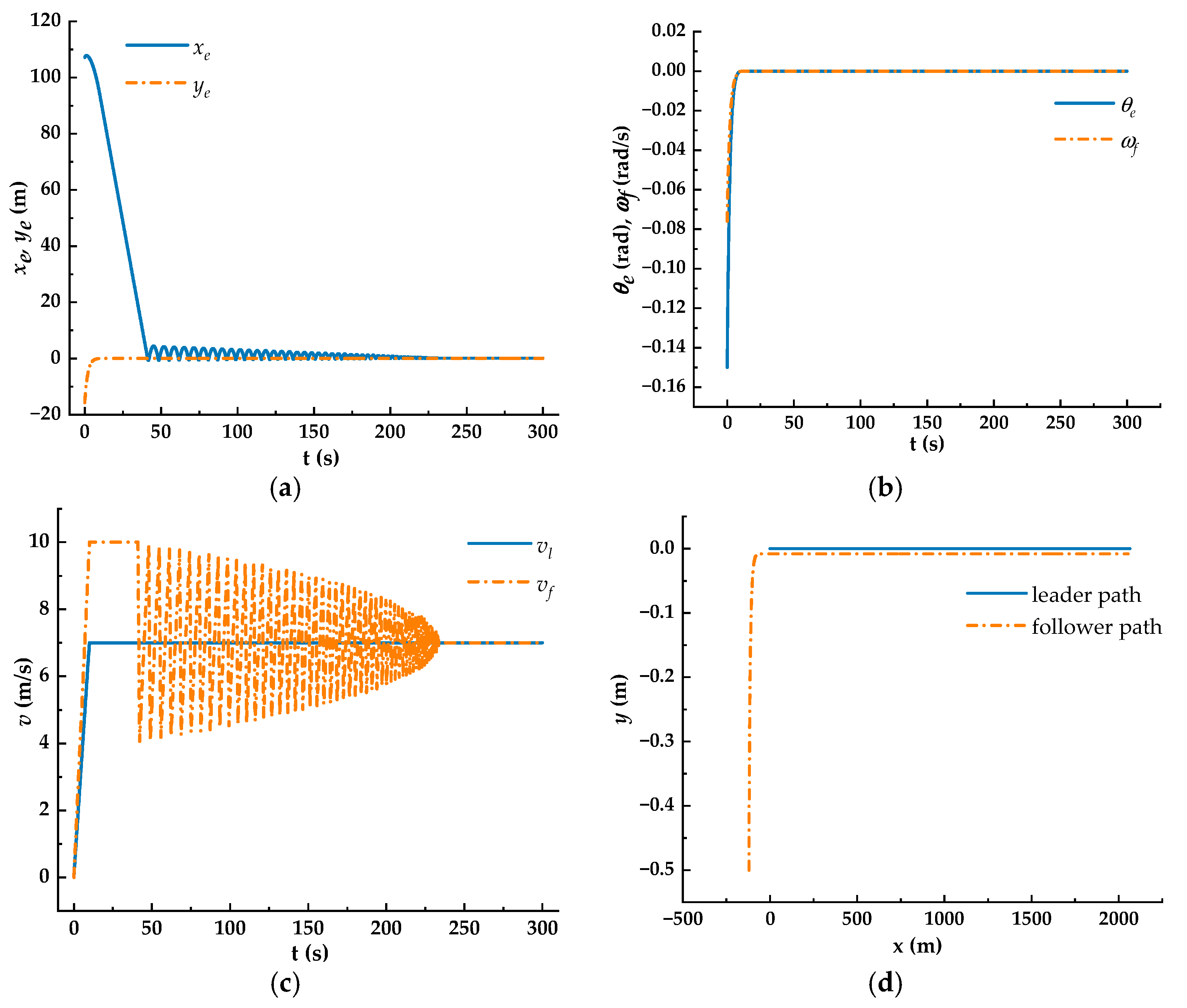
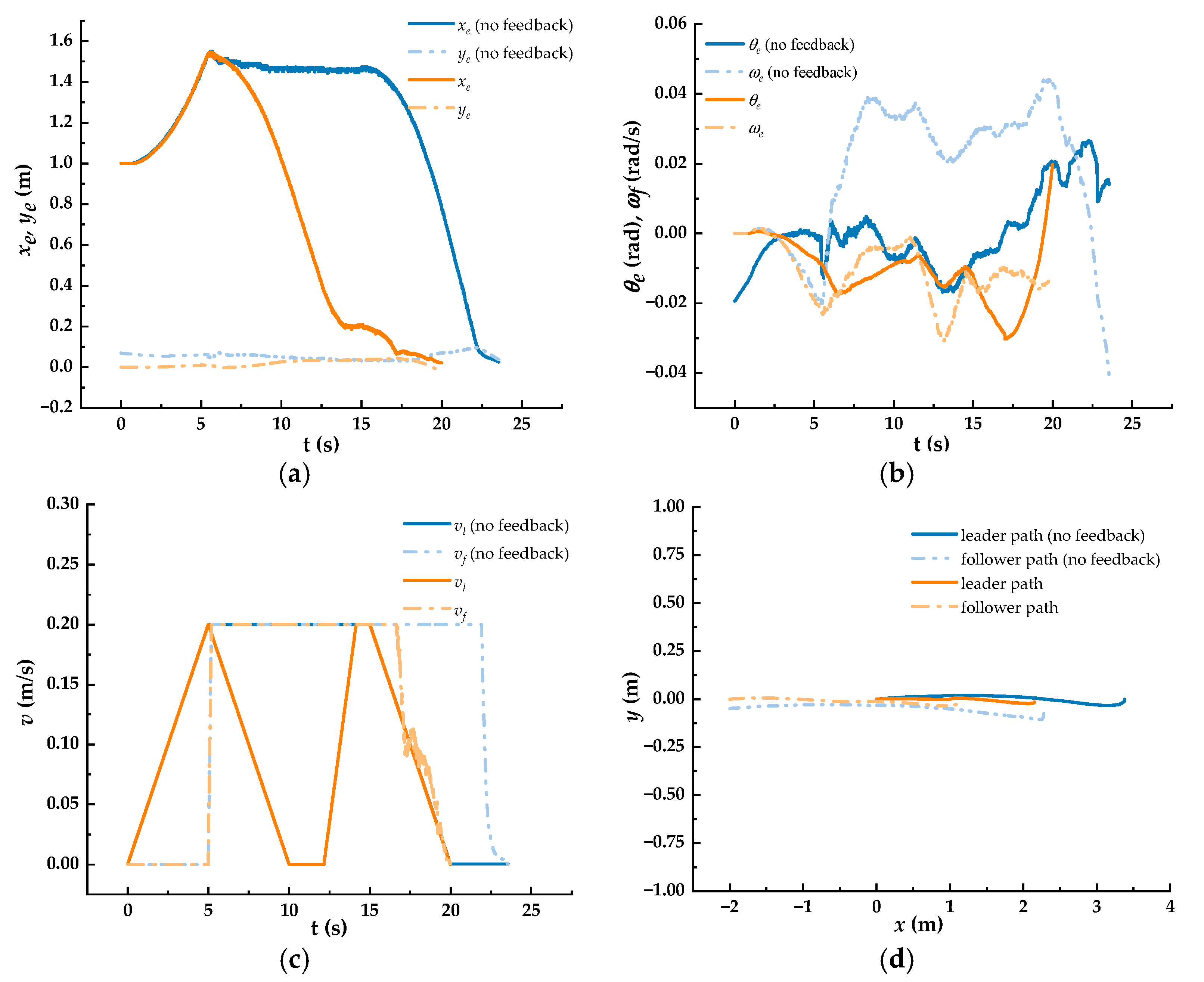
5.1. Simulation with the Formation Feedback Mechanism
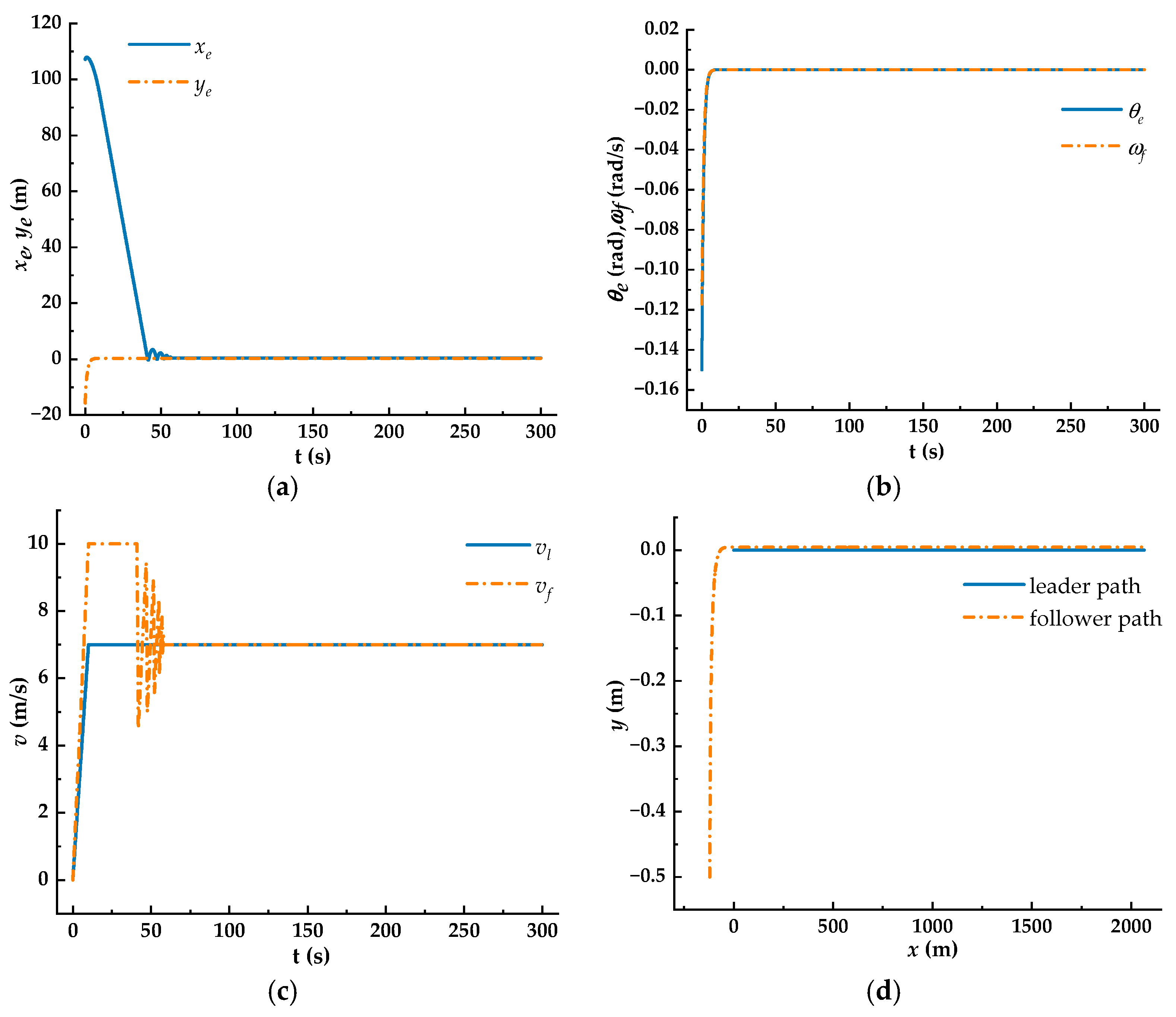
5.2. Simulation with the Dual AGVs’ Form Maintains the Formation
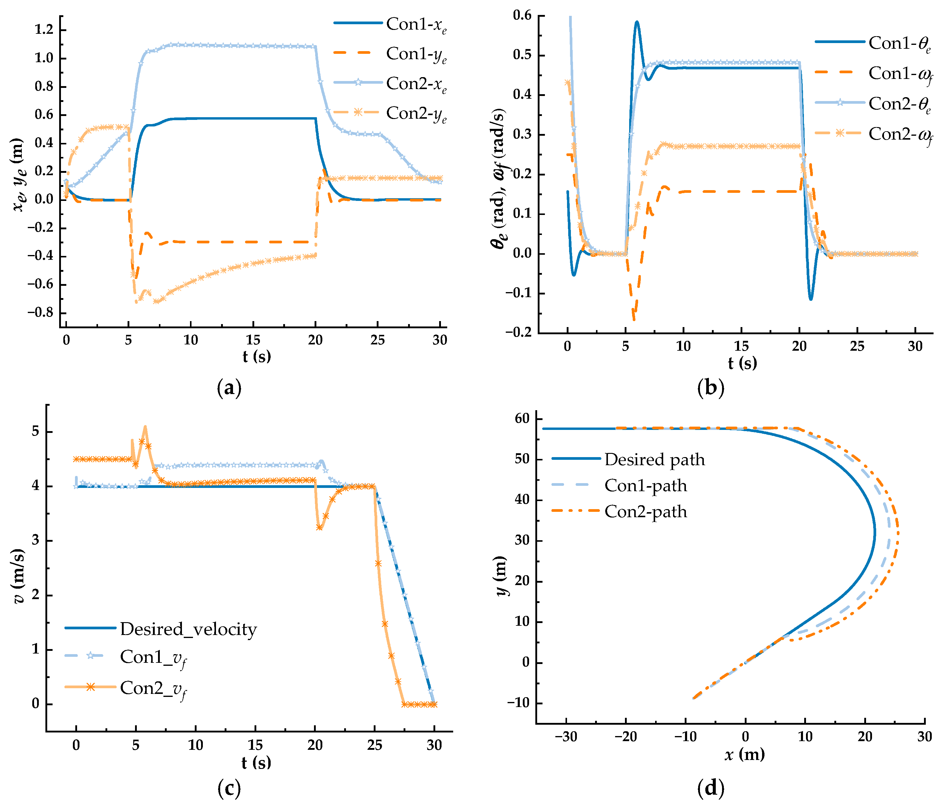
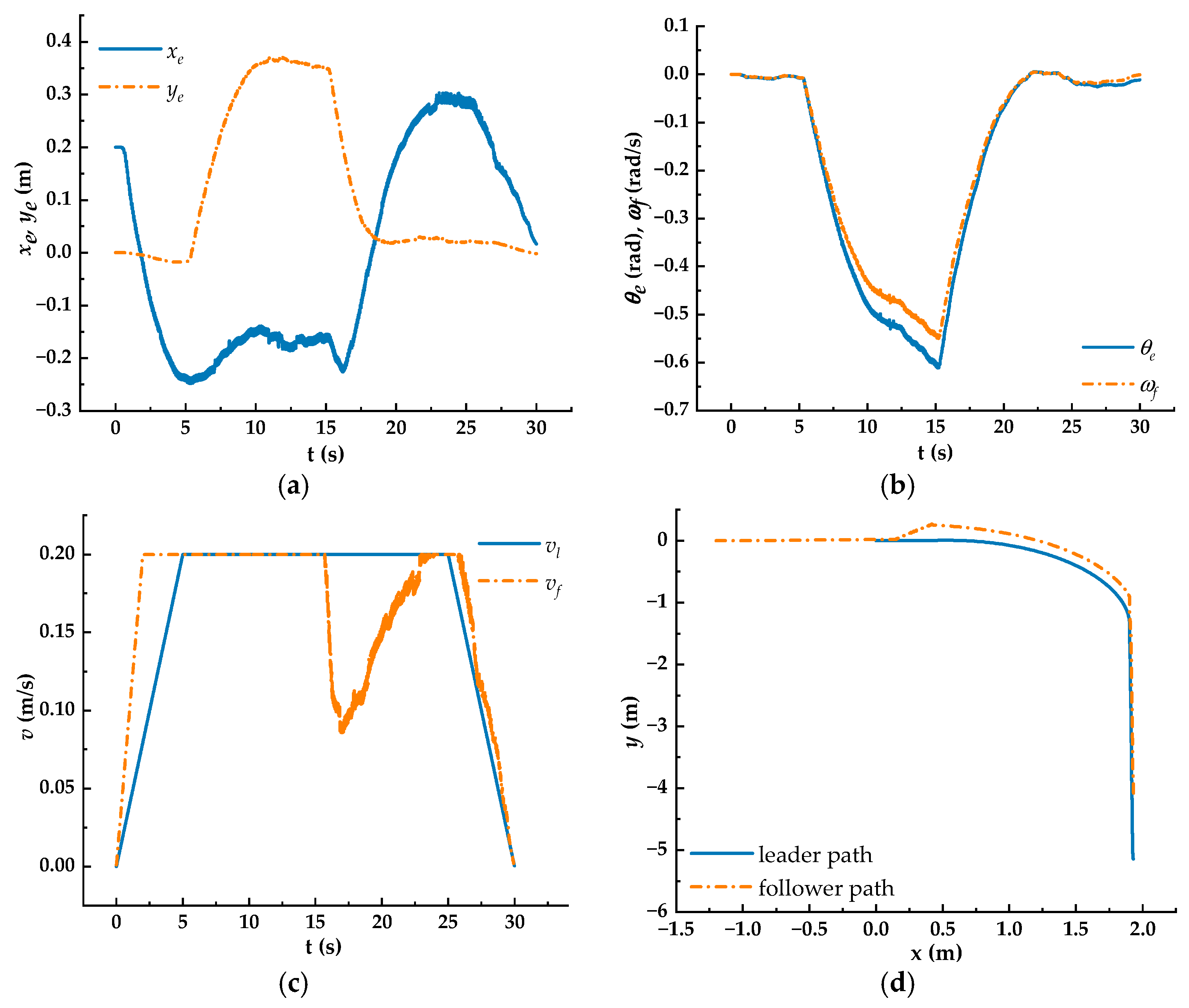
5.3. Simulation in Turning Condition
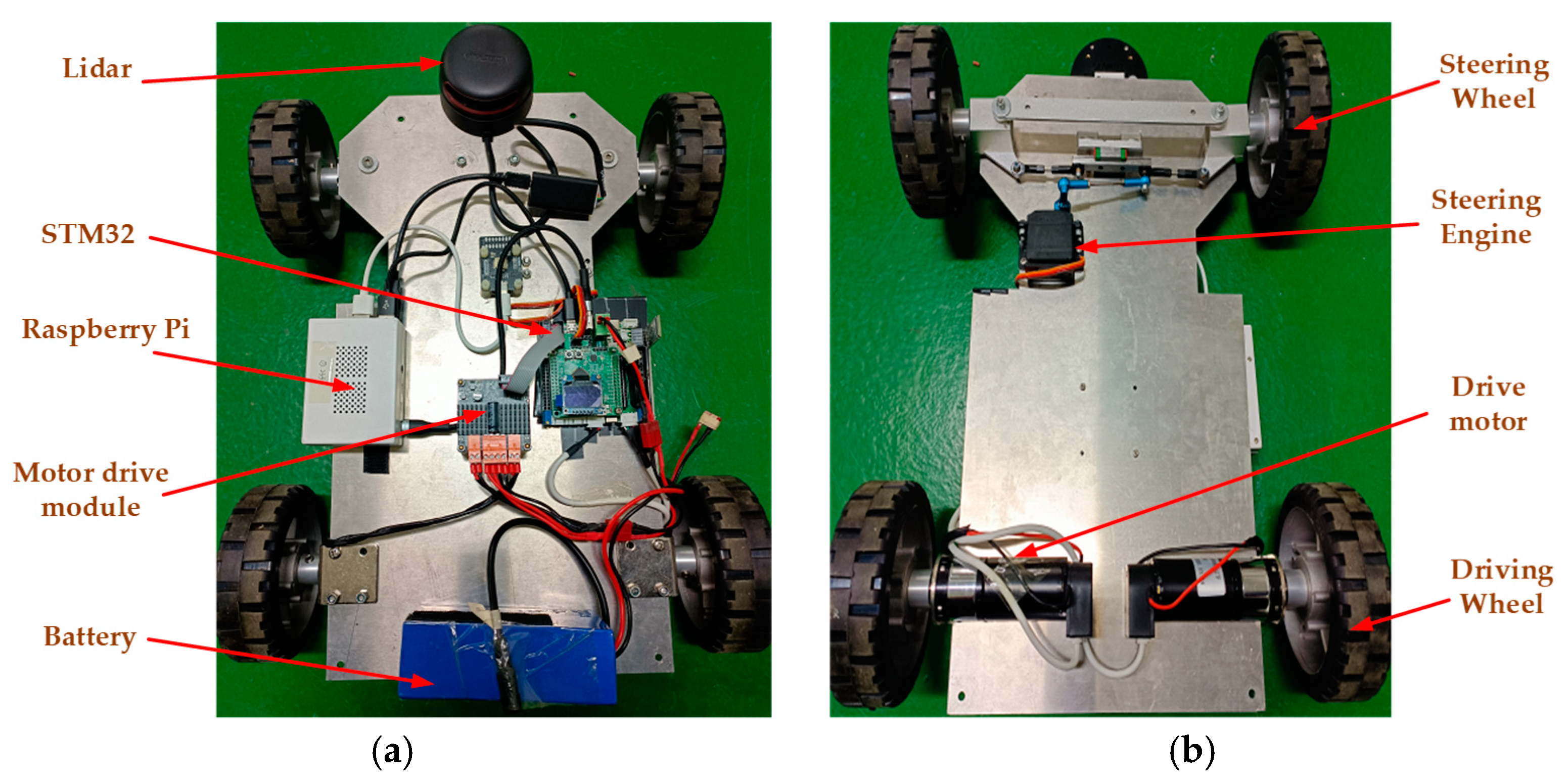
6. Experiments and Analysis
6.1. Experiment with the Formation Feedback Mechanism
6.2. Experiment in Turning Condition
7. Conclusions
Author Contributions
Funding
Institutional Review Board Statement
Informed Consent Statement
Data Availability Statement
Conflicts of Interest
References
- Kon, W.K.; Abdul Rahman, N.S.F.; Md Hanafiah, R.; Abdul Hamid, S. The Global Trends of Automated Container Terminal: A Systematic Literature Review. Marit. Bus. Rev. 2021, 6, 206–233. [Google Scholar] [CrossRef]
- Lau, Y.; Chen, Q.; Poo, M.C.-P.; Ng, A.K.Y.; Ying, C.C. Maritime Transport Resilience: A Systematic Literature Review on the Current State of the Art, Research Agenda and Future Research Directions. Ocean Coast. Manag. 2024, 251, 107086. [Google Scholar] [CrossRef]
- Pjevcevic, D.; Nikolic, M.; Vidic, N.; Vukadinovic, K. Data Envelopment Analysis of AGV Fleet Sizing at a Port Container Terminal. Int. J. Prod. Res. 2017, 55, 4021–4034. [Google Scholar] [CrossRef]
- Zhang, Q.; Li, W.-F.; Zhou, J.-L. No-Load Formation Control of Dual AGVs Based on Container Terminals. In Proceedings of the 2022 IEEE International Conference on Networking, Sensing and Control (ICNSC), Shanghai, China, 15–18 December 2022; IEEE: Piscataway, NJ, USA, 2022; pp. 1–5. [Google Scholar] [CrossRef]
- Rizzo, C.; Lagrana, A.; Serrano, D. GEOMOVE: Detached AGVs for Cooperative Transportation of Large and Heavy Loads in the Aeronautic Industry. In Proceedings of the 2020 IEEE International Conference on Autonomous Robot Systems and Competitions (ICARSC), Ponta Delgada, Portugal, 15–17 April 2020; IEEE: Piscataway, NJ, USA, 2020; pp. 126–133. [Google Scholar] [CrossRef]
- Huzaefa, F.; Liu, Y.-C. Force Distribution and Estimation for Cooperative Transportation Control on Multiple Unmanned Ground Vehicles. IEEE Trans. Cybern. 2023, 53, 1335–1347. [Google Scholar] [CrossRef]
- Flixeder, S.; Glück, T.; Kugi, A. Force-Based Cooperative Handling and Lay-up of Deformable Materials: Mechatronic Design, Modeling, and Control of a Demonstrator. Mechatronics 2017, 47, 246–261. [Google Scholar] [CrossRef]
- Rosenfelder, M.; Ebel, H.; Eberhard, P. Force-Based Organization and Control Scheme for the Non-Prehensile Cooperative Transportation of Objects. Robotica 2024, 42, 611–624. [Google Scholar] [CrossRef]
- Chen, Q.; Sun, Y.; Zhao, M.; Liu, M. Consensus-Based Cooperative Formation Guidance Strategy for Multiparafoil Airdrop Systems. IEEE Trans. Autom. Sci. Eng. 2021, 18, 2175–2184. [Google Scholar] [CrossRef]
- Su, Y.-H.; Bhowmick, P.; Lanzon, A. A Robust Adaptive Formation Control Methodology for Networked Multi-UAV Systems with Applications to Cooperative Payload Transportation. Control Eng. Pract. 2023, 138, 105608. [Google Scholar] [CrossRef]
- Er, M.J.; Li, Z. Formation Control of Unmanned Surface Vehicles Using Fixed-Time Non-Singular Terminal Sliding Mode Strategy. J. Mar. Sci. Eng. 2022, 10, 1308. [Google Scholar] [CrossRef]
- Guo, J.; Liu, Z.; Song, Y.; Yang, C.; Liang, C. Research on Multi-UAV Formation and Semi-Physical Simulation With Virtual Structure. IEEE Access 2023, 11, 126027–126039. [Google Scholar] [CrossRef]
- Wen, J.; Yang, J.; Li, Y.; He, J.; Li, Z.; Song, H. Behavior-Based Formation Control Digital Twin for Multi-AUG in Edge Computing. IEEE Trans. Netw. Sci. Eng. 2023, 10, 2791–2801. [Google Scholar] [CrossRef]
- Chen, F.; Ren, W. Multi-Agent Control: A Graph-Theoretic Perspective. J. Syst. Sci. Complex. 2021, 34, 1973–2002. [Google Scholar] [CrossRef]
- He, S.; Wang, M.; Dai, S.-L.; Luo, F. Leader-Follower Formation Control of USVs With Prescribed Performance and Collision Avoidance. IEEE Trans. Ind. Inform. 2019, 15, 572–581. [Google Scholar] [CrossRef]
- Wang, Y.; Wang, D.; Yang, S.; Shan, M. A Practical Leader-Follower Tracking Control Scheme for Multiple Nonholonomic Mobile Robots in Unknown Obstacle Environments. IEEE Trans. Control Syst. Technol. 2019, 27, 1685–1693. [Google Scholar] [CrossRef]
- Chang, X.; Jiao, J.; Li, Y.; Hong, B. Multi-Consensus Formation Control by Artificial Potential Field Based on Velocity Threshold. Front. Neurosci. 2024, 18, 1367248. [Google Scholar] [CrossRef]
- Ullah, N.; Mehmood, Y.; Aslam, J.; Ali, A.; Iqbal, J. UAVs-UGV Leader-Follower Formation Using Adaptive Non-Singular Terminal Super Twisting Sliding Mode Control. IEEE Access 2021, 9, 74385–74405. [Google Scholar] [CrossRef]
- Jiang, C.; Guo, Y. Incorporating Control Barrier Functions in Distributed Model Predictive Control for Multirobot Coordinated Control. IEEE Trans. Control Netw. Syst. 2024, 11, 547–557. [Google Scholar] [CrossRef]
- Trinh, M.H.; Tran, Q.V.; Vu, D.V.; Nguyen, P.D.; Ahn, H.-S. Robust Tracking Control of Bearing-Constrained Leader-Follower Formation. Automatica 2021, 131, 109733. [Google Scholar] [CrossRef]
- Xuan-Mung, N.; Hong, S.K. Robust Adaptive Formation Control of Quadcopters Based on a Leader-Follower Approach. Int. J. Adv. Robot. Syst. 2019, 16, 172988141986273. [Google Scholar] [CrossRef]
- Liu, X.; Ge, S.S.; Goh, C.-H. Vision-Based Leader-Follower Formation Control of Multiagents With Visibility Constraints. IEEE Trans. Control Syst. Technol. 2019, 27, 1326–1333. [Google Scholar] [CrossRef]
- He, J.; Liao, J. Formation Tracking Control with Disturbance Rejection in Leader-Follower Multi-Agent Systems under Dynamic Event-Triggered Mechanism. Eng. Appl. Artif. Intell. 2024, 133, 108441. [Google Scholar] [CrossRef]
- Khodamipour, G.; Khorashadizadeh, S.; Farshad, M. Adaptive Formation Control of Leader-Follower Mobile Robots Using Reinforcement Learning and the Fourier Series Expansion. ISA Trans. 2023, 138, 63–73. [Google Scholar] [CrossRef] [PubMed]
- Li, M.; Liu, H.; Xie, F.; Huang, H. Adaptive Distributed Control for Leader-Follower Formation Based on a Recurrent SAC Algorithm. Electronics 2024, 13, 3513. [Google Scholar] [CrossRef]
- Gao, Z.; Guo, G. Fixed-Time Leader-Follower Formation Control of Autonomous Underwater Vehicles With Event-Triggered Intermittent Communications. IEEE Access 2018, 6, 27902–27911. [Google Scholar] [CrossRef]
- Wang, Y.; Shan, M.; Yue, Y.; Wang, D. Vision-Based Flexible Leader-Follower Formation Tracking of Multiple Nonholonomic Mobile Robots in Unknown Obstacle Environments. IEEE Trans. Control Syst. Technol. 2020, 28, 1025–1033. [Google Scholar] [CrossRef]
- Li, Z.; Yuan, Y.; Ke, F.; He, W.; Su, C.-Y. Robust Vision-Based Tube Model Predictive Control of Multiple Mobile Robots for Leader-Follower Formation. IEEE Trans. Ind. Electron. 2020, 67, 3096–3106. [Google Scholar] [CrossRef]
- Shen, H.; Yin, Y.; Qian, X. Fixed-Time Formation Control for Unmanned Surface Vehicles with Parametric Uncertainties and Complex Disturbance. J. Mar. Sci. Eng. 2022, 10, 1246. [Google Scholar] [CrossRef]
- Li, K.; Shen, Z.; Jing, G.; Song, Y. Angle-Constrained Formation Control under Directed Non-Triangulated Sensing Graphs. Automatica 2024, 163, 111565. [Google Scholar] [CrossRef]
- Wang, S.; Wang, H.; Li, Y.; Li, Q. Distributed Finite-Time Neuroadaptive Fault-Tolerant Formation Control for Multi-Robot Systems. Appl. Ocean. Res. 2024, 150, 104067. [Google Scholar] [CrossRef]
- Du, Z.; Zhang, H.; Wang, Z.; Yan, H. Model Predictive Formation Tracking-Containment Control for Multi-UAVs With Obstacle Avoidance. IEEE Trans. Syst. Man Cybern. Syst. 2024, 54, 3404–3414. [Google Scholar] [CrossRef]
- Wang, C.; Sun, Y.; Ma, X.; Chen, Q.; Gao, Q.; Liu, X. Multi-Agent Dynamic Formation Interception Control Based on Rigid Graph. Complex Intell. Syst. 2024, 10, 5585–5598. [Google Scholar] [CrossRef]
- Guo, T.; Liu, Y.; Hu, H.-X. Adaptive Connectivity-Preserving Formation Control with a Dynamic Event-Triggering Mechanism. J. Frankl. Inst. 2025, 362, 107331. [Google Scholar] [CrossRef]


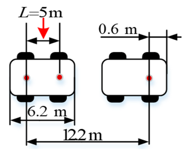
| Specification | 20 ft | 40 ft | 45 ft |
|---|---|---|---|
| Length/m | 6.058 | 12.192 | 13.716 |
| Width/m | 2.438 | 2.438 | 2.438 |
| Height/m | 2.591 | 2.591 | 2.896 |
Disclaimer/Publisher’s Note: The statements, opinions and data contained in all publications are solely those of the individual author(s) and contributor(s) and not of MDPI and/or the editor(s). MDPI and/or the editor(s) disclaim responsibility for any injury to people or property resulting from any ideas, methods, instructions or products referred to in the content. |
© 2025 by the authors. Licensee MDPI, Basel, Switzerland. This article is an open access article distributed under the terms and conditions of the Creative Commons Attribution (CC BY) license (https://creativecommons.org/licenses/by/4.0/).
Share and Cite
Zhang, Q.; Li, W.; Guo, L.; Qi, X. Collaborative Transport Strategy for Dual AGVs in Smart Ports: Enhancing Docking Accuracy in No-Load Formations. J. Mar. Sci. Eng. 2025, 13, 81. https://doi.org/10.3390/jmse13010081
Zhang Q, Li W, Guo L, Qi X. Collaborative Transport Strategy for Dual AGVs in Smart Ports: Enhancing Docking Accuracy in No-Load Formations. Journal of Marine Science and Engineering. 2025; 13(1):81. https://doi.org/10.3390/jmse13010081
Chicago/Turabian StyleZhang, Qiang, Wenfeng Li, Long Guo, and Xiaohang Qi. 2025. "Collaborative Transport Strategy for Dual AGVs in Smart Ports: Enhancing Docking Accuracy in No-Load Formations" Journal of Marine Science and Engineering 13, no. 1: 81. https://doi.org/10.3390/jmse13010081
APA StyleZhang, Q., Li, W., Guo, L., & Qi, X. (2025). Collaborative Transport Strategy for Dual AGVs in Smart Ports: Enhancing Docking Accuracy in No-Load Formations. Journal of Marine Science and Engineering, 13(1), 81. https://doi.org/10.3390/jmse13010081