Abstract
In the coastal zone, two types of habitats—linear and areal—are distinguished. The main differences between both types are their shape and structure and the hydro- and litho-dynamic, salinity, and ecological gradients. Studying linear littoral habitats is essential for interpreting the ’coastal squeeze’ effect. The study’s main objective was to assess short-term behavior of soft cliffs as littoral linear habitats during calm season storm events in the example of the Olandų Kepurė cliff, located on a peri-urban protected seashore (Baltic Sea, Lithuania). The approach combined the surveillance of the cliff using unmanned aerial vehicles (UAVs) with the data analysis using an ArcGIS algorithm specially adjusted for linear habitats. The authors discerned two short-term behavior forms—cliff base cavities and scarp slumps. The scarp slumps are more widely spread. It is particularly noticeable at the beginning of the spring–summer period when the difference between the occurrence of both forms is 3.5 times. In contrast, cliff base cavities proliferate in spring. This phenomenon might be related to a seasonal Baltic Sea level rise. The main conclusion is that 55 m long cliff cells are optimal for analyzing short-term cliff behavior using UAV and GIS.
1. Introduction
Two types of littoral habitats should be distinguished in the coastal zone—linear and areal. The concept of linear littoral habitats, first proposed by Robles-Diaz-de-León and Nava-Tudela [1] and developed by the coastal research team at Klaipeda University, Lithuania [2,3,4,5], has garnered significant international interest in recent years. It has been applied by a worldwide coastal research community on various coastal management aspects—from coastal dune conservation [6] to coastal forest [7] and fishery management [8].
Referring to the broader international context and relevance of this research study, the main postulate of the concept of linear littoral habitats is about the fundamental morphological and ecological differences that distinguish them from areal habitats. This contrast is an essential research tenet. The main features of the linear coastal habitats are the following:
- Shape: Linear littoral habitats are narrow habitats characterized by a vast longitudinal range compared to a relatively thin width.
- Structure: Linear littoral habitats are relatively homogenous. It contrasts with areal littoral habitats, which are typically patchy.
- Distinctive gradients: The boundaries of linear littoral habitats are defined by steep and distinctive hydro- and litho-dynamic, salinity, and ecological gradients, which feature the complexity of these ecosystems.
Understanding linear littoral habitats is vital for responding to problems such as the ‘coastal squeeze’ effect in modern coastal evolution [9]. Pontee [10], p. 206, defines coastal squeeze as one form of coastal habitat loss, where intertidal habitat is lost due to the high-water mark being fixed by a defense or structure (…) and the low-water mark migrating landwards in response to sea level rise. It threatens the integrity of linear littoral habitats by breaking and fragmenting these narrow, long-shore strips. It is acute, where artificial consolidation on the coastline affects habitats and ecosystems that typically retreat landward due to coastal erosion [11,12].
The growing tourism pressure on linear littoral habitats causes coastal development for urban sprawl, tourism, recreation, and industry [13]. Narrow sandy beaches are particularly vulnerable and threatened to disappear due to coastal squeeze [14]. Sandy coasts are highly developed and densely populated due to their recreational amenities and visual appeal. Erosion of these coasts over the last few decades has already resulted in coastal squeeze [10,15]. This study focuses not on soft cliff erosion per se but on a broader, comprehensive consideration of cliff behavior in peri-urban protected shorelines, which simultaneously are attractive tourist destinations [16,17].
In 2022, the authors of the present study investigated current main trends in two interrelated complex research fields pertinent to the objectives of the study: (i) biodiversity conservation and tourism sustainability [18], and (ii) applications of remote sensing for coastal and marine nature conservation [19]. By applying hierarchical cluster analysis with a KH Coder 3.0 tool, major trending research themes on biodiversity conservation and tourism sustainability were identified, including community-based tourism development [20,21,22], national park management for tourism [23,24,25], sustainable tourist motivation [26,27,28], and biodiversity conservation and ecotourism [29,30,31].
Similarly, using the same technique, four trending research themes in applications of remote sensing in coastal and marine conservation were identified, including remote sensing-based classification and modelling [32,33,34], conservation of tropical coastal and marine habitats [35,36,37], mapping of habitats and species distribution [38,39,40], and ecosystem and biodiversity conservation and resource management [41,42,43]. The objectives of our study stem directly from the above findings as summing up the identified key research directions; joining the application of unmanned aerial vehicle (UAV) imagery with GIS for monitoring coastal habitats in protected areas emerges as one of the resulting pivotal research directions.
The central insight is an increasing coastal habitat vulnerability resulting from growing external impacts like climate change and sea level rise. Thus, if a littoral linear habitat happens to be an attractive peri-urban beach or a soft cliff prone to the combined adverse effects of the urban sprawl, sea level rise and coastal squeeze, coastal managers risk appearing in a ‘perfect storm’ situation regarding coastal cliff behavior. In this situation, the ad hoc flexible application of UAVs owned by coastal managers is convenient for vulnerable littoral habitat monitoring [44].
Furthermore, ArcGIS is a convenient spatial interpretation toolbox available at many coastal conservation and management institutions. Therefore, our study aimed to test the capabilities of the combined use of UAV imagery and ArcGIS to survey and interpret the behavior of linear littoral habitats that are popular tourist attractions in the calm seasons of the year. Olandų Kepurė is a typical soft cliff, i.e., ‘formed through the exposure of rocks that have little resistance’ [45] p. 2, in this case, deposits of glacial till and sandy clay. It is well suited to investigate and understand the behavior of linear littoral habitats under complex stress and its implications for coastal management.
Although the application of UAVs is limited for monitoring in wide and long coastal zones due to stability issues and other technical limitations, for a narrow, ca. 50 m wide, 1.5 km long stretch of a linear littoral habitat like Olandų Kepurė, it is more flexible to study short-term behavior than using satellite data. Hence, we hypothesized that it is possible to study the short-term behavior of the soft cliff as a linear littoral habitat if sufficient precision of remote sensing is achieved and a 1-D interpretation using ArcGIS is applied.
2. Materials and Methods
2.1. Study Area
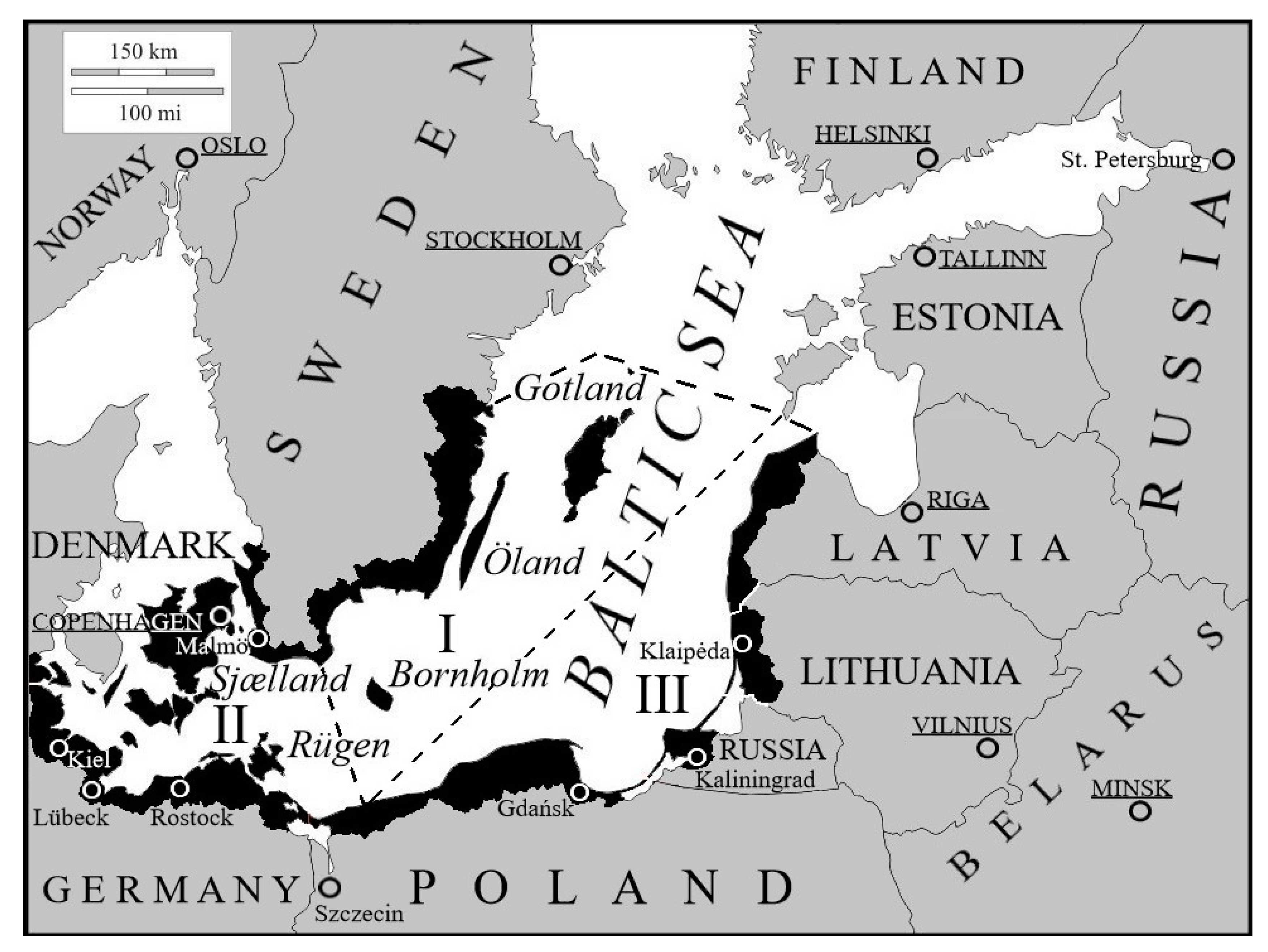
Considering the diversity of South Baltic coastal habitats and patterns of seaside recreational resources, the South Baltic coastal region can be divided into three sub-regions (Figure 1):

Figure 1.
South Baltic Seaside Region: I—Southeast Scandinavian coast and islands; II—South Baltic coast and islands; III—Southeast Baltic graded coast.
- Southeast Scandinavian coast and islands;
- South Baltic coast and islands;
- Southeast Baltic graded coast.
The morphological and habitat features of the Southeast Baltic graded coast resulted from the post-glacial Baltic Sea level fluctuations combined with the sediment input from large rivers, erosion of moraine promontories, and a longshore marine sediment drift [46]. Here, the graded coast is defined as the one where the headland erosion and deposition of eroded sediments in adjacent embayments grades the shoreline configuration in the long term [47]. Our study area is one of such Southeast Baltic coastal features—the highest sea cliff in Lithuania—Olandų Kepurė, ca. 25 m high at the highest point. Its annual erosion rate ranges from 0.5 m to 2.2 m.
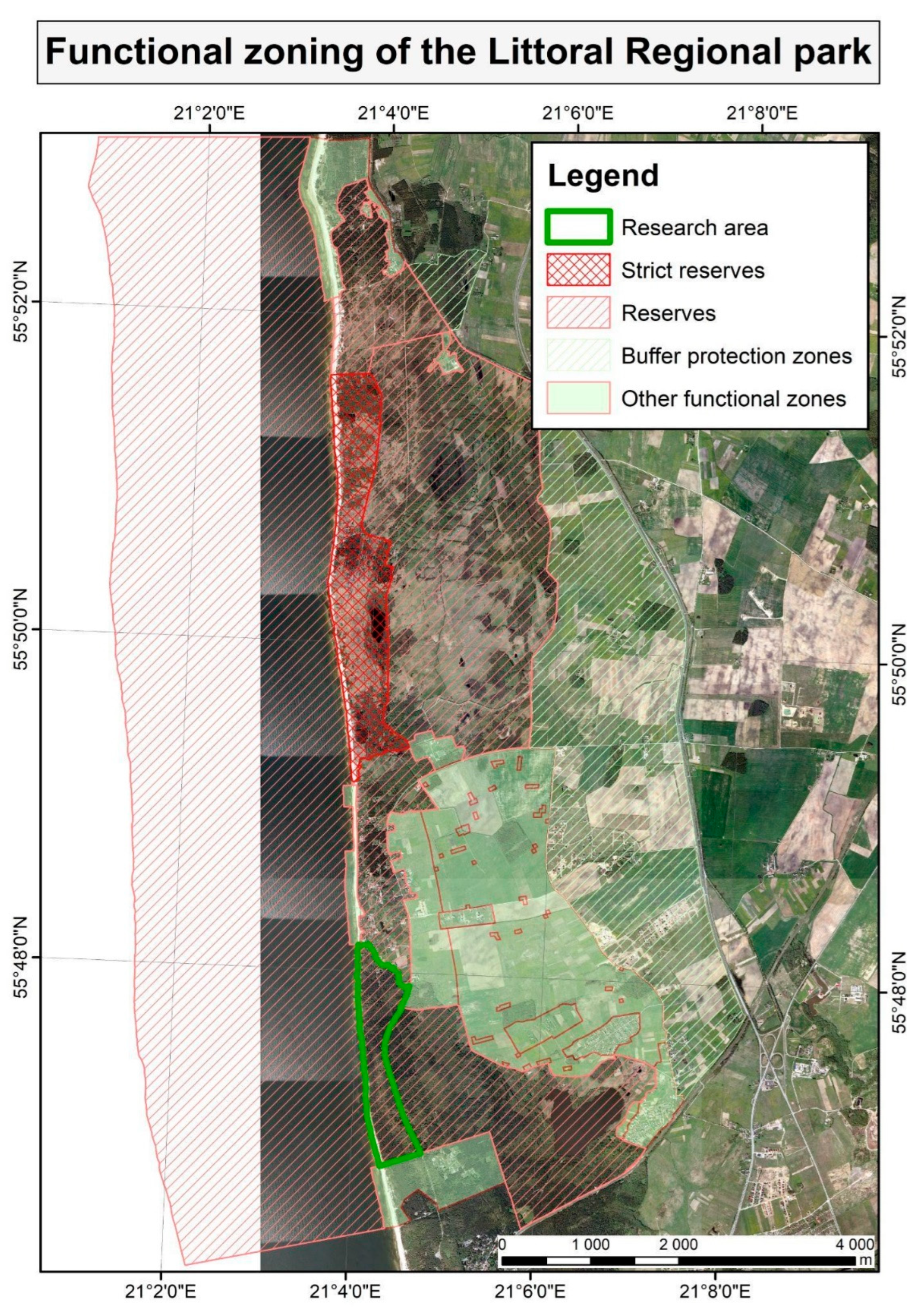
The Olandų Kepurė sea cliff is protected as a landscape reserve within an IUCN category V peri-urban Littoral Regional Park (Figure 2). It is a littoral linear mega-habitat comprising a shoreline-parallel series of the underwater boulder belt, nearshore sand belt, gravel strip, sand beach, cliff base and cliff slope (Figure 3). The areal part of the Olandų Kepurė landscape reserve includes several habitats related to the prevailing mature, up to 120-year-old Scots’ pine forests of a local Eastern Baltic race (Pinus sylvestris var. rigensis Loudon). Also, over 200-year-old English oak (Quercus robur) trees and over 120-year-old Norway spruce (Picea abies) trees grow in the Olandų Kepurė nature reserve, constituting its landscape and ecosystem value [48].
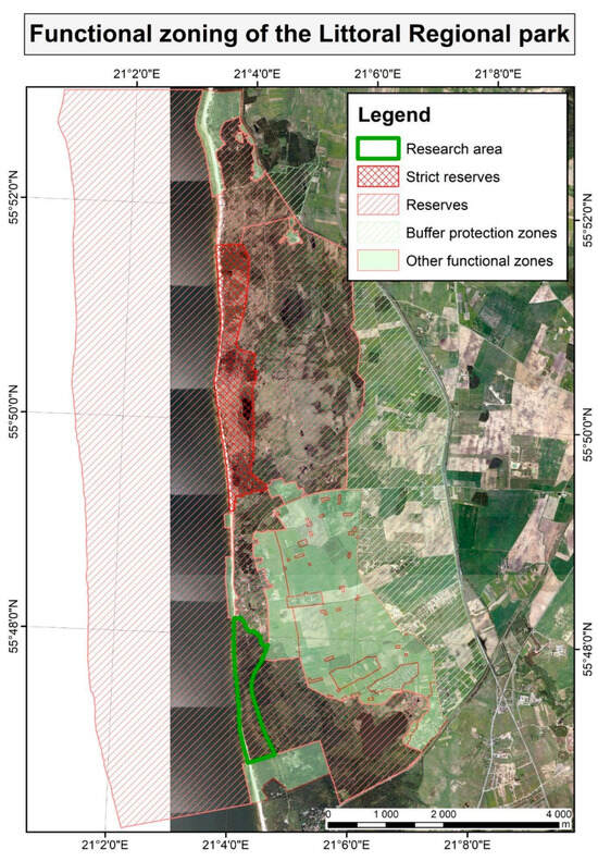
Figure 2.
GIS map of functional zoning of the Littoral Regional Park. The delimitation of the Olandų Kepurė landscape reserve is marked with a green line.

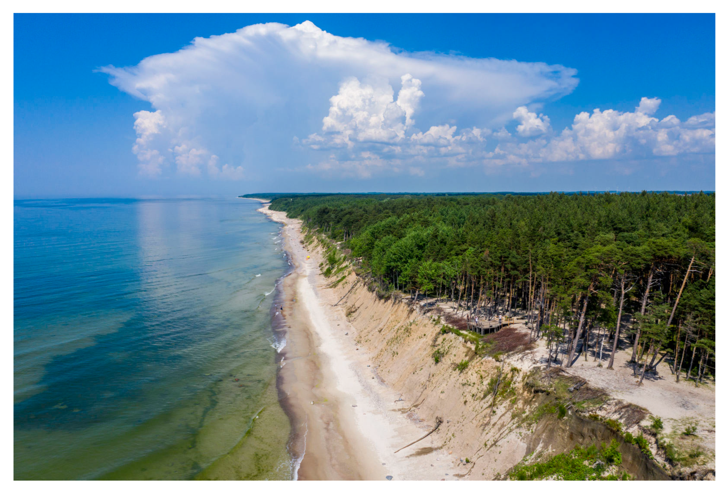
Figure 3.
The Olandų Kepurė sea cliff with a longshore series of linear littoral habitats (from left to right): underwater boulder belt, nearshore sand belt, gravel strip, sand beach, cliff base, cliff slope. (Credit: Administration of Lithuania Minor Protected Areas).
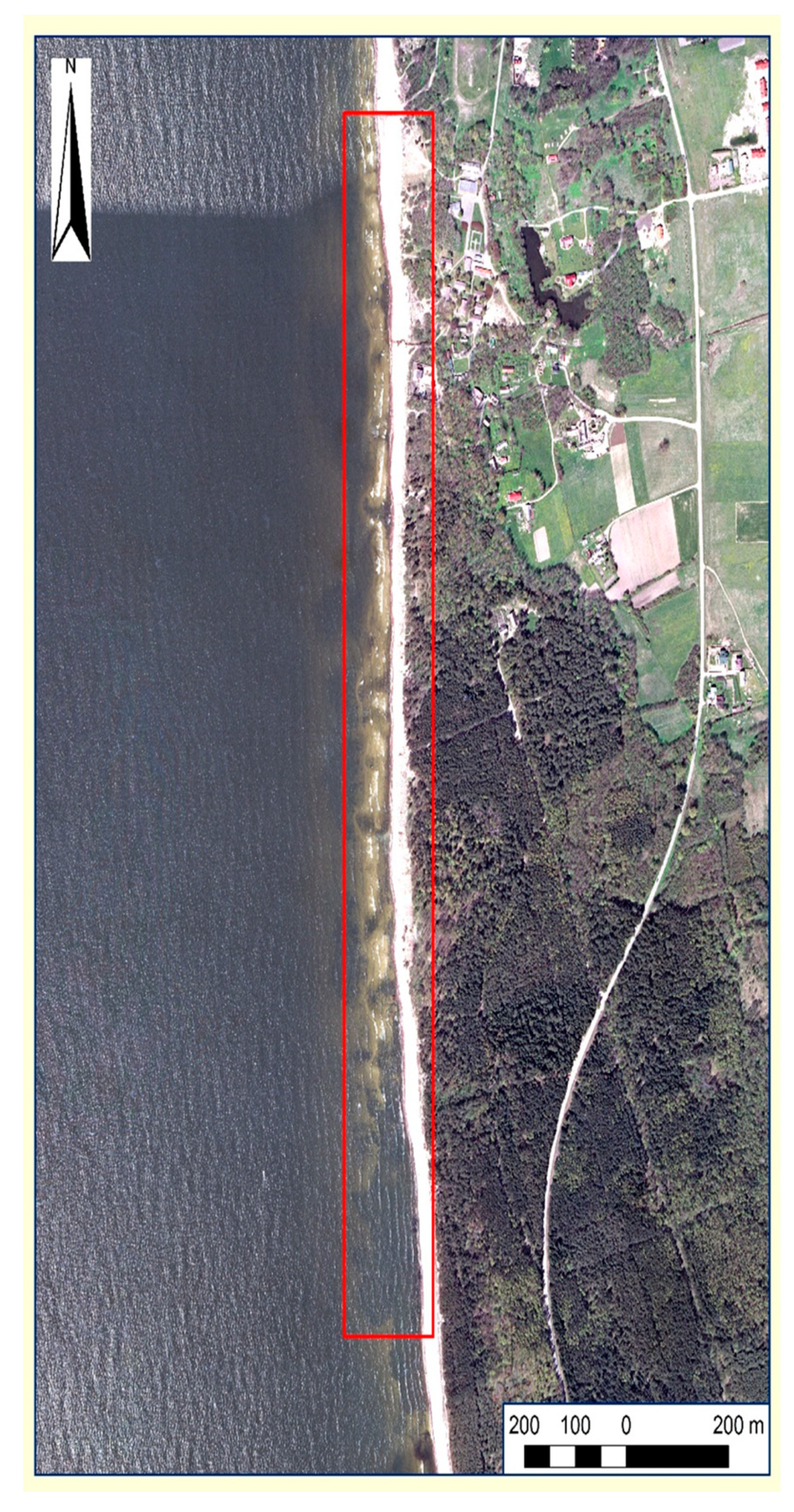
The Olandų Kepurė sea cliff is a 1.5 km long stretch of the Baltic Sea coast north of Klaipeda, the third-largest urban agglomeration of Lithuania (Figure 4). It is the most popular single-day outdoor active visitor attraction on the Lithuanian Baltic Sea coast. A total of 0.4 million visitors annually visit the cliff. One of the essential management tasks of the Olandų Kepurė landscape reserve is to optimize tourism infrastructure to allow visitors to enjoy the park’s natural and cultural heritage values combined with coastal and maritime tourism. Therefore, it is necessary to investigate the cliff behavior in the relatively calm seasons more appealing to visitors.

Figure 4.
The Olandų Kepurė sea cliff. The study area is within the rectangle with red borders.
Here, we define the calm season as a protracted period of the year when the probability of strong winds with an average wind speed over 20 m/s is below 10% [49], and weather conditions at the Olandų Kepurė cliff are formed predominantly by breeze circulation [50]. The calm season in the South Baltic Region is usually between April and August [51], but it varies from year to year. Respectively, calm season storm events are periods with a wind speed over 20 m/s lasting for one week in the calm season related to North Atlantic cyclones originating in the east Atlantic and passing over the southeast Baltic coast [52].
According to the information from the Ranger’s Office of the Littoral Regional Park [53], the climate features of the Olandų Kepurė landscape reserve in the current climatic standard norm period (1991 to 2020) are typical for a temperate Atlantic climate coastal region featured by mild winters, more clear days, more frequent thunderstorms. The annual number of cloudy days is 98 to 111 days per year. About 100 sunny days occur in the warm season (i.e., May–September). The average annual precipitation rate is 696 mm, of which 63% falls in the warm season (April to October).
The average air temperature ranges from +5 °C to +12 °C in spring, + 14 °C to + 17 °C in summer, +12.5 °C to +5 °C in autumn and −4 °C to −1 °C in winter. The Baltic Sea tidal range at Olandų Kepurė is 3.5 cm. Prevailing SW and SE air masses shape the dynamic conditions in the Baltic Sea nearshore. The Olandų Kepurė cliff is exposed to the longest fetches of the severest autumn and winter storms and wave directions (SW, W and NW). The range of the seasonal change in the water level of the Baltic Sea caused by the wind is 22 cm to 28 cm.
2.2. Research Overview
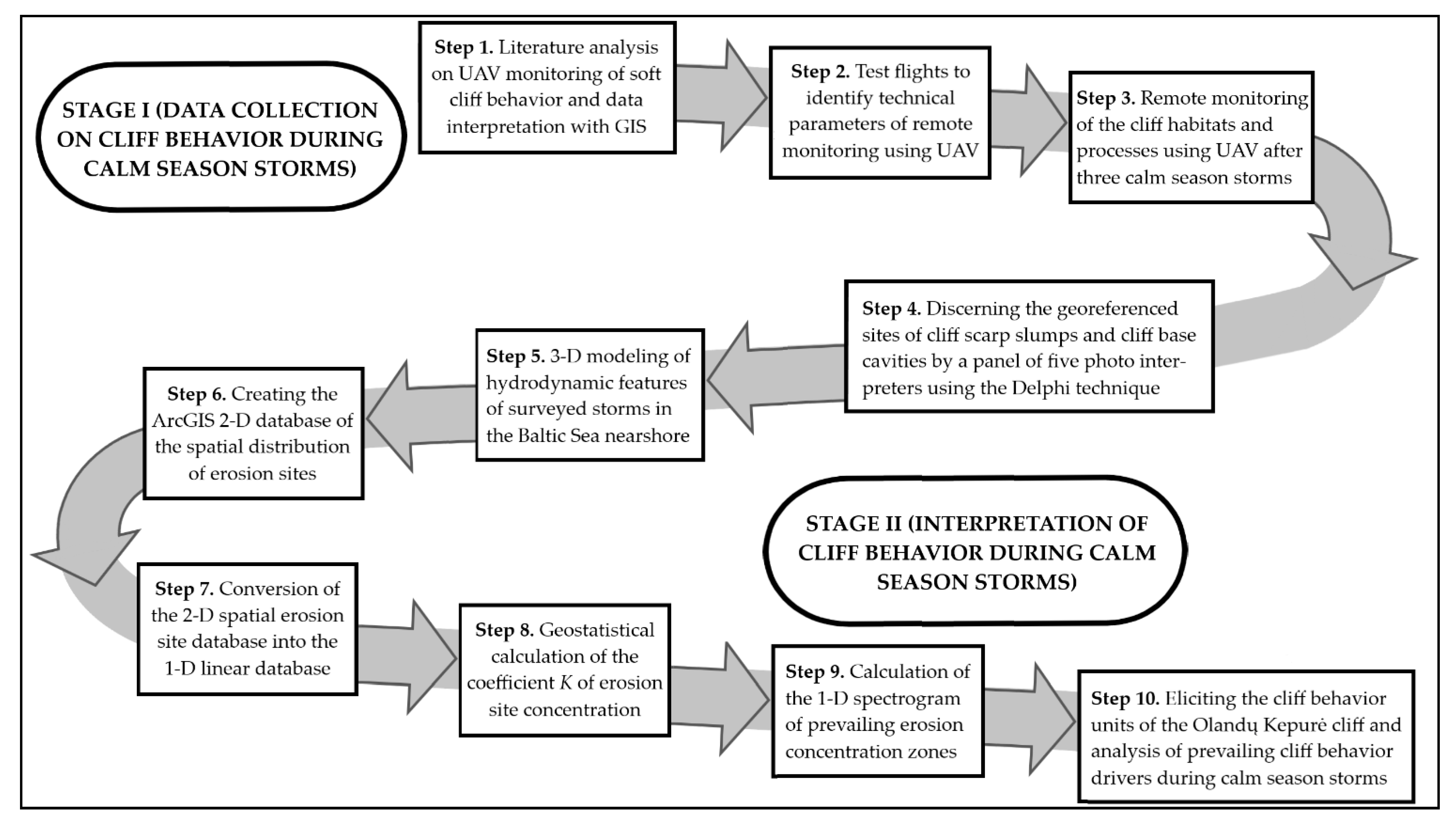
Figure 5 summarizes the research methodology, workflow, and the interrelation of steps. The assessment of cliff behavior along the entire 1.5 km length of the Olandų Kepurė sea cliff during the calm season storm events used a blend of qualitative and quantitative methods, resulting in a mixed technique proven productive in other coastal GIS-based studies [54,55,56,57,58,59]. The methodology involved pilot cliff monitoring using UAV and data analysis using an ArcGIS algorithm adjusted for linear habitats, accompanied by modelling waves and currents in the storm events before the remote surveillance sessions and the Delphi procedure for identifying the sites of cliff scarp slumps and cliff base cavities.

Figure 5.
The workflow chart of stages and steps of the whole research project.
The pilot cliff monitoring using UAV was for collecting the visual database of the georeferenced sites of the erosion sites. The aim of this pilot monitoring stems from the overall study goal to test if UAVs can be applied for coastal monitoring in a peri-urban protected area, which is a popular tourist destination. The challenge of data input was to optimize the flight parameters for collecting the database of the discernable images of cliff scarp slumps and base cavities. The essential aspect of data output was the visual assessment of taken images regarding resolution, the area covered, and the detail of objects in the image.
As the database of erosion sites was too small to train the AI visual recognition models for discerning the cliff scarp slumps and cliff base cavities, the authors employed professional photo interpreters for this task using the Delphi technique. It is a reliable method to help reach expert consensus, especially in fuzzy situations. It has been successfully applied worldwide, including by the authors of this study [60]. The initial data input was over 400 UAV-made images provided by the organizer to the panelists as the visual priors. The data output was a georeferenced database of cliff base cavities and scarp slumps, which experts discerned with an 80% consensus.
Since there are no buoys or other hydrodynamic monitoring gauges in the vicinity of Olandų Kepurė, the next step was to apply hydrodynamic modelling to obtain data on water circulation, waves, and water level during the investigated storm events. The 3-D simulation model was applied to simulate and understand spatiotemporal hydrodynamics of the Baltic Sea near the Olandų Kepurė cliff during three investigated storm events. The input data were obtained from the Klaipeda Maritime Observatory, and the output data were simulated hourly hydrodynamic parameters at Olandų Kepurė during three storm events (25 February–3 March 2023, 1–7 April 2023, and 18–24 August 2023).
The final step of this study was to apply a Geographic Information System (GIS) to interpret the spatial distribution of the cliff scarp slumps and base cavities, thereby determining their distribution’s essential patterns. As academic literature highlights, GIS offers many coastal monitoring and conservation benefits [61,62,63,64]. This study applied the GIS software ArcGIS10.8® by ESRITM (Redlands, CA, USA) to determine the short-term spatial distribution patterns and changes in sea cliff behavior. The input data were quarried from the georeferenced database of the spatial distribution of the discerned erosion sites after each of the three surveyed storm events. The application of GIS by geostatistical analysis enabled discerning the concentration zones of the erosion sites along the cliff’s length.
2.3. Monitoring Using UAV
A UAV Phantom 3 Professional was used, which supports GPS geolocation and is equipped with a Sony EXMOR 1/2.3” camera with a resolution of 12.76 million pixels. The first stage of the image collection included three test flights (on 22 February 2023—twice, and on 27 February 2023) at altitudes of 70 m, 40 m, and 25 m. The objective of the test flights was to find the optimal flight parameters that would be most suitable for collecting the database of the cliff images. The chosen strategy was to start flying from an altitude of 70 m, gradually reducing it to 40 m and 25 m.
The chosen strategy was to start flying from an altitude of 70 m, gradually reducing it to 40 m and 25 m. Since the Olandų Kepurė cliff height reaches 25 m, the minimum flight height of 25 m was reasonable. During each test flight, at least 25 test images were taken. We further assessed the visual quality of the obtained images. Considering that cliff scarp slumps and base cavities might be 1 m in diameter, it was decided to use the flight height of 25 m for further image database collection. The visual wavelength spectrum was applied in the UAV surveillance. We conducted the surveillance flights to collect the image database after the storm events on 3 March 2023, 7 April 2023, and 24 August 2023.
2.4. Delphi Technique
A group of five experts in coastal geomorphology, coastal management, integrated coastal and maritime planning, and coastal conservation, with good knowledge of soft cliffs and who did not interact directly with each other, accomplished the Delphi study by achieving consensus judgment. There is no single opinion regarding the optimal number of panelists in the Delphi method [65], with heterogeneity being an essential factor in eliciting reliable responses [66]. In a systematic review of Delphi studies, Boulkedid et al. [66] found the minimum number of panelists to be three.
First, the experts were introduced to the proposed method of the coastal erosion site, discerning from the UAV-made images and the possible variety of the visual shapes of cliff base cavities and scarp slumps. Then, experts were asked to discern the cliff base cavities and scarp slumps in the images. Next, the organizer collected, summarized, and returned the first judgments to the panelists for further evaluation. These judgments included the responses of other panelists, allowing each expert to scrutinize the opinions of others and adjust their own. In the next two rounds, the study organizer sent the revised judgments, with feedback from other panelists, back to the experts.
For this study, the experts performed three rounds of judgment using an approach drawn from previous Delphi studies in landscape management found in the literature [67,68,69,70,71,72,73,74]. The Delphi study was carried out from February to May 2024 using e-mail for communication within the panel of five experts. During the feedback, there was an apparent tendency among the panelists to converge their opinions and seek a consensus. Thus, the research team successfully narrowed the experts’ judgments. After the third round, the respondents reached a satisfactory consensus of 80% of their opinions regarding the discerning of the cliff scarp slumps and cliff base cavities.
2.5. Nearshore Wave Height, Surge Level and Longshore Current Modelling
We employed a 3-D Shallow water HYdrodynamic Finite Element Model SHYFEM [75], an open-source hydrodynamic modelling platform (http://www.ismar.cnr.it/shyfem, accessed on 1 October 2024), to simulate the hydrodynamic parameters. SHYFEM was developed at CNR-ISMAR, a marine research institute in Venice and successfully applied to many shallow water environments [76,77,78,79,80,81,82,83,84,85]. SHYFEM simulates physical variables, such as water circulation, waves, water level, and temperature, necessary to characterize the shallow water spatiotemporal dynamics, and resolves shallow water hydrodynamic equations for lagoons, coastal seas, estuaries, and lakes. The model uses an unstructured grid (finite elements) to discretize the studied spatial aquatic domain. The finite elements are essential in simulating nearshore hydrodynamics [85].
These finite elements allow for the model’s better adaptation to the system’s morphology and bathymetry, ensuring a more accurate representation of real-world conditions [82]. A detailed description of the model and illustrations of its 2-D and 3-D applications can be found in [82,83,84]. The model calculated sea levels, wave heights, longshore current direction, and speed for these periods in the Baltic Sea nearshore up to a 20 m depth contour varying from 250 m at Olandų Kepurė to 10 km in the Baltic Proper. The atmospheric forcing was interpolated from a regular regional climate model data grid into the finite-element nodes by bi-linear interpolation using the algorithm outlined in [85].
2.6. Application of GIS
ArcGIS 10.8® by ESRITM was chosen since it has proved to be an efficient toolbox for versatile analytical purposes [64,86,87,88,89,90]. However, our purpose was quite specific: to investigate the behavior patterns of linear littoral habitats. For this purpose, two key assumptions were made. (1) For spatial analysis, linear littoral habitats with a considerable ratio of length to width can be treated as linear objects, and (2) the main results of the study can be represented in a 1-D coordinate system without considering the curvatures of the linear object. Using linear planimetry for GIS applications in soil erosion management and coastal planning is a new field of geomorphological and geographical studies [91,92,93].
Nevertheless, creating a 1-D georeferenced linear planimetry is challenging, considering linear littoral habitats’ spatial curvature and gradients. Therefore, the next step was to establish a georeferenced database of the erosion sites along the 1.5 km long Olandų Kepurė cliff using ArcGIS 10.8. The 2-D spatial data were converted into the 1-D georeferenced linear data using our original interpretation algorithm based on the sequence of applying several ArcGIS tools, considering the linear distribution of coastal erosion. We developed the algorithm to extract intended 1-D data using ArcGIS 10.8 Toolkit functions of Points to Line, Generate Points Along Lines, Split Line at Point, Spatial Join, and Snap.
Lastly, using the Attribute Table option in ArcGIS 10.8, the data were exported into a Microsoft Excel format and later used to perform additional calculations. In this way, a GIS database of the research sectors of the Olandų Kepurė cliff was created, which contains information about the center points of coastal erosion processes and their localization. Finally, standard ArcGIS geostatistical tools were applied to interpret the results of our investigation. For this purpose, we calculated the erosion site concentration coefficient K using a standard ArcGIS geospatial analysis tool, Point Density, adapted from 2-D to 1-D structure analysis. It indicates how many erosion sites are present in each cliff cell.
3. Results
3.1. Spatial Behavior Patterns of the Olandų Kepurė Cliff
A ‘cliff scarp slump’ is a cliff erosion case occurring when a coherent bulk of unconsolidated sediments moves down a slope for a short distance [45,94]. The term ‘cliff base cavity’ defines the coastal erosion case in which the hydraulic action of waves during a storm surge forms concave basal hollows of various sizes and duration [95,96,97]. The cliff base is a fuzzy, dynamic interface between the cliff surface and the foreshore [45].
In total, 662 cliff scarp slumps and 348 cliff base cavities were identified in all the investigated cases after three calm season storm events (Figure 6). The geostatistical analysis made it possible to distinguish the concentration zones of the erosion sites along the length of the Olandų Kepurė cliff. For this aim, the erosion site concentration coefficient K was calculated using the standard ArcGIS geospatial analysis tool Point density adapted from 2-D to 1-D structure analysis. It shows how many erosion sites are present in different cells when assessing the condition of various cliff cells.
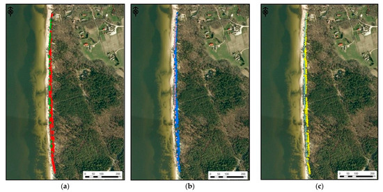
Figure 6.
Distribution of the Olandų Kepurė cliff scarp slumps and base cavities during three UAV flights: (a) 3 March 2023 (slumps in red dots, cavities in green dots); (b) 7 April 2023 (slumps in blue dots, cavities in pink dots); (c) 24 August 2023 (slumps in yellow dots, cavities in white dots).
Figure 6 shows that in all three investigated cases, the cliff scarp slumps occurred relatively evenly along the entire length of the investigated coastline. At the same time, the cliff base cavities were more concentrated in the northern part of the coastline. It can also be seen that in all three cases, the locations of cliff scarp slumps and base cavities and their distribution over the surveyed calm season are unrelated. If erosion occurred in different cases at some sites of the cliff base, then the geographical distribution or intensity of the cliff scarp slumps did not depend on this at all.
The increase in erosion in the northern part of the cliff, rather than with the distribution of slumps, correlates with the intensification of the long-term retreat of the cliff from south to north. In 1954–2003, the previously stable cliff in the northern part of the Olandų Kepurė section retreated by ca. 30 m to 50 m, i.e., 0.6 m to 1 m per year [48]. Meanwhile, at the highest central section of the cliff, the shoreline retreat remained minimal. The intensification of cliff base erosion and long-term shoreline retreat from south to north is associated with the predominance of more erosion-resistant moraine deposits and their large volume in the highest (up to 25 m high) central part of the cliff.
3.2. Spatial Patterns of the Cliff Scarp Slump Distribution
A cliff scarp slump is a common form of mass wasting when loose sediments lie above more cohesive layers such as glacial till, like in the case of the Olandų Kepurė cliff. However, because of their small scale (typically up to 10 m in length and up to 150 m3 in mass) and their ephemeralness, it would be better to label the slumps of the Olandų Kepurė cliff as micro-slumps (Figure 7).
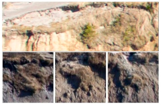
Figure 7.
Examples of the Olandų Kepurė cliff scarp slumps (frontal view taken by a UAV).
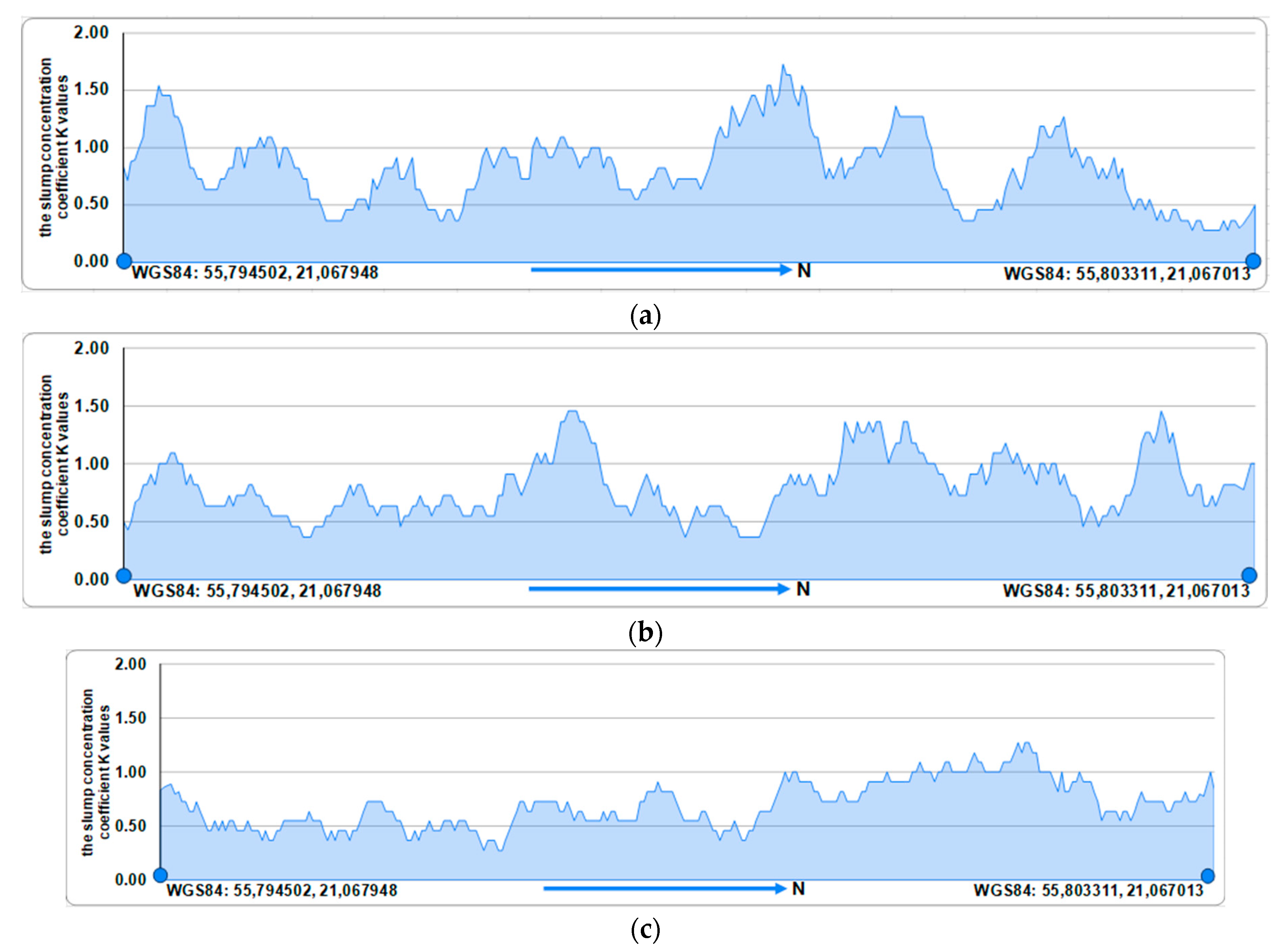
Despite the visually ostensible, quite regular spatial distribution pattern apparent in Figure 6, the distribution of slumps in the study area is far from uniform. The erosion site concentration coefficient K, describing the occurrence of slumps along the Olandų Kepurė cliff scarp, varies significantly, ranging from 0.27 to 1.73 (Figure 8). Regardless of the season, the spatial distribution of slumps along the Olandų Kepurė cliff scarp is very uneven—several investigated cells in the north (on the right in Figure 8), where the cliff is the lowest, feature only a few slumps, i.e., K was equal to 0.27.
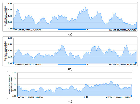
Figure 8.
Spatial distribution of the slump concentration coefficient K values along the Olandų Kepurė cliff: (a) 3 March 2023; (b) 7 April 2023; (c) 24 August 2023.
Our research also indicates a clear seasonal pattern in the occurrence of slumps on various strips of the Olandų Kepurė cliff scarp (Figure 8). Their probability decreases in the spring to early summer period, and a particularly noticeable decrease is in the second part of this period. If the average K value decreased slightly (−0.01) from March to May, from June to August, it decreased significantly (−0.12). This volatility in the seasonal development of cliff scarp slumps is particularly evident in the central, i.e., the highest part of the cliff, where the geomorphology of the cliff is the most complicated [98].
3.3. Spatial Distribution Patterns of the Cliff Base Cavities
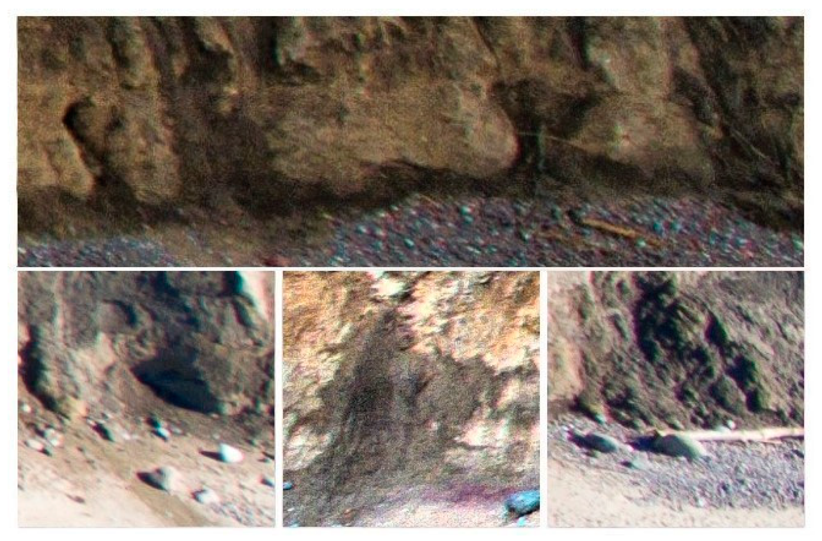
Like in the cases of the cliff scarp slumps, in the case of the Olandų Kepurė cliff, basal cavities would be better labelled as micro-cavities due to their minuscule size (up to 1 m high) and ephemeralness (Figure 9). Yet, one should not underestimate their geomorphological role. Even small cavities forming during the storm surge undercutting the cliff base can induce cliff failure [95,96,97].

Figure 9.
Examples of the Olandų Kepurė cliff base cavities (frontal view taken by a UAV).
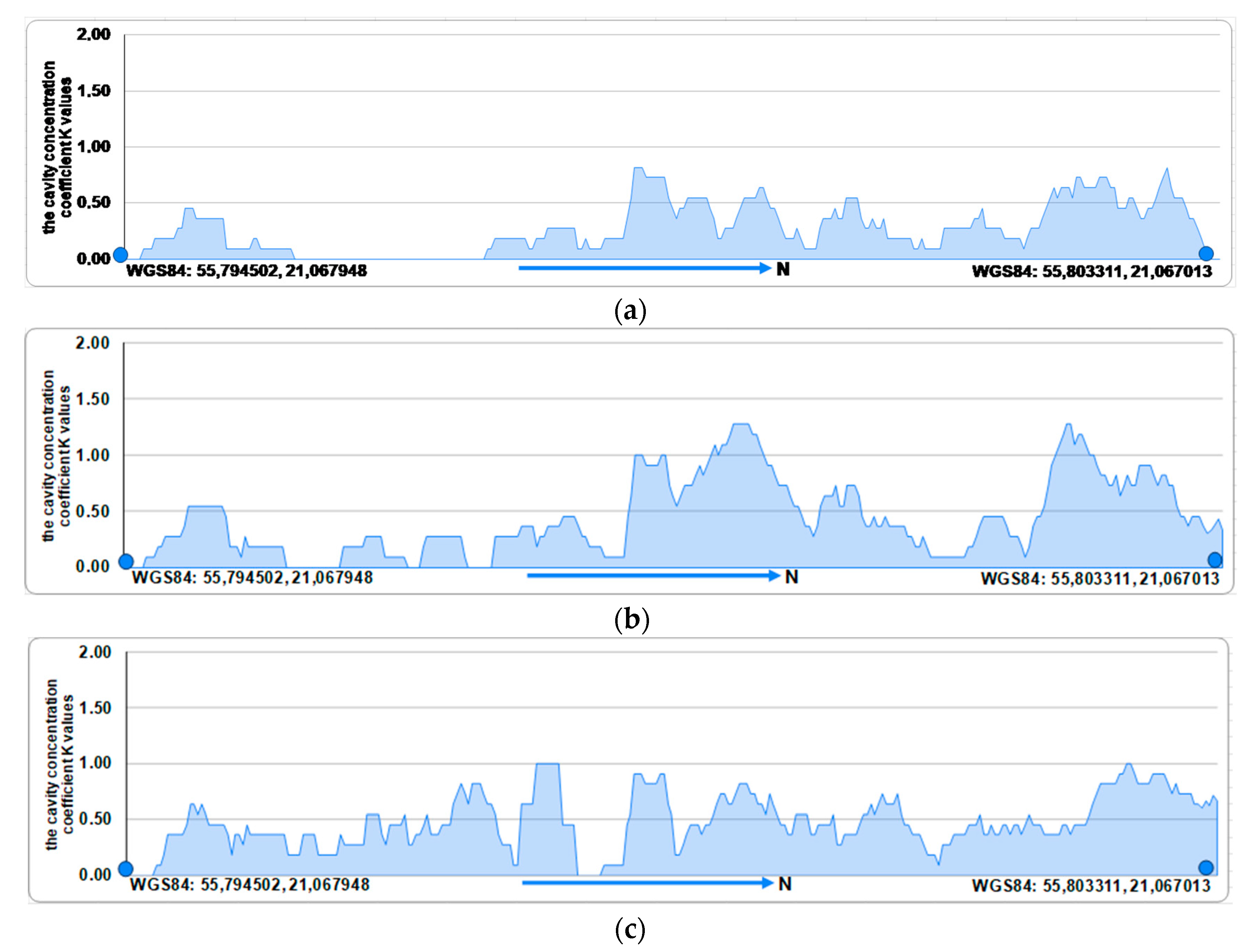
As mentioned, our survey’s most evident quantitative result is that cliff base cavities occur much more seldom than slumps in all three investigated post-storm cases (Figure 10). This feature was especially noticeable in the spring when the occurrence of slumps was 3.5 times more frequent than the occurrence of cliff base cavities. In contrast to slumps, cliff base cavities occurred most frequently in August. The average erosion site concentration coefficient K value, specifically for the concentration of cliff base cavities in all the investigated cells, was 0.26 in March. From April to August, it increased to 0.44.
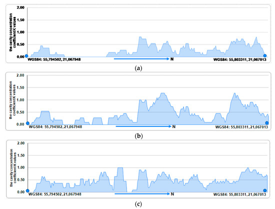
Figure 10.
Spatial distribution of the cavity concentration coefficient K values along the Olandų Kepurė cliff: (a) 3 March 2023; (b) 7 April 2023; (c) 24 August 2023.
Meanwhile, cavities formed by storm waves in the Holocene sand and sandy clay deposits to the south of the cliff’s glacial till strip need to persist longer to be spotted by a UAV. Remarkably, though, even further south, in the southernmost part of the Olandų Kepurė cliff, where sand and sandy clay deposits form the cliff’s base, cavities occurred and were recorded after the storm in August. In this regard, the geomorphological consequences of the late summer storm in terms of the formation of cliff base cavities significantly differ from the consequences of early spring storms.
3.4. Nearshore Hydrodynamics at the Olandų Kepurė Cliff
The volatile calm season development of the Olandų Kepurė cliff scarp slumps and base cavities and the spatiotemporal disentanglement of these two erosion processes feature the complex nature of coastal erosion drivers. The increase in the cliff base cavity development from April to August is most probably related to the slowing down of other erosion processes, which caused relatively more active erosion of the cliff base. However, the Olandų Kepurė cliff is in the temperate Atlantic climate coastal region [99]. Therefore, besides the wave action, other drivers influence the cliff’s geomorphological processes in the calm season, especially in the early spring.
Although wave hydraulic action is often the most pivotal driver of soft cliff erosion, the results of the hydrodynamic modelling of three calm season storm events at the Olandų Kepurė cliff show that during the storms of the calm season, it may not be the case even if the cliff faces westerly or southwesterly wave fetch. Table 1 shows that all three investigated calm season storm events created only a minimal storm surge caused by low wave energy, which dissipated in the foreshore covered in moraine boulders, pebbles, and gravel. Low-energy wave action was due to a seasonal low water level in the Baltic Sea, which is usually in summer.

Table 1.
Modelled parameters of the nearshore hydrodynamics at the Olandų Kepurė cliff.
In the calm season, characterized by the low seasonal water level, a shallow nearshore plays an essential role as a wave energy damping factor. Only the highest, low-probability waves reached the cliff base, creating basal cavities. The nearshore currents had low energy and could not carry away eroded sediments from the foreshore. Such a low-energy wave action explains the disentanglement between the spatial distribution of the observed cliff base cavities and scarp slumps. Therefore, slumps must result from other erosion drivers, most probably seepage caused by rainfall during the storm events.
The results of the hydrodynamic modelling also show that the nearshore currents play an important role during the storms in calm seasons in transporting the eroded sediments from the coast to the nearshore, supplying suspended sand and gravel particles to the resulting northbound longshore littoral sediment drift. It is the pivotal process for ensuring the integrity of the cliff and the adjacent accretion areas as a linear littoral mega-habitat and a littoral cell with erosion and accretion strips [100]. Notably, these litho-dynamic features are coherent with the processes observed in the same South Baltic soft cliffs during autumn and winter stormy periods [101].
The 1455 m long Olandų Kepurė cliff was divided into 5 m long cliff cells, which is sufficient and optimal for determining locations of cliff scarp slumps and base cavities throughout the profile of the cliff. In this way, 291 cliff cells were distinguished. Thus, the cliff erosion clusters, their epicenters and buffers in the horizontal projection of the cliff were determined, distinguishing individual zones of shore activity types.
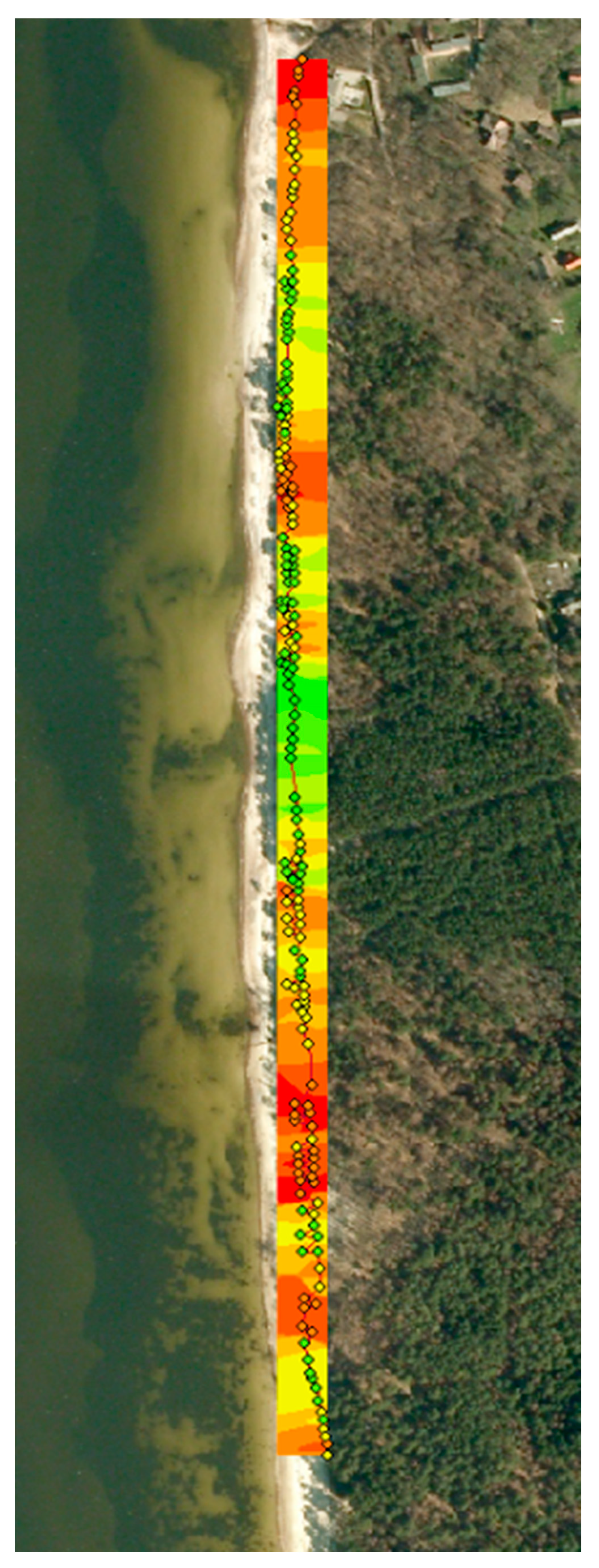
To identify and localize erosion processes and geostatistical analysis of spatial distribution and change, the zones of prevailing shore erosion forms were identified, determining the continuity coefficients K of cells. After transferring the obtained data to a spectrogram, erosion zones were distinguished (Figure 11). It is possible to identify three different behavior zones of the Olandų Kepurė cliff: southern, central, and northern.

Figure 11.
A spectrogram of the prevailing erosion events—slumps in red and cavities in green, the cliff cells where slumps prevail are painted in red, and where cavities prevail are in green.
3.5. Cliff Cells and Behavior Units of the Olandų Kepurė Cliff
Cliff dynamics reflect site conditions; each cliff problem is specific [45]. The interrelated geomorphological processes affect the entire backshore, foreshore, and nearshore [102]. Therefore, it is possible to analyze each cliff-lined coastal area as a strip of a linear littoral habitat representing a narrow block from the cliff top to the nearshore of various lengths featuring similar drivers and geomorphological responses or behaviors. Lee and Clark [45] aptly labelled these strips as cliff behavior units (CBUs). Thus, it is possible to group any cliff of various lengths into CBUs as homogeneous elements [103].
Lee ad Clark argue [45] (p. 10) that “the reason to stress ‘behavior’ is that the interrelationships between both process and form are central to explaining the episodic and uncertain nature of the recession process. In this context it is useful to consider cliffs as open sediment transport systems characterized by inputs, throughputs and outputs of material, i.e., they are cascading systems”.
The CBU concept allows the differentiation of the shoreline management approaches depending on the priorities, e.g., conserving the natural state of an undeveloped protected coast like Olandų Kepurė [102]. Therefore, eliciting CBUs is essential for soft cliff surveillance and management, featuring the long-term links between the cliff’s shape and geomorphological processes. CBUs comprise three coherent sub-systems: cliff top, surface, and foreshore [45]. For a CBU, we need to know the nature of geomorphological events, their magnitude and frequency, and the trends, rates and occurrences of large-scale events shaping the cliff, the foreshore and the nearshore [104].
A CBU as a system comprises two essential components: the shoreline sub-system and the cliff sub-system [105]. The impacts on the CBU include a generalized hierarchy of the environmental activation mechanism and primary responses. A typical feature of many CBUs is the sporadic material supply to the foreshore. For beaches, this will equal an irregular delivery of pebbles, gravel, and sand, resulting in changes in beach volume [45]. Considering more processes (beaches, human action, longshore sediment drift), it is possible to describe the CBU behavior better, and the predictions are closer to reality [103].
The Olando Kepurė cliff is classified as a composite cliff system [45], i.e., in our terminology, a complex linear littoral habitat comprising a partly coupled series of homogeneous CBUs. Based on the results of our investigation, three CBUs were distinguished along the 1.5 km length of the Olando Kepurė cliff, each with specific physical features, sediments, cliff dynamics, and the intensiveness of scarp slump and base cavity formation (Table 2). The output from one CBU may not always necessarily form an input for the next, although the boundaries between them are not strictly demarcated [48].
Table 2.
Cliff behavior units (CBUs) of the Olandų Kepurė cliff.
The southern and central CBUs of the cliff enjoy limited use of the beach, as the narrow foreshore between the cliff and the sea (<50 m) is a bottleneck for visitor flows, especially when the seasonal sea level is high, usually in spring. The cliff is recessing actively in the southern part. The northern CBU is stabilizing and acquiring vegetation and soil cover. In Lee and Clark’s terms, it is a bluff [45], p. 5: “Steep vegetated coastal slopes, termed bluffs, are generally former cliffs degraded by weathering; most are stable”.
4. Discussion
A range of interrelated drivers may cause the detachment of loose material, resulting in soft cliff erosion [95,96]. The most active drivers are:
- Wave action, including hydraulic action and abrasion, and fluid shearing by up-rushing waves during large storms;
- Seepage erosion;
- Surface erosion, i.e., run-off and wind erosion;
- Gravitational mass movement (creep).
In the case of the Olandų Kepurė cliff erosion in the calm season, the most pivotal drivers are wave action, but especially seepage erosion. Lee and Clark [45], p. 33, define seepage erosion as a cliff denudation process involving the detachment and removal of cliff surface particles by the seepage drag of groundwater flowing out of an exposed soil face with the detachment of sand or till particles from degrading landslide blocks and scarp slumps being the primary process. It reduces the resistance of till, resulting in a scarp slump [94]. Water brings eroded particles down the cliff and deposits on the foreshore [45].
Seepage erosion can shape small-scale slumps in loose sediments [104], like in the case of the Olandų Kepurė cliff. However, seepage is an insufficient erosion driver in lithified materials. Hence, seepage erosion is a prevailing erosive process of soft cliffs, which in a moderate climate zone is particularly prominent in spring after the snow melts, the sediment thaws and the saturation of the groundwater layer induces active infiltration into sediments [106,107,108]. Yet, monitoring and measuring seepage erosion processes on soft cliffs using remote sensing methods is more complex than monitoring wave action.
The essential findings of the results of the presented study led to an apparent notion that it was an efficient approach to consider the coasts as 1-D linear objects in the quantitative analysis and monitoring of coastal erosion processes. For instance, it is valuable in modelling the boundaries of littoral (longshore sediment drift) cells as coastal structures [109]. Due to longshore sediment transport, the 1-D coastline model can accommodate essential processes on the coast, such as perpendicular transport to the beach, changes due to sea level rise, and long-term trends in shoreline changes [110].
It is possible to study coastal behavior of a soft cliff as a linear littoral habitat if sufficient precision of remote sensing using UAVs is achieved and a linear (1-D) interpretation using ArcGIS is applied. Erosion processes of coastal cliffs, especially those with slow retreat rates, are notoriously difficult to monitor by remote sensing methods [111,112,113]. Hence, the advantage of interpreting the eroded coast as a 1-D linear littoral habitat surveyed and monitored by applying the combined approach of the UAV-based field surveillance with data storage and analysis in the ArcGIS-based 1-D database.
The novelty of the results lies in a comprehensive conceptual interpretation and analysis of the eroded coast as a linear littoral habitat. Despite its narrowness, or maybe because of it, this complex linear littoral habitat is a dynamic boundary between the aquatic areal habitats and the terrestrial ones. It is, by convention, the structural element which, in remote sensing interpretation, is referred to as the “instantaneous shoreline” [114].
From the perspective of previous studies, the central practical aspect of the presented study as an illustration of the littoral habitat concept is the deliberation of coastal squeeze as a coastal conservation and management challenge. The development of coastal green infrastructure as a cliff management strategy may deal with a coastal squeeze in eight steps [115]: adequate diagnosis; conservation of mass and energy fluxes; mimicry of natural functions; use of local resources; local actor participation; design and adaptation of solution; resistance and resilience of the intervention; adaptability of the solution. Monitoring is essential in all eight steps.
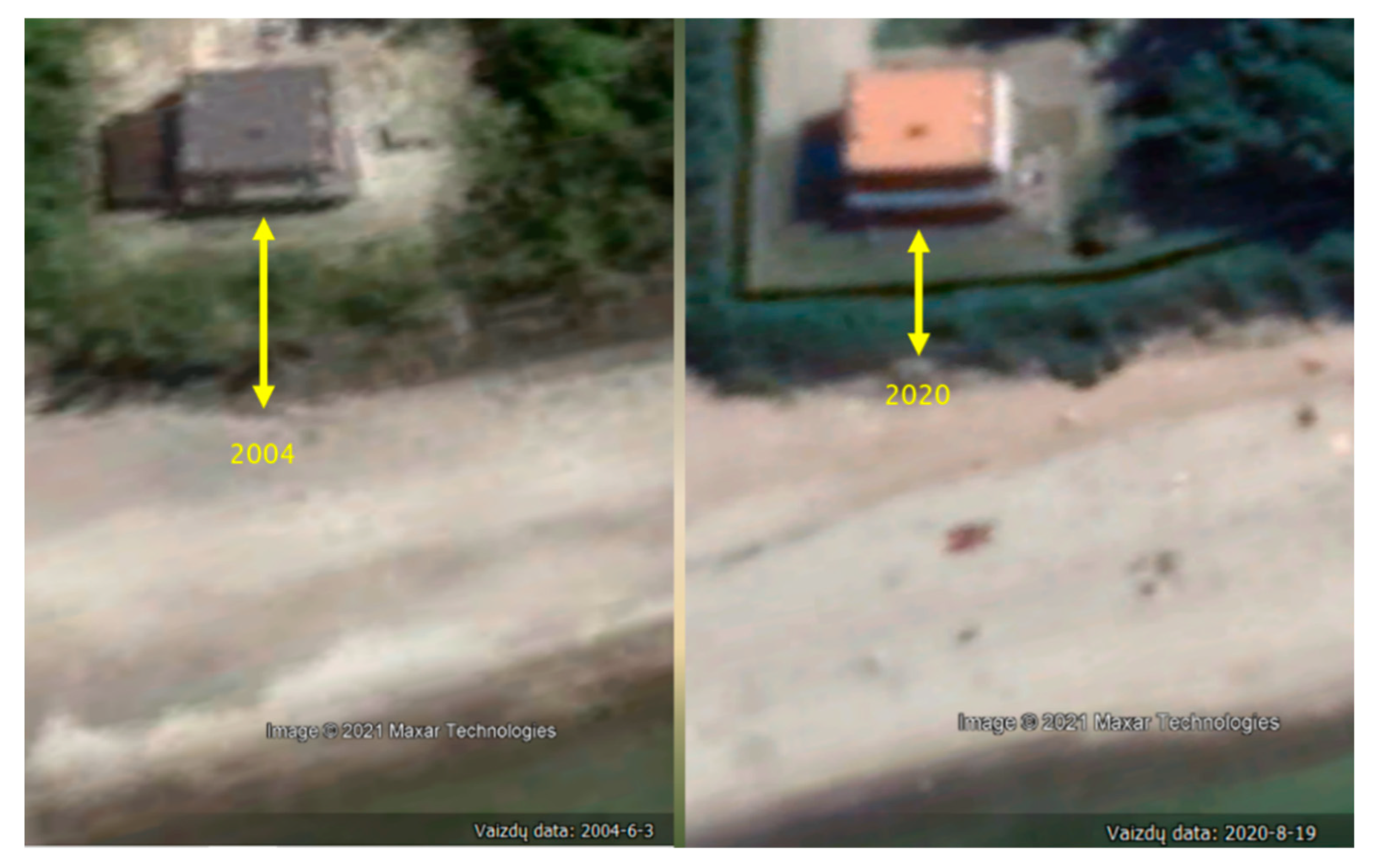
Also, active communication among scientists, decision-makers and local stakeholders is necessary. Despite Olandų Kepurė being a managed nature reserve, there is one site on the northern part of the cliff top threatened by a coastal squeeze where relocation is impossible as a management strategy (Figure 12). The project developers should involve local stakeholders. They should contribute to the design, implementation, and monitoring processes. In this way, the scientific community will propagate the coastal squeeze mitigation strategies to balance natural processes with human interests and needs [12,116].

Figure 12.
An example of ‘coastal squeeze’ at the Olandų Kepurė cliff (Satellite image credit: © GoogleEarthTM, Mountain View, CA, USA).
Coastal cliff management needs an awareness of geomorphology and changes resulting from coastal processes [117]. It typically aims to break the cliff recession or reduce it. However, what if the cliff is in a managed nature reserve protected as a natural monument? In the UK, cliffs are the most significant landscape assets protected within National Parks and Areas of Outstanding Natural Beauty or as heritage coasts [45]. Cliffs are biodiversity reservoirs with many plant species and communities of coastal cliffs protected by Council Directive 92/43/EEC, and their monitoring is obligatory in EU countries [118].
The essential limitation of the work is the accuracy of the UAV measurements of the cliff surface at a non-vertical angle. Another limitation of the study is in possible human error in the identification process of the erosion sites—cliff scarp slumps and cliff base cavities. We made efforts to eliminate any human error, which the Delphi method enables in such studies. In our opinion, the varying spatial distribution of erosion sites during the investigated storms, which occurred in calm periods, has natural causes and it is not caused by a human error.
It should be an important, albeit not pivotal, method in a broader, comprehensive littoral monitoring system combining methods to survey coastal slope, orientation, geology, substrate, wave exposure, water temperature, human impact, and their impact on the distribution of littoral habitats [119]. Combining the usage of UAV with GIS analysis tools enables researchers to recognize and map the cliff plant species, derive and measure the habitat and species distribution area, count surveyed individuals, and gather quantitative data on their projected area [118].
Future research directions in combining the application of UAVs with GIS tools for coastal cliff surveys will focus on technological improvements in UAVs to help tackle the image quality problem. AI algorithms will become more efficient in recognizing cliff scarp slumps, foot cavities and other ephemeral forms resulting from coastal erosion processes. Machine learning techniques are popular for classifying regularly acquired remotely sensed imagery [120]. The latest promising techniques include regression-based applications of deep learning models for multi-scale image detection on UAVs, which are more effective than the models with a small number of trainable parameters [121].
5. Conclusions
We tested using a UAV as a survey means, gathering remote sensing images of the Olandų Kepurė cliff (eastern Baltic Sea coast, Lithuania). Five photo interpreters independently analyzed the acquired images using the Delphi technique. Using ArcGIS, the distribution of cliff scarp slumps and cliff base cavities as the main ephemeral geomorphological features resulting from coastal erosion processes was mapped. The main conclusion is that the survey results were not affected by photo interpreters and are of sufficient discerning quality for decision making in cliff conservation and management.
By increasing the density of surveyed cliff cells in the analysis of the distribution of slumps and cavities, the results become more uniform, and by reducing the density of surveyed cliff cells, the results become more fragmented. After performing initial calculations using cliff cells of different lengths, the conclusion is that a 55 m long cliff cell is the most suitable to analyze cliff behavior. This insight led to the further conclusion that there is no direct relationship between wave action and the cavity and slump formation. The behavior of the Olandų Kepurė cliff is complex and, during the calm season, depends primarily on seepage erosion.
Even though the Olandų Kepurė cliff is a unique coastal strip for the Lithuanian Baltic Sea coast, it is not included in the National Coastal Belt Management Program for 2023–2032 approved by the Lithuanian Government. Therefore, no specific coastal management measures are designed for the cliff. Since it is Lithuania’s most visited natural object, such a situation is paradoxical. Nevertheless, various soft cliff management measures related to visitor flow management are implemented yearly, such as installing wooden paths and stairs down to the beach. The key challenge is understanding the cliff behavior in different seasons and weather conditions.
Author Contributions
Conceptualization, E.J., A.U. and R.P.; methodology, E.J. and J.T.; software, E.J., J.M. and D.U.; validation, R.P. and J.T.; formal analysis, E.J.; investigation, E.J., R.P. and A.U.; resources, R.P.; data curation, E.J.; writing—original draft preparation, E.J.; writing—review and editing, R.P.; visualization, E.J.; supervision, R.P.; project administration, E.J.; funding acquisition, E.J. All authors have read and agreed to the published version of the manuscript.
Funding
This research was funded by the Administration of Lithuania Minor Protected Areas from its statutory coastal monitoring budget.
Institutional Review Board Statement
Not applicable.
Informed Consent Statement
Not applicable.
Data Availability Statement
The data presented in this study are available on request from the corresponding author.
Acknowledgments
The authors would like to thank Simonas Bendikas and other personnel of the Administration of Lithuania Minor Protected Areas for their help during the data collection.
Conflicts of Interest
The authors declare no conflicts of interest. The funders had no role in the design of the study; in the collection, analyses, or interpretation of data; in the writing of the manuscript; nor in the decision to publish the results.
References
- Robles-Diaz-de-León, L.F.; Nava-Tudela, A. Playing with Asimina triloba (pawpaw): A species to consider when enhancing riparian forest buffer systems with non-timber products. Ecol. Model. 1998, 112, 169–193. [Google Scholar] [CrossRef]
- Povilanskas, R.; Armaitienė, A.; Breber, P.; Razinkovas-Baziukas, A.; Taminskas, J. The Integrity of Linear Littoral Habitats of Lesina and Curonian Lagoons. Hydrobiologia 2012, 699, 99–110. [Google Scholar] [CrossRef]
- Povilanskas, R.; Chubarenko, B.V. Interaction between the drifting dunes of the Curonian Barrier Spit and the Curonian Lagoon. Baltica 2000, 13, 8–14. [Google Scholar]
- Povilanskas, R.; Riepšas, E.; Armaitienė, A.; Dučinskas, K.; Taminskas, J. Shifting Dune Types of the Curonian Spit and Factors of Their Development. Balt. For. 2011, 17, 215–226. [Google Scholar]
- Povilanskas, R. Landscape Management on the Curonian Spit: A Cross-Border Perspective; EUCC Publishers: Klaipeda, Lithuania, 2004; 242p. [Google Scholar]
- Šimanauskienė, R.; Linkevičienė, R.; Povilanskas, R.; Satkūnas, J.; Veteikis, D.; Baubinienė, A.; Taminskas, J. Curonian Spit coastal dunes landscape: Climate driven change calls for the management optimization. Land 2022, 11, 877. [Google Scholar] [CrossRef]
- Zhu, E.; Gao, H.; Chen, L.; Yao, J.; Liu, T.; Sha, M. Interactions between coastal protection forest ecosystems and human activities: Quality, service and resilience. Ocean Coast. Manag. 2024, 254, 107190. [Google Scholar] [CrossRef]
- Danial, H.; Syahrul, S.S.; Muhammad, Y. A Model of Fish Marketing at Paotere Fishing Ports for Increasing Fishermen’s Income. Int. J. Dev. Res. 2018, 8, 20013–20018. [Google Scholar]
- Doody, J.P. Sand Dune Conservation, Management and Restoration; Springer: Dordrecht, The Netherlands, 2013; 304p. [Google Scholar]
- Pontee, N. Defining coastal squeeze: A discussion. Ocean Coast. Manag. 2013, 84, 204–207. [Google Scholar] [CrossRef]
- Doody, J.P. ‘Coastal squeeze’—An historical perspective. J. Coast. Conserv. 2004, 10, 129–138. [Google Scholar] [CrossRef]
- Silva, R.; Martínez, M.L.; van Tussenbroek, B.I.; Guzmán-Rodríguez, L.O.; Mendoza, E.; López-Portillo, J. A framework to manage coastal squeeze. Sustainability 2020, 12, 10610. [Google Scholar] [CrossRef]
- Jordan, P.; Fröhle, P. Bridging the gap between coastal engineering and nature conservation? A review of coastal ecosystems as nature-based solutions for coastal protection. J. Coast. Conserv. 2022, 26, 4. [Google Scholar] [CrossRef]
- Pörtner, H.O.; Roberts, D.C.; Masson-Delmotte, V. The Ocean and Cryosphere in a Changing Climate: Special Report of the Intergovernmental Panel on Climate Change; Cambridge University Press: Cambridge, UK, 2022; 756p. [Google Scholar]
- Luijendijk, A.; Hagenaars, G.; Ranasinghe, R.; Baart, F.; Donchyts, G.; Aarninkhof, S. The state of the world’s beaches. Sci. Rep. 2018, 8, 6641. [Google Scholar] [CrossRef] [PubMed]
- Er-Ramy, N.; Nachite, D.; Anfuso, G.; Williams, A.T. Coastal scenic quality assessment of Moroccan Mediterranean beaches: A tool for proper management. Water 2022, 14, 1837. [Google Scholar] [CrossRef]
- Yasmeen, A.; Pumijumnong, N.; Arungrat, N.; Punwong, P.; Sereenonchai, S.; Chareonwong, U. Nature-based solutions for coastal erosion protection in a changing climate: A cutting-edge analysis of contexts and prospects of the muddy coasts. Estuar. Coast. Shelf Sci. 2024, 298, 108632. [Google Scholar] [CrossRef]
- Jurkus, E.; Povilanskas, R.; Taminskas, J. Current Trends and Issues in Research on Biodiversity Conservation and Tourism Sustainability. Sustainability 2022, 14, 3342. [Google Scholar] [CrossRef]
- Jurkus, E.; Povilanskas, R.; Razinkovas-Baziukas, A.; Taminskas, J. Current trends and issues in applications of remote sensing for coastal and marine nature conservation. Earth 2022, 3, 433–447. [Google Scholar] [CrossRef]
- Chen, H. The ecosystem service value of maintaining and expanding terrestrial protected areas in China. Sci. Total Environ. 2021, 781, 146768. [Google Scholar] [CrossRef] [PubMed]
- Fennell, D.A. Ecotourism, 5th ed.; Routledge: Oxon, UK; New York, NY, USA, 2020; xviii + 282p. [Google Scholar]
- Schirpke, U.; Meisch, C.; Tappeiner, U. Symbolic species as a cultural ecosystem service in the European Alps: Insights and open issues. Landsc. Ecol. 2018, 33, 711–730. [Google Scholar] [CrossRef]
- Chun, J.; Kim, C.K.; Kim, G.S.; Jeong, J.; Lee, W.K. Social big data informs spatially explicit management options for national parks with high tourism pressures. Tour. Manag. 2020, 81, 104136. [Google Scholar] [CrossRef]
- Dalton, D.T.; Pascher, K.; Berger, V.; Steinbauer, K.; Jungmeier, M. Novel Technologies and Their Application for Protected Area Management: A Supporting Approach in Biodiversity Monitoring. In Protected Area Management-Recent Advances; Nazip Suratman, M., Ed.; IntechOpen: London, UK, 2021; Available online: https://www.intechopen.com/chapters/78656 (accessed on 1 February 2022).
- Smith, M.K.S.; Smit, I.P.; Swemmer, L.K.; Mokhatla, M.M.; Freitag, S.; Roux, D.J.; Dziba, L. Sustainability of protected areas: Vulnerabilities and opportunities as revealed by COVID-19 in a national park management agency. Biol. Conserv. 2021, 255, 108985. [Google Scholar] [CrossRef]
- Cheung, S.Y.; Leung, Y.F.; Larson, L.R. Citizen science as a tool for enhancing recreation research in protected areas: Applications and opportunities. J. Environ. Manag. 2022, 305, 114353. [Google Scholar] [CrossRef] [PubMed]
- Ferreira, C.C.; Stephenson, P.J.; Gill, M.; Regan, E.C. Biodiversity Monitoring and the Role of Scientists in the Twenty-first Century. In Closing the Knowledge-Implementation Gap in Conservation Science; Ferreira, C.C., Klütsch, C.F.C., Eds.; Springer: Cham, Switzerland, 2021; pp. 25–50. [Google Scholar]
- Suškevičs, M.; Raadom, T.; Vanem, B.; Kana, S.; Roasto, R.; Runnel, V.; Külvik, M. Challenges and opportunities of engaging biodiversity-related citizen science data in environmental decision-making: Practitioners’ perceptions and a database analysis from Estonia. J. Nat. Conserv. 2021, 64, 126068. [Google Scholar] [CrossRef]
- Heberling, J.M.; Miller, J.T.; Noesgaard, D.; Weingart, S.B.; Schigel, D. Data integration enables global biodiversity synthesis. Proc. Natl. Acad. Sci. USA 2021, 118, e2018093118. [Google Scholar] [CrossRef]
- Jessen, T.D.; Ban, N.C.; Claxton, N.X.; Darimont, C.T. Contributions of Indigenous Knowledge to ecological and evolutionary understanding. Front. Ecol. Environ. 2022, 20, 93–101. [Google Scholar] [CrossRef]
- Mi, X.; Feng, G.; Hu, Y.; Zhang, J.; Chen, L.; Corlett, R.T.; Hughes, A.C.; Pimm, S.; Schmid, B.; Shi, S.; et al. The global significance of biodiversity science in China: An overview. Nat. Sci. Rev. 2021, 8, nwab032. [Google Scholar] [CrossRef] [PubMed]
- Gardel, A.; Anthony, E.J.; Santos, V.F.; Huybrechts, N.; Lesourd, S.; Sottolichio, A.; Maury, T. A remote sensing-based classification approach for river mouths of the Amazon-influenced Guianas coast. Region. Environ. Change 2022, 22, 65. [Google Scholar] [CrossRef]
- Moniruzzaman, M.; Islam, S.M.; Lavery, P.; Bennamoun, M.; Lam, C.P. Imaging and classification techniques for seagrass mapping and monitoring: A comprehensive survey. arXiv 2019, arXiv:1902.11114. [Google Scholar]
- Orusa, T.; Borgogno Mondino, E. Exploring Short-term climate change effects on rangelands and broad-leaved forests by free satellite data in Aosta Valley (Northwest Italy). Climate 2021, 9, 47. [Google Scholar] [CrossRef]
- da Silveira, C.B.L.; Strenzel, G.M.R.; Maida, M.; Gaspar, A.L.B.; Ferreira, B.P. Coral Reef Mapping with Remote Sensing and Machine Learning: A Nurture and Nature Analysis in Marine Protected Areas. Remote Sens. 2021, 13, 2907. [Google Scholar] [CrossRef]
- Failler, P.; Touron-Gardic, G.; Sadio, O.; Traoré, M.S. Perception of natural habitat changes of West African marine protected areas. Ocean Coast. Manag. 2020, 187, 105120. [Google Scholar] [CrossRef]
- Singh, A.A.; Maharaj, A.; Singh, P. Benthic Resource Baseline Mapping of Cakaunisasi and Yarawa Reef Ecosystem in the Ba Region of Fiji. Water 2021, 13, 468. [Google Scholar] [CrossRef]
- Costello, M.J.; Darnaedi, D.; Diway, B.; Ganyai, T.; Grudpan, C.; Hughes, A.; Ishii, R.; Lim, P.T.; Ma, K.; Muslim, A.M.; et al. The Asia-Pacific Biodiversity Observation Network: 10-year achievements and new strategies to 2030. Ecol. Res. 2021, 36, 232–257. [Google Scholar]
- Visalli, M.E.; Best, B.D.; Cabral, R.B.; Cheung, W.W.L.; Clark, N.A.; Garilao, C.; Kaschner, K.; Kesner-Reyes, K.; Lam, V.W.Y.; Maxwell, S.M.; et al. Data-driven approach for highlighting priority areas for protection in marine areas beyond national jurisdiction. Mar. Policy 2020, 122, 103927. [Google Scholar] [CrossRef]
- Wang, Y.; Lu, Z.; Sheng, Y.; Zhou, Y. Remote sensing applications in monitoring of protected areas. Remote Sens. 2020, 12, 1370. [Google Scholar] [CrossRef]
- El Mahrad, B.; Newton, A.; Icely, J.D.; Kacimi, I.; Abalansa, S.; Snoussi, M. Contribution of remote sensing technologies to a holistic coastal and marine environmental management framework: A review. Remote Sens. 2020, 12, 2313. [Google Scholar] [CrossRef]
- Kachelreiss, D.; Wegmann, M.; Gollock, M.; Pettorelli, N. The application of remote sensing for marine protected area management. Ecol. Indic. 2014, 36, 169–177. [Google Scholar] [CrossRef]
- Topouzelis, K.; Papakonstantinou, A.; Singha, S.; Li, X.; Poursanidis, D. Editorial on Special Issue “Applications of Remote Sensing in Coastal Areas”. Remote Sens. 2020, 12, 974. [Google Scholar] [CrossRef]
- Adade, R.; Aibinu, A.M.; Ekumah, B.; Asaana, J. Unmanned Aerial Vehicle (UAV) applications in coastal zone management—A review. Environ. Monit. Assess. 2021, 193, 154. [Google Scholar] [CrossRef] [PubMed]
- Lee, E.M.; Clark, A.R. Investigation and Management of Soft Rock Cliffs; Telford Publishing: London, UK, 2002; 382p. [Google Scholar]
- Gelumbauskaitė, L.Ž. On the morphogenesis and morphodynamics of the shallow zone off the Kuršių Nerija (Curonian Spit). Baltica 2003, 16, 37–42. [Google Scholar]
- Komar, P.D. Computer models of shoreline configuration: Headland erosion and the graded beach revisited. In Models in Geomorphology, 2nd ed.; Woldenberg, M.J., Ed.; Routledge: Abington, UK; New York, NY, USA, 2020; pp. 155–170. [Google Scholar]
- Povilanskas, R.; Urbis, A. National ICZM strategy and initiatives in Lithuania. Coastline Rep. 2004, 2, 9–15. [Google Scholar]
- Masoodian, S.A. Sistan’s 120 Days Wind. J. Appl. Climatol. 2014, 1, 37–46. [Google Scholar]
- Dailidė, R.; Dailidė, G.; Razbadauskaitė-Venskė, I.; Povilanskas, R.; Dailidienė, I. Sea-breeze front research based on remote sensing methods in coastal Baltic Sea climate: Case of Lithuania. J. Mar. Sci. Eng. 2022, 10, 1779. [Google Scholar] [CrossRef]
- Soomere, T.; Weisse, R.; Behrens, A. Wave climatology in the Arkona Basin, the Baltic Sea. Ocean Sci. Discuss. 2011, 8, 2237–2270. [Google Scholar]
- Dacre, H.F.; Gray, S.L. The spatial distribution and evolution characteristics of North Atlantic cyclones. Mon. Weather Rev. 2009, 137, 99–115. [Google Scholar] [CrossRef]
- Climate. Ranger’s Office of Littoral Regional Park. Available online: https://www.pajuris.info/ (accessed on 19 December 2024). (In Lithuanian).
- Baltranaitė, E.; Jurkus, E.; Povilanskas, R. Impact of Physical Geographical Factors on Sustainable Planning of South Baltic Seaside Resorts. Baltica 2017, 30, 119–131. [Google Scholar] [CrossRef]
- Jurkus, E.; Taminskas, J.; Povilanskas, R.; Kontautienė, V.; Baltranaitė, E.; Dailidė, R.; Urbis, A. Delivering tourism sustainability and competitiveness in seaside and marine resorts with GIS. J. Mar. Sci. Eng. 2021, 9, 312. [Google Scholar] [CrossRef]
- Povilanskas, R.; Armaitienė, A.; Jones, E.; Valtas, G.; Jurkus, E. Third-Country Tourists on the Ferries linking Germany with Lithuania. Scand. J. Hosp. Tour. 2015, 15, 327–340. [Google Scholar] [CrossRef]
- Povilanskas, R.; Razinkovas-Baziukas, A.; Jurkus, E. Integrated environmental management of transboundary transitional waters: Curonian Lagoon case study; Ocean Coast. Manag. 2014, 101, 14–23. [Google Scholar] [CrossRef]
- Urbis, A.; Povilanskas, R.; Jurkus, E.; Taminskas, J.; Urbis, D. GIS-based aesthetic appraisal of short-range viewsheds of coastal dune and forest landscapes. Forests 2021, 12, 1534. [Google Scholar] [CrossRef]
- Povilanskas, R.; Satkūnas, J.; Jurkus, E. Conditions for deep geothermal energy utilisation in southwest Latvia: Nīca case study. Baltica 2013, 26, 193–200. [Google Scholar] [CrossRef]
- Urbis, A.; Povilanskas, R.; Šimanauskienė, R.; Taminskas, J. Key aesthetic appeal concepts of coastal dunes and forests on the example of the Curonian Spit (Lithuania). Water 2019, 11, 1193. [Google Scholar] [CrossRef]
- Barzehkar, M.; Parnell, K.E.; Soomere, T.; Dragovich, D.; Engström, J. Decision support tools, systems and indices for sustainable coastal planning and management: A review. Ocean Coast. Manag. 2021, 212, 105813. [Google Scholar] [CrossRef]
- Kostopoulou, E. Applicability of ordinary Kriging modeling techniques for filling satellite data gaps in support of coastal management. Model. Earth Syst. Environ. 2021, 7, 1145–1158. [Google Scholar] [CrossRef]
- Parthasarathy, K.S.S.; Deka, P.C. Remote sensing and GIS application in assessment of coastal vulnerability and shoreline changes: A review. ISH J. Hydraul. Eng. 2021, 27 (Suppl. S1), 588–600. [Google Scholar] [CrossRef]
- Yasir, M.; Hui, S.; Binghu, H.; Rahman, S.U. Coastline extraction and land use change analysis using remote sensing (RS) and geographic information system (GIS) technology–A review of the literature. Rev. Environ. Health 2020, 35, 453–460. [Google Scholar] [CrossRef] [PubMed]
- Taylor, E. We agree, don’t we? The Delphi method for health environments research. HERD Health Environ. Res. Des. J. 2020, 13, 11–23. [Google Scholar] [CrossRef] [PubMed]
- Boulkedid, R.; Abdoul, H.; Loustau, M.; Sibony, O.; Alberti, C. Using and reporting the Delphi method for selecting healthcare quality indicators: A systematic review. PLoS ONE 2011, 6, e20476. [Google Scholar] [CrossRef] [PubMed]
- Garrod, B.; Fyall, A. Managing Heritage Tourism. Ann. Tour. Res. 2000, 27, 682–708. [Google Scholar] [CrossRef]
- Hsu, C.C.; Sandford, B.A. The Delphi technique: Making sense of consensus. Pract. Assess. Res. Eval. 2007, 12, 10. [Google Scholar]
- Gobster, P.H.; Schneider, I.E.; Floress, K.M.; Haines, A.L.; Arnberger, A.; Dockry, M.J.; Benton, C. Understanding the key characteristics and challenges of pine barrens restoration: Insights from a Delphi survey of forest land managers and researchers. Restor. Ecol. 2021, 29, 13273. [Google Scholar] [CrossRef]
- La Sala, P.; Conto, F.; Conte, A.; Fiore, M. Cultural Heritage in Mediterranean Countries: The Case of an IPA Adriatic Cross Border Cooperation Project. Int. J. Eur. Med. Stud. 2016, 9, 31–50. [Google Scholar]
- Lupp, G.; Konold, W.; Bastian, O. Landscape management and landscape changes towards more naturalness and wilderness: Effects on scenic qualities—The case of the Muritz National Park in Germany. J. Nat. Conserv. 2013, 21, 10–21. [Google Scholar] [CrossRef]
- Monavari, S.M.; Khorasani, N.; Mirsaeed, S.S.G. Delphi-based Strategic Planning for Tourism Management–A Case Study. Pol. J. Environ. Stud. 2013, 22, 465–473. [Google Scholar]
- Olszewska, A.A.; Marques, P.F.; Ryan, R.L.; Barbosa, F. What makes a landscape contemplative? Environ. Plann. B 2018, 45, 7–25. [Google Scholar] [CrossRef]
- Tan, W.J.; Yang, C.F.; Château, P.A.; Lee, M.T.; Chang, Y.C. Integrated coastal-zone management for sustainable tourism using a decision support system based on system dynamics: A case study of Cijin, Kaohsiung, Taiwan. Ocean Coast. Manag. 2018, 153, 131–139. [Google Scholar] [CrossRef]
- Umgiesser, G.; Melaku Canu, D.; Cucco, A.; Solidoro, C. A finite element model for the Venice Lagoon, Development, set up, calibration and validation. J. Mar. Syst. 2004, 51, 123–145. [Google Scholar] [CrossRef]
- Umgiesser, G. Modelling the Venice Lagoon. Int. J. Salt Lake Res. 1997, 6, 175–199. [Google Scholar] [CrossRef]
- Ferrarin, C.; Umgiesser, G. Hydrodynamic modeling of a coastal lagoon: The Cabras lagoon in Sardinia, Italy. Ecol. Model. 2005, 188, 340–357. [Google Scholar] [CrossRef]
- Ferrarin, C.; Umgiesser, G.; Bajo, M.; Bellafiore, D.; De Pascalis, F.; Ghezzo, M.; Mattassi, G.; Scroccaro, I. Hydraulic zonation of the lagoons of Marano and Grado, Italy. A modelling approach. Estuar. Coast. Shelf Sci. 2010, 87, 561–572. [Google Scholar] [CrossRef]
- Bellafiore, D.; Umgiesser, G. Hydrodynamic coastal processes in the North Adriatic investigated with a 3-D finite element model. Ocean Dyn. 2010, 60, 255–276. [Google Scholar] [CrossRef]
- Bellafiore, D.; Guarnieri, A.; Grilli, F.; Penna, P.; Bortoluzzi, G.; Giglio, F.; Pinardi, N. Study of the hydrodynamical processes in the Boka Kotorska Bay with a finite element model. Dyn. Atmos. Ocean. 2011, 52, 298–321. [Google Scholar] [CrossRef]
- De Pascalis, F.; Pérez-Ruzafa, A.; Gilabert, J.; Marcos, C.; Umgiesser, G. Climate change response of the Mar Menor coastal lagoon (Spain) using a hydrodynamic finite element model. Estuar. Coast. Shelf Sci. 2011, 114, 118–129. [Google Scholar] [CrossRef]
- Zemlys, P.; Ferrarin, C.; Umgiesser, G.; Gulbinskas, S.; Bellafiore, D. Investigation of saline water intrusions into the Curonian Lagoon (Lithuania) and two-layer flow in the Klaipėda Strait using finite element hydrodynamic model. Ocean Sci. 2013, 9, 573–584. [Google Scholar] [CrossRef]
- Umgiesser, G.; Ferrarin, C.; Cucco, A.; De Pascalis, F.; Bellafiore, D.; Ghezzo, M.; Bajo, M. Comparative hydrodynamics of 10 Mediterranean lagoons by means of numerical modeling. J. Geophys. Res. 2014, 119, 2212–2226. [Google Scholar] [CrossRef]
- Arpaia, L.; Ferrarin, C.; Bajo, M.; Umgiesser, G. A flexible z-layers approach for the accurate representation of free surface flows in a coastal ocean model (SHYFEM v. 7_5_71). Geosci. Model Dev. 2023, 16, 6899–6919. [Google Scholar] [CrossRef]
- Čerkasova, N.; Mėžinė, J.; Idzelytė, R.; Lesutienė, J.; Ertürk, A.; Umgiesser, G. Exploring variability in climate change projections on the Nemunas River and Curonian Lagoon: Coupled SWAT and SHYFEM modeling approach. Ocean Sci. 2024, 20, 1123–1147. [Google Scholar] [CrossRef]
- Apostolopoulos, D.; Nikolakopoulos, K. A review and meta-analysis of remote sensing data, GIS methods, materials and indices used for monitoring the coastline evolution over the last twenty years. Eur. J. Remote Sens. 2021, 54, 240–265. [Google Scholar] [CrossRef]
- Alberico, I.; Casalbore, D.; Pelosi, N.; Tonielli, R.; Calidonna, C.; Dominici, R.; De Rosa, R. Remote Sensing and Field Survey Data Integration to Investigate on the Evolution of the Coastal Area: The Case Study of Bagnara Calabra (Southern Italy). Remote Sens. 2022, 14, 2459. [Google Scholar] [CrossRef]
- Abualtayef, M.; Rabou, M.A.; Afifi, S.; Rabou, A.F.A.; Seif, A.K.; Masria, A. Change detection of Gaza coastal zone using GIS and remote sensing techniques. J. Coast. Conserv. 2021, 25, 36. [Google Scholar] [CrossRef]
- Sun, W.; Chen, C.; Liu, W.; Yang, G.; Meng, X.; Wang, L.; Ren, K. Coastline extraction using remote sensing: A review. GIS Sci. Remote Sens. 2023, 60, 2243671. [Google Scholar] [CrossRef]
- Zhou, X.; Wang, J.; Zheng, F.; Wang, H.; Yang, H. An Overview of Coastline Extraction from Remote Sensing Data. Remote Sens. 2023, 15, 4865. [Google Scholar] [CrossRef]
- Makar, A. Limitations of multi-GNSS positioning of USV in area with high harbour infrastructure. Electronics 2023, 12, 697. [Google Scholar] [CrossRef]
- Veličković, N.; Todosijević, M.; Šulić, D. Erosion Map Reliability Using a Geographic Information System (GIS) and Erosion Potential Method (EPM): A Comparison of Mapping Methods, BELGRADE Peri-Urban Area, Serbia. Land 2022, 11, 1096. [Google Scholar] [CrossRef]
- Yan, H. Quantifying spatial similarity for use as constraints in map generalisation. J. Spatial Sci. 2024, 69, 23–42. [Google Scholar] [CrossRef]
- Tarbuck, E.J.; Lutgens, F.K.; Tasa, D.G. Earth Science, Global Edition; Pearson Education Limited: Harlow, UK, 2015; 802p. [Google Scholar]
- Sunamura, T. Geomorphology of Rocky Coasts; Wiley: Chichester, UK, 1992; 302p. [Google Scholar]
- Sunamura, T. Rocky coast processes: With special reference to the recession of soft rock cliffs. Proc. Jpn. Acad. Ser. B 2015, 91, 481–500. [Google Scholar] [CrossRef] [PubMed]
- Wolters, G.; Müller, G. Effect of cliff shape on internal stresses and rock slope stability. J. Coast. Res. 2008, 24, 43–50. [Google Scholar] [CrossRef]
- Bitinas, A. Quaternary deposits on the outcrop Olandų Kepurė. In Proceedings of the 5th International Conference of Marine Geology. Abstracts & Excursion Guide, Vilnius, Lithuania, 6–10 October 1997; Grigelis, A., Ed.; Institute of Geology: Vilnius, Lithuania, 1997; pp. 109–110. [Google Scholar]
- Povilanskas, R.; Jurkienė, A.; Dailidienė, I.; Ernšteins, R.; Newton, A.; Leyva Ollivier, M.E. Circles of Coastal Sustainability and Emerald Growth Perspectives for Transitional Waters Under Human Stress. Sustainability 2024, 16, 2544. [Google Scholar] [CrossRef]
- Bertoni, D.; Bini, M.; Luppichini, M.; Cipriani, L.E.; Carli, A.; Sarti, G. Anthropogenic impact on beach heterogeneity within a littoral cell (northern Tuscany, Italy). J. Mar. Sci. Eng. 2021, 9, 151. [Google Scholar] [CrossRef]
- Terefenko, P.; Giza, A.; Śledziowski, J.; Paprotny, D.; Bučas, M.; Kelpšaitė-Rimkienė, L. Classification of soft cliff dynamics using remote sensing and data mining techniques. Sci. Total Environ. 2024, 947, 174743. [Google Scholar] [CrossRef] [PubMed]
- Brunsden, D.; Moore, R. Engineering geomorphology on the coast: Lessons from west Dorset. Geomorphology 1999, 31, 391–409. [Google Scholar] [CrossRef]
- Castedo, R.; Murphy, W.; Lawrence, J.; Paredes, C. A new process–response coastal recession model of soft rock cliffs. Geomorphology 2012, 177, 128–143. [Google Scholar] [CrossRef]
- Higgins, C.G.; Osterkamp, W.R. (Eds.) Seepage-Induced Cliff Recession and Regional Denudation. Groundwater Geomorphology–The Role of Subsurface Water in Earth Surface Processes and Landforms. Special Paper 252; Geological Society of America: Boulder, CO, USA, 1990; 368p. [Google Scholar]
- Castedo, R.; Paredes, C.; de la Vega-Panizo, R.; Santos, A.P. The modelling of coastal cliffs and future trends. In Hydro-Geomorphology–Models and Trends; Shukla, D.P., Ed.; IntechOpen: London, UK, 2017; Available online: https://www.intechopen.com/chapters/54919 (accessed on 3 November 2024).
- Bernatchez, P.; Boucher-Brossard, G.; Corriveau, M.; Caulet, C.; Barnett, R.L. Long-term evolution and monitoring at high temporal resolution of a rapidly retreating cliff in a cold temperate climate affected by cryogenic processes, north shore of the St. Lawrence Gulf, Quebec (Canada). J. Mar. Sci. Eng. 2021, 9, 1418. [Google Scholar] [CrossRef]
- Różyński, G.; Cerkowniak, G. Soft postglacial cliffs in Poland under climate change. Oceanologia 2024, 66, 319–333. [Google Scholar] [CrossRef]
- Zhao, K.; Coco, G.; Gong, Z.; Darby, S.E.; Lanzoni, S.; Xu, F.; Zhang, K.; Townend, I. A review on bank retreat: Mechanisms, observations, and modeling. Rev. Geophys. 2022, 60, e2021RG000761. [Google Scholar] [CrossRef]
- Susilowati, Y.; Nur, W.H.; Sulaiman, A.; Kumoro, Y. Study of dynamics of coastal sediment cell boundary in Cirebon coastal area based on integrated shoreline Montecarlo model and remote sensing data. Reg. Stud. Mar. Sci. 2022, 52, 102268. [Google Scholar] [CrossRef]
- Vitousek, S.; Barnard, P.L.; Limber, P.; Erikson, L.; Cole, B. A model integrating longshore and cross-shore processes for predicting long-term shoreline response to climate change, J. Geophys. Res. Earth Surf. 2017, 122, 782–806. [Google Scholar] [CrossRef]
- Vitousek, S.; Buscombe, D.; Vos, K.; Barnard, P.L.; Ritchie, A.C.; Warrick, J.A. The future of coastal monitoring through satellite remote sensing. Camb. Prisms Coast. Futures 2023, 1, e10. [Google Scholar] [CrossRef]
- Del Río, L.; Posanski, D.; Gracia, F.J.; Pérez-Romero, A.M. A comparative approach of monitoring techniques to assess erosion processes on soft cliffs. Bull. Eng. Geol. Environ. 2020, 79, 1797–1814. [Google Scholar] [CrossRef]
- Young, A.P.; Guza, R.T.; Matsumoto, H.; Merrifield, M.A.; O’Reilly, W.C.; Swirad, Z.M. Three years of weekly observations of coastal cliff erosion by waves and rainfall. Geomorphology 2021, 375, 107545. [Google Scholar] [CrossRef]
- Muzirafuti, A.; Randazzo, G.; Lanza, S. UAV Application for Coastal Area Monitoring: A Case Study of Sant’Alessio Siculo, Sicily. In Proceedings of the 2022 IEEE International Workshop on Metrology for the Sea, Milazzo, Italy, 3–5 October 2022. Learning to Measure Sea Health Parameters. [Google Scholar]
- Chávez, V.; Lithgow, D.; Losada, M.; Silva-Casarin, R. Coastal green infrastructure to mitigate coastal squeeze. J. Infrastruct. Preserv. Resil. 2021, 2, 7. [Google Scholar] [CrossRef]
- Povilanskas, R.; Armaitiene, A. Marketing of coastal barrier spits as liminal spaces of creativity. Procedia Soc. Behav. Sci. 2014, 148, 397–403. [Google Scholar] [CrossRef]
- Bird, E. Coastal Cliffs: Morphology and Management; Springer Briefs in Earth Sciences: Cham, Switzerland, 2016; 92p. [Google Scholar]
- Strumia, S.; Buonanno, M.; Aronne, G.; Santo, A.; Santangelo, A. Monitoring of plant species and communities on coastal cliffs: Is the use of unmanned aerial vehicles suitable? Diversity 2020, 12, 149. [Google Scholar] [CrossRef]
- Cefalì, M.E.; Cebrian, E.; Chappuis, E.; Pinedo, S.; Terradas, M.; Mariani, S.; Ballesteros, E. Life on the boundary: Environmental factors as drivers of habitat distribution in the littoral zone. Estuar Coast. Shelf Sci. 2016, 172, 81–92. [Google Scholar] [CrossRef]
- Sheffield, K.J.; Clements, D.; Clune, D.; Constantine, A.; Dugdale, T.M. Detection of aquatic alligator weed (Alternanthera philoxeroides) from aerial imagery using random forest classification. Remote Sens. 2021, 13, 2674. [Google Scholar] [CrossRef]
- Rostami, M.; Farajollahi, A.; Parvin, H. Deep learning-based face detection and recognition on drones. J. Ambient Intell. Humaniz. Comput. 2024, 15, 373–387. [Google Scholar] [CrossRef]


Disclaimer/Publisher’s Note: The statements, opinions and data contained in all publications are solely those of the individual author(s) and contributor(s) and not of MDPI and/or the editor(s). MDPI and/or the editor(s) disclaim responsibility for any injury to people or property resulting from any ideas, methods, instructions or products referred to in the content. |
© 2025 by the authors. Licensee MDPI, Basel, Switzerland. This article is an open access article distributed under the terms and conditions of the Creative Commons Attribution (CC BY) license (https://creativecommons.org/licenses/by/4.0/).