A Novel Dynamically Adjusted Entropy Algorithm for Collision Avoidance in Autonomous Ships Based on Deep Reinforcement Learning

Abstract

Decision-making for collision avoidance in complex maritime environments is a critical technology in the field of autonomous ship navigation. However, existing collision avoidance decision algorithms still suffer from unstable strategy exploration and poor compliance with regulations. To address these issues, this paper proposes a novel autonomous ship collision avoidance algorithm, the dynamically adjusted entropy proximal policy optimization (DAE-PPO). Firstly, a reward system suitable for complex maritime encounter scenarios is established, integrating the International Regulations for Preventing Collisions at Sea (COLREGs) with collision risk assessment. Secondly, the exploration mechanism is optimized using a quadratically decreasing entropy method to effectively avoid local optima and enhance strategic performance. Finally, a simulation testing environment based on Unreal Engine 5 (UE5) was developed to conduct experiments and validate the proposed algorithm. Experimental results demonstrate that the DAE-PPO algorithm exhibits significant improvements in efficiency, success rate, and stability in collision avoidance tests. Specifically, it shows a 45% improvement in success rate per hundred collision avoidance attempts compared to the classic PPO algorithm and a reduction of 0.35 in the maximum collision risk (CR) value during individual collision avoidance tasks.

1. Introduction

As the global economy rapidly expands, the number of maritime vessels has significantly increased, marking them as barometers of the global economic climate [1]. This growth has led to increasingly crowded maritime routes, escalating concerns about navigational safety. Against this backdrop, the development of effective collision avoidance mechanisms for ships has become a critical issue in ensuring navigational safety in complex maritime environments. The International Regulations for Preventing Collisions at Sea (COLREGs) play a pivotal role in this [2]. However, statistics indicate that over 80% of maritime collisions are caused by human error, including the crew’s failure to fully and effectively comply with the COLREGs at critical moments [3]. The primary research goal for autonomous maritime collision avoidance algorithms is to enable ships to make effective collision avoidance decisions in complex environments, thus minimizing or preventing accidents.

Various algorithms for ship collision avoidance automation have been proposed, such as the A* algorithm [4], genetic algorithm (GA) [5], and artificial potential field (APF) [6]. These classic path-planning techniques have supported the preliminary exploration of intelligent maritime navigation. However, these algorithms, while useful, encounter several limitations, including high computational complexity, strong dependence on environmental models and heuristic functions, and a lack of learning capabilities. These issues are particularly problematic in scenarios involving unknown environments, moving obstacles, and other unquantifiable factors that are crucial in unmanned maritime path planning.

In contrast, recent advancements in automation and artificial intelligence have introduced new avenues for addressing these challenges in maritime collision avoidance. Deep reinforcement learning (DRL) algorithms, known for their adaptability and versatility, are expected to address these shortcomings and are becoming a focal point in collision avoidance research. Guo Siyu et al. [7] employed a combination of reinforcement learning algorithms, such as deep deterministic policy gradient (DDPG) and APF, to enhance learning efficiency and convergence speed. However, their research did not account for ship models and actual environmental conditions, necessitating further validation in complex settings. Yin Cheng et al. [8] designed a comprehensive reward function for deep reinforcement learning tailored to underactuated unmanned marine vessels, taking into account environmental disturbances and vessel motion characteristics. They successfully implemented path planning in complex maritime areas with numerous static obstacles; however, the applicability of this method in scenarios with dynamic obstacles remains to be evaluated. Zhijian Huang et al. [9] adjusted the standard Deep Q-Network (DQN) architecture to better handle the complexity and partial observability of marine environments, although further validation is required to assess the algorithm’s performance in dynamic and multi-obstacle settings. Xu Xinli et al. [10] developed a COLREGs-compliant intelligent collision avoidance algorithm (CICA) that tracks and updates network weights. The design of the action space involves three discrete values, resulting in a lack of continuity in actions.

Compared to other DRL algorithms, the proximal policy optimization (PPO) algorithm offers greater stability and efficiency in managing continuous action spaces, making it particularly well-suited for handling the continuous control challenges in ship maneuvering [11]. Qianhao Xiao et al. [12] introduced a novel distributed sampling strategy that enhances the balance and diversity of sample collection through regional segmentation. They incorporated a Beta strategy to address action boundary issues in continuous action spaces, thereby increasing the success rate of path planning and reward accumulation. Eivind Meyer et al. [13] proposed a new observation vector and reward function design, including a feasibility pooling algorithm for real-time sensor data dimension reduction. They also introduced a reward trade-off parameter λ, enabling the agent to dynamically adjust its navigation strategy based on the current policy. Wei Guan et al. [14] proposed an improved algorithm that integrates generalized advantage estimation into the loss function of the PPO algorithm, verifying that unmanned ships can autonomously navigate and avoid collisions without human intervention. Chuanbo Wu et al. [15] developed a collision avoidance path planning method combining the dynamic window approach with the PPO algorithm, which has been validated through simulation experiments to be effective in near-shore navigation.

Although the PPO algorithm has made significant progress in maritime collision avoidance, there remains room for improvement in exploration efficiency and policy performance. Particularly, it exhibits limitations in balancing exploration and exploitation. In complex maritime environments, the algorithm may become trapped in local optima, limiting further performance enhancements. To overcome this challenge, introducing appropriate exploration mechanisms is crucial, especially when dealing with complex or high-dimensional decision spaces. Such mechanisms can help the algorithm escape local optima and explore a broader solution space, thereby improving overall decision quality and strategy robustness.

Entropy regularization is an effective method to avoid local optima by encouraging agents to engage in broader exploration during training, fostering the discovery of new possibilities, and maintaining the randomness of strategies [16,17]. However, applying this technique to complex environments at sea and balancing entropy parameters to achieve optimal performance between exploration and exploitation remains a nuanced challenge. To address these issues, this paper introduces an improved PPO algorithm with dynamically adjusted entropy (DAE-PPO). This research introduces a quadratically decreasing entropy approach designed to maintain a high entropy coefficient early in training, allowing for extensive exploration, thus preventing convergence to local optima and adapting to more complex training environments. As training progresses, the entropy coefficient gradually decreases, mitigating abrupt changes in exploration intensity, ensuring a smooth transition during the training process, reducing instability, and accelerating model convergence. The main contributions of this paper are as follows:

(1)

An enhanced proximal policy optimization (PPO) algorithm based on dynamic entropy adjustment is proposed. This approach optimizes the entropy regularization framework to improve the exploration efficiency and policy performance of the PPO algorithm without introducing additional hyperparameters. A PPO network framework specifically designed for maritime collision avoidance has been developed, with various improvements analyzed and compared based on a comprehensive training environment.

(2)

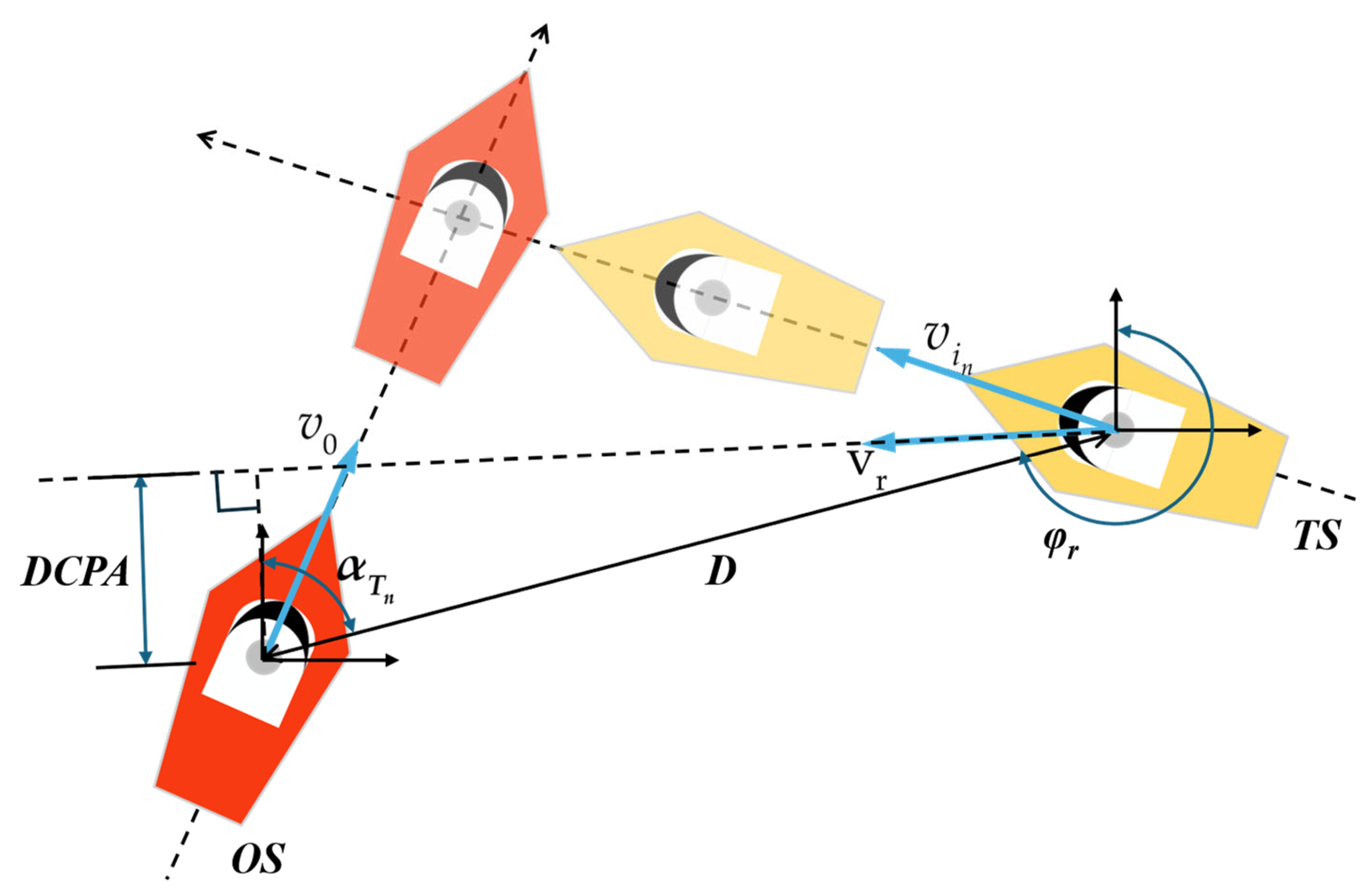
A collision risk (CR) metric is introduced into the reward function, based on the distance to the closest point of approach (DCPA) and time to the closest point of approach (TCPA). Regulations from COLREGs are integrated, and factors influencing the collision avoidance process are considered, constructing a refined reward signal tailored for training unmanned ships.

(3)

The proposed algorithm is implemented on the Unreal Engine 5 (UE5) physics engine platform, creating a simulation environment that mirrors maritime navigation characteristics. Experimental validation is conducted to demonstrate the effectiveness and practicality of the proposed method.

This study contributes a robust and compliant approach to collision avoidance in autonomous ship navigation, enhancing safety and operational efficiency in complex maritime environments.

The organization of this paper is as follows: Section 2 presents the ship dynamics model, COLREGs, collision risks, and mathematical models of ships. Section 3 covers deep reinforcement learning methods, network frameworks, PPO optimization techniques, the design of action and state spaces, and reward function design. Section 4 describes the establishment of the training environment and the presentation of training results, and it includes tests conducted on the improved ship collision avoidance algorithm within the UE5 environment. The paper concludes with a summary and outlook.

2. Problem Description

2.1. Ship Motion Dynamics

This study utilizes the mathematical models of ship dynamics proposed by Yasukawa and Yoshimura (2015) [18], Sandeepkumar et al. (2022) [19], and Sivaraj et al. (2022) [20] to construct the simulation environment, as shown in Equation (1):

$$\left\{\begin{array}{c}(m+m_x)\dot{u}-(m+m_y)vr-x_{G}m{r}^2=X_H+X_R+X_P+X_W\\ (m+m_y)\dot{v}-(m+m_x)ur+x_{G}m\dot{r}=Y_H+Y_R+Y_W\\ (I_{z}G+x_G^{2}m+J_z)\dot{r}+x_{G}m(\dot{v}+ur)=N_H+N_R+N_W\end{array}\right.$$

(1)

where $m$ represents the mass of the ship, $m_x$, $m_y$ denote the added mass in the x and y directions, $u$, $v$, $r$, $\dot{u}$, $\dot{v}$, $\dot{r}$ represent the velocities and accelerations in the x, y, and yaw directions, respectively. $I_z$ and $J_z$ represent the moment of inertia and the additional moment of inertia, respectively, along the z-axis, $x_G$ is the center of gravity along the x-axis. The hydrodynamic forces are divided into components caused by the hull ($H$), propeller ($P$), rudder ($R$), and waves ($W$).

During navigation, the ship acquires relevant parameters from other vessels and calculates collision avoidance parameters, as shown in Figure 1. The positions of one’s own ship (OS), target ship (TS), and goal are ($x_0$, $y_0$), ($x_{i_n}$, $y_{i_n}$), and ($x_g$, $y_g$), respectively. The OS’s speed is $v_0$, the blue arrow indicates the direction of speed, its heading is ${\phi }_0$, and its rudder angle is ${\delta }_0$. The target ship’s speed is $v_{i_n}$, its heading is ${\phi }_{i_n}$, its bearing relative to one’s own ship is ${\alpha }_{T_n}$, the relative bearing from OS to the goal is ${\alpha }_g$, and the distance to the nearest point on the reference path is $D_{\mathrm{r}}$.

Figure 1. Collision avoidance schematic diagram.

2.2. COLREGs

It is crucial for the development of autonomous ship collision avoidance systems to accurately understand behavioral norms under different collision scenarios and to consider maritime collision avoidance rules. Based on the COLREGs and an in-depth analysis of steering and navigation rules, we have systematically organized the collision avoidance strategies that should be followed when ships encounter other moving vessels, as shown in Figure 2, ensuring logical consistency and clear expression.

Figure 2. Collision avoidance according to the COLREGs for each situation.

(1)

Overtaking: When a ship is located within the rear quadrant of another moving ship (112.5° to 247.5°), it is in an overtaking encounter situation. If the overtaking ship is faster than the ship being overtaken, it must take appropriate measures to avoid a collision, safely maneuvering by altering course to port or starboard to pass at a safe distance between the two ships.

(2)

Head-on: When two ships are on opposing or nearly opposing courses, and the bearing of the approaching ship is within the 0° to 5° or 355° to 360° range relative to one’s own ship, it is defined as a head-on situation. In this case, both ships should alter course to starboard, passing port to port to prevent a collision.

(3)

Crossing-stand-on: If a moving ship is located on the port side of one’s own ship, within a bearing range of 247.5° to 355°, it is defined as a crossing-stand-on. In this scenario, one’s own ship, being the stand-on ship, should maintain its course and speed.

(4)

Crossing-give-way: When a moving ship is situated on the starboard side of one’s own ship, with a bearing between 0° and 112.5°, it is defined as a crossing-give-way. In this case, one’s own ship should take action to alter course to starboard to ensure a safe distance between the ships and to avoid the crossing ship.

2.3. Collision Risk

The introduction of collision risk (CR) not only simplifies the decision-making process for collision avoidance but also enhances the predictability and controllability of collision avoidance actions. The calculation of CR is based on the quantitative analysis of key parameters such as TCPA and DCPA. As shown in Figure 3, $D$ represents the distance between the two ships, ${\phi }_r$ is the relative heading between one’s own ship and the target ship, and ${\alpha }_{T_n}$ indicates the bearing of the target ship relative to one’s own ship. $v_0$, $v_{i_n}$, and ${\mathrm{v}}_{\mathrm{r}}$ denote the speed of one’s own ship, the target ship, and their relative speed, respectively. The blue arrow indicates the direction of speed. These parameters form a comprehensive risk assessment system for ship collision avoidance, providing an intuitive and reliable method to assess collision risk.

Figure 3. Concepts of DCPA, and TCPA.

The formula for calculating the distance to the closest point of approach (DCPA) between two ships is as follows:

$$DCPA=D\sin ({\phi }_r-{\alpha }_r-\pi )$$

(2)

The formula for calculating the time to the closest point of approach (TCPA) between two ships is as follows:

$$TCPA={\displaystyle \frac{D\cos ({\phi }_r-{\alpha }_r-\pi )}{v_r}}$$

(3)

To accurately assess the CR and effectively implement avoidance strategies, it is essential to consider the ship domain (SD) [21] as a critical factor. The size and shape of the ship domain directly determine the outcome of the CR assessment, defining scenarios where ships are deemed to encounter potential collision risks. Numerous methods exist for determining ship domains [22,23], ranging from complex theoretical algorithms to detailed adjustments based on expert knowledge. In this paper, we employ a circular ship domain as a simple and intuitive method, which is both practical and efficient, as shown in Figure 2, illustrating the ship domains of OS and TS with a radius, r. The circular ship domain is easy to calculate and apply, significantly simplifying operational procedures and enhancing the efficiency and accuracy of ship collision avoidance decisions. Despite its simplicity, this method offers significant advantages in navigational safety and decision-making efficiency, providing a clear approach to addressing challenges in complex maritime conditions. Therefore, the CR assessment formula designed in this paper is as follows [24,25]. The objective function to be maximized is:

$$CR=\exp \left(-{\displaystyle \frac{DCPA}{{\mathrm{c}}_1}}\right)-\exp \left(-{\displaystyle \frac{TCPA}{{\mathrm{c}}_2}}\right)$$

(4)

To determine the coefficients for DCPA and TCPA, the size and speed of the OS and the TS, as well as the operational distance at which actual collision avoidance maneuvers commence, were considered. These coefficients are set to ensure that when the TS is at the edge of the OS’s recognition distance (dr), a constant collision risk threshold, defined as allowable CR (CRal), is maintained. The dr is defined as the distance at which one’s own ship starts to identify and monitor the target ship, while the CRal is used to determine when one’s own ship should take action to avoid a collision with the target ship. To validate the effectiveness of the designed method, a KVLCC 2 tanker [26] was chosen as the example vessel. Table 1 summarizes the main parameters of this example ship.

Table 1. Principal dimensions of KVLCC2 and key parameters for collision avoidance.

Items	Value	Items	Value
Length (L)	320 m	Ship domain	900 m
Speed (V)	13 knots	Recognition distance (dr)	2000 m
Breadth	58 m	Allowable CR (CRal)	0.35
Turning radius	900 m	Coefficient 1 (c1)	1588
Max rudder angle	35°	Coefficient 2 (c2)	284

3. Collision Avoidance for Unmanned Ships Based on Deep Reinforcement Learning

In the field of machine learning, reinforcement learning (RL) is a core algorithmic paradigm focused on how agents learn through interaction with the environment to maximize cumulative rewards. Policy gradient methods are representative algorithms in this domain, which evaluate the performance of potential strategies to optimize decision-making processes. A significant advantage of these methods is their ability to directly parameterize strategies, particularly suitable for exploring high-dimensional action spaces [27,28]. However, significant changes in policy parameters can lead to performance instability in practice.

To address the challenges of policy gradient methods, researchers have developed trust region policy optimization (TRPO). The TRPO algorithm, inspired by natural policy gradients, centers on the idea of limiting the extent of policy updates to ensure gradual improvement in stability and performance. TRPO employs Kullback-Leibler (KL) divergence to control the magnitude of policy updates, thereby preventing excessively large update steps [29,30].

$$L^{\mathrm{TRPO}}(\theta )={\widehat{\mathrm{{\rm E}}}}_t\left[{\displaystyle \frac{{\pi }_{\theta }(a_t|s_t)}{{\pi }_{{\theta }_{\mathrm{old}}}(a_t|s_t)}}{\widehat{A}}_t\right]$$

(5)

where ${\pi }_{\theta }({\mathrm{a}}_{\mathrm{t}}|{\mathrm{s}}_{\mathrm{t}})$ is the probability of action ${\mathrm{a}}_{\mathrm{t}}$ under state ${\mathrm{s}}_{\mathrm{t}}$ according to the new policy. ${\widehat{\mathrm{A}}}_{\mathrm{t}}$ is the advantage function, used to assess the superiority of action ${\mathrm{a}}_{\mathrm{t}}$ compared to the average policy.

TRPO maintains stability during policy iteration by constructing a trust region, which prevents performance degradation due to overly large update steps. However, the application of TRPO often involves complex second-order optimization computations, limiting its wider application and scalability.

To address the limitations of TRPO, Schulman et al. [31] introduced proximal policy optimization (PPO). The PPO algorithm regulates the policy update process as follows:

$$L^{\mathrm{PPO}}(\theta )={\widehat{{\rm E}}}_t\left[\min \left(r_t(\theta ){\widehat{A}}_t,\mathrm{clip}(r_t(\theta ),1-ϵ,1+ϵ){\widehat{A}}_t\right)\right]$$

(6)

where $r_t(\theta )$ represents the ratio of the new policy to the old policy (importance sampling ratio). Clipping operations constrain changes in this ratio, preventing excessively large updates and, thus, enhancing the stability of the algorithm. This approach not only simplifies the implementation process but also shows significant advantages in terms of sample complexity, scalability, and performance.

PPO effectively mitigates severe fluctuations in performance that could result from policy updates by limiting the likelihood ratio between new and old policies. The implementation of PPO consists of two fundamental steps: first, executing the policy and collecting data, and second, using a gradient ascent algorithm to optimize the agent’s objective function.

In the PPO algorithm, the loss function consists of three parts: the policy objective function $L_t^{\mathrm{PPO}}(\theta )$, the value function term $L_t^{\mathrm{VF}}$, and the entropy term $H(\pi (a_t|s_t))$ [32]. These components are combined into the total loss function of PPO, where coefficients $C_1$ and $C_2$ are used to adjust the weights of the value function and entropy term. The policy objective function aims to optimize decision-making effectiveness, the value function term improves the accuracy of state estimation, and the entropy term enhances policy exploration to prevent premature convergence to local optima.

Specifically, the loss function in PPO can be expressed as follows:

$$L_t(\theta )={\widehat{\mathrm{{\rm E}}}}_t\left[L_t^{\mathrm{PPO}}(\theta )-C_1{L}_t^{\mathrm{VF}}+C_{2}H(\pi (a_t|s_t))\right]$$

(7)

where $L_t^{\mathrm{PPO}}(\theta )$ is the policy objective function, $L_t^{\mathrm{VF}}$ is the value function loss, and $H(\pi (a_t|s_t))$ represents the policy entropy, which is the entropy of the probability distribution of choosing an action, $a_t$, under a given state $s_t$ according to policy $\pi$. Adjusting $C_1$ and $C_2$ controls the influence of the value function and entropy on the total loss, balancing optimization, and exploration in the policy.

While simplifying implementation, PPO demonstrates significant advantages in terms of sample complexity, scalability, and performance. By limiting the extent of policy updates, PPO effectively avoids potential instabilities during training. Compared to TRPO, PPO simplifies the complex second-order optimization problem, thus enhancing training efficiency. However, PPO also has some limitations, such as relatively low sample utilization and sensitivity to hyperparameters, which, although less critical than in TRPO, still require careful tuning of multiple hyperparameters to ensure optimal performance.

Chaudhari and others [33] introduced entropy as a quantitative measure of randomness into the PPO objective function, increasing the uncertainty of the policy and thereby encouraging exploratory behavior. An increase in entropy implies a more exploratory policy, while a decrease leads to a more deterministic approach. In PPO, the objective function can be expressed as follows:

$$L(\theta )=L^{\mathrm{PPO}}(\theta )+\alpha \cdot H(\pi (a_t|s_t))$$

(8)

where the entropy regularization term $H(\pi (a_t|s_t))$ is added to the objective function, where $\alpha$ is a tuning hyperparameter that balances the relationship between the PPO objective function $L^{\mathrm{PPO}}(\theta )$ and the entropy regularization. Its range is from 0 to 1, with higher values encouraging more exploratory behaviors and increasing policy randomness, thereby avoiding early policy convergence. The introduction of entropy $H(\pi (a_t|s_t))$ effectively promotes exploratory behavior during policy training, especially in situations with large action spaces or complex state transitions. The introduction of policy entropy as a regularization term in the loss function helps prevent the policy from prematurely focusing on a few actions and avoids early convergence to local optima, thus motivating the algorithm to explore a wider range of state–action pairs during training. This mechanism is particularly useful in scenarios with large action spaces or complex state transitions, aiding in the discovery of better long-term strategies.

3.1. The Proposed DAE-PPO Algorithm

This algorithm optimizes the entropy regularization framework within the PPO algorithm without introducing additional hyperparameters, thus promoting more efficient exploration and improved policy performance. To further enhance the exploration capability of the policy, we propose a dynamic entropy adjustment method using a quadratically decreasing entropy approach to unify reward maximization with exploration uncertainty. This refinement allows for more precise entropy adjustments. The improved objective function incorporating the quadratically decreasing entropy term is represented as follows:

$$L(\theta )=L^{\mathrm{PPO}}(\theta )+Q(t)\cdot H(\pi (a_t|s_t))$$

(9)

Here, $Q(t)$ represents the entropy coefficient as a function of time $t$, defined as follows:

$$Q(t)={\lambda }_{\max }+({\lambda }_{\min }-{\lambda }_{\max })\cdot {\left({\displaystyle \frac{t}{t_{\max }}}\right)}^2$$

(10)

where ${\lambda }_{\max }$ represents the maximum exploration coefficient set during training, ${\lambda }_{\min }$ the minimum exploration coefficient, $t$ the current timestep, and $t_{\max }$ the total number of timesteps. The entropy coefficient decreases quadratically from ${\lambda }_{\max }$ to ${\lambda }_{\min }$ as $t$ progresses toward $t_{\max }$. This coefficient decreases quadratically over time, providing more exploration space in the early stages of training and preventing premature convergence. As training progresses, the entropy coefficient gradually diminishes, facilitating a smooth transition from exploration to exploitation and ensuring the policy quickly converges to the global optimum during the later stages of training.

The core advantage of the quadratically decreasing entropy method lies in its high entropy coefficient settings at the beginning of training, which provides ample exploration space for the model and helps prevent the strategy from converging prematurely to local optima. Compared to simple linearly decreasing methods, this approach maintains higher entropy values longer during the early training phase, thereby enhancing the breadth of policy exploration and increasing the likelihood of discovering global optima, especially in complex and variable training environments. As training progresses, the gradual decay of the entropy coefficient aids in a smooth transition to the exploitation phase, reducing training instabilities caused by sudden changes in exploration intensity. In the later stages of training, the reduced entropy coefficient encourages the strategy to utilize the knowledge acquired, thereby facilitating rapid convergence of the model and enhancing policy performance. Furthermore, the dynamic entropy adjustment method employed in this study not only improves the exploration efficiency of the PPO algorithm but also enhances the adaptability and robustness of the strategy in varied environments. With a carefully designed entropy adjustment strategy, we can more effectively guide agents in making decisions within complex reinforcement learning tasks, providing a novel optimization approach for solving practical problems.

3.2. Network Architecture and Initial Settings

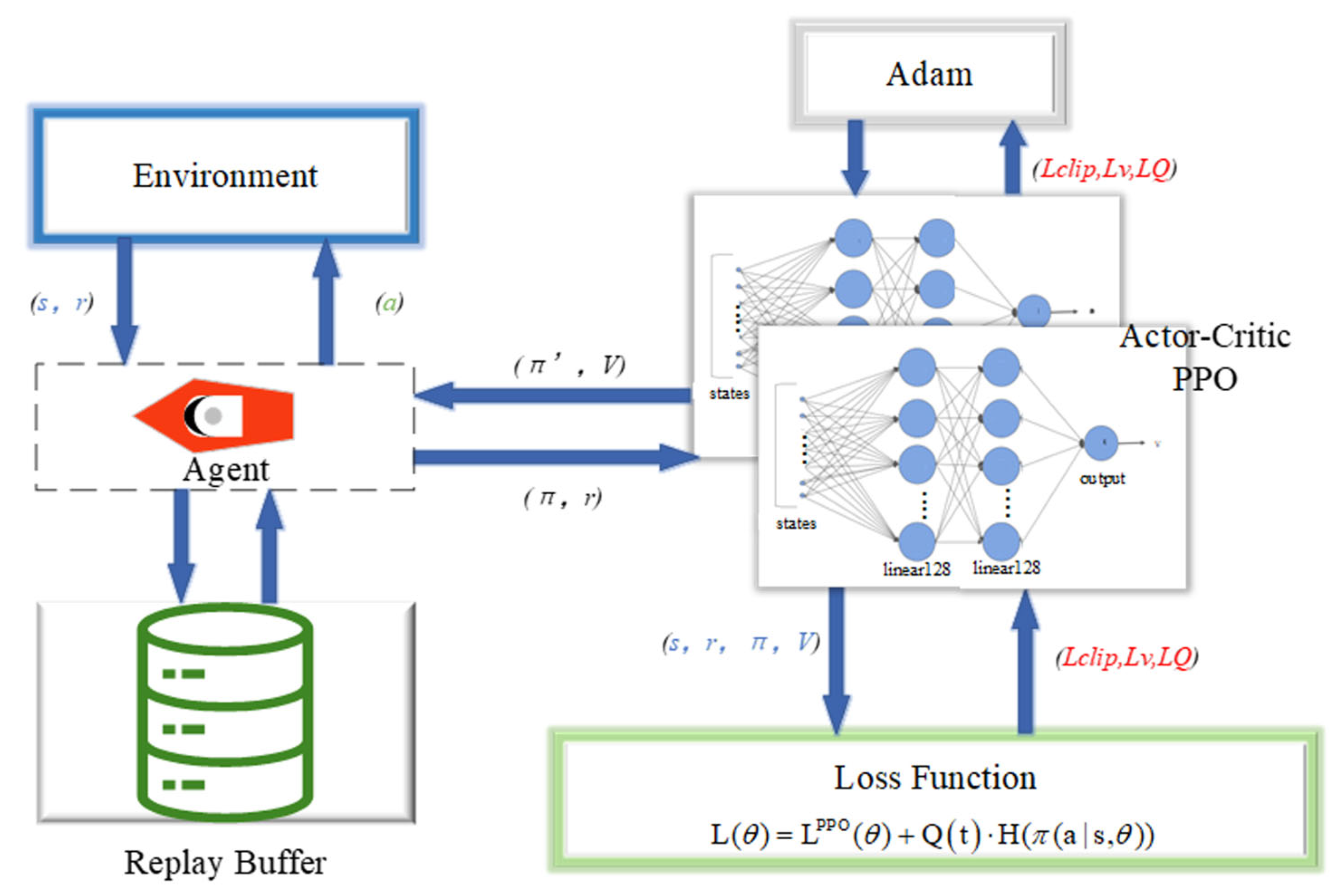
In this study, we employ an actor-critic architecture to implement the PPO algorithm, where the actor network is responsible for generating a probability distribution of actions and sampling to determine the actual actions, while the critic network estimates the state values. The dimensions of the input layer of this architecture are determined by the observation vector of the environment, while the dimensions of the output layer are dictated by the action vector. Specifically, the actor network outputs the means and standard deviations of the actions, making the output layer’s dimension twice the number of actions; conversely, the critic network outputs a single state value, with an output layer dimension of 1. In terms of hidden layer design, both the actor and critic networks employ a multi-layer perceptron (MLP) structure, with each hidden layer containing 128 units, split across two layers.

The initial steps of the training process include creating a Replay Buffer to store interaction experiences, followed by initializing the actor and critic networks, and deciding whether to use initial network weights based on the configuration file. Subsequently, both networks are configured with the Adam optimizer, and an exponential learning rate scheduler is used to adjust the learning rate.

During the training loop, experience data are received from the trainer and stored in the replay buffer. The network parameters are then updated using the PPO strategy, with the updated strategy fed back to the trainer, ensuring synchronous updates of the critic network.

The design of this network architecture aims to leverage the dual advantages of the actor-critic method: parallel optimization of policy and value functions to accelerate the learning process. The actor network’s output of action probability distributions facilitates natural policy exploration, while the introduction of entropy loss and regularization loss further incentivizes exploratory behavior, helping to prevent the strategy from prematurely converging to local optima. The critic network provides a value estimate that offers a stable reference objective for policy optimization. Furthermore, updates to network parameters are performed through a dedicated optimizer, incorporating core features of the PPO algorithm, such as clipping of probability ratios and truncation of value functions. These mechanisms work together to safeguard the update process, preventing instability due to excessively large steps.

Figure 4 illustrates the update process of the PPO algorithm. The PPO algorithm effectively captures complex feature relationships through a multi-layer perceptron structure and uses a replay buffer to store experiences, ensuring sample diversity and stability. Through clipping mechanisms and synchronous update strategies, the PPO algorithm achieves stability in policy and consistency in value estimates during training. This design not only enhances the model’s flexibility and adaptability but also ensures the robustness and reliability of the learning process.

Figure 4. Algorithm architecture.

3.3. State and Action Space Design

In the reinforcement learning framework, the environment provides the agent with observations of its current state, based on which the agent selects actions. Subsequently, the environment responds to the agent’s actions, providing feedback that includes new state information and corresponding rewards. In the context of autonomous collision avoidance tasks, unmanned ships act as agents, while obstacles, the marine environment, and other vessels constitute their environment. To ensure effective deployment and application in real-world settings, the design of the state space must closely reflect data available from actual sensors. This study has designed a multidimensional state space, as follows:

$$\begin{array}{l}S=\{{\phi }_0,{\dot{\phi }}_0,{\delta }_0,{\dot{\delta }}_0,v_0,x_0,y_0,{\alpha }_g,x_g,y_g,{\alpha }_{T_1},v_{i_1},{\phi }_{i_1},x_{i_1},y_{i_1},C{R}_{i_1},\\ \mathrm{\dots },{\alpha }_{T_n},v_{i_n},{\phi }_{i_n},x_{i_n},y_{i_n},C{R}_{i_n},D_{\mathrm{r}}\}\end{array}$$

(11)

which includes the following four parts: 1. The agent’s own navigational status: This part involves the unmanned ship’s heading, rate of heading change, rudder angle, rudder angular velocity, speed, and position coordinates, all of which collectively describe the ship’s immediate navigational state. 2. Goal-related state: This part includes the relative bearing and coordinates of the goal in relation to the unmanned ship, providing target-oriented navigation information. 3. Target ship state information: for each TS in the environment, the state space includes its true bearing, speed, heading, position coordinates, and CR relative to the OS. This information is crucial for assessing and avoiding collision risks. 4. Reference path state: this concerns the distance between the unmanned ship and the nearest point on the reference path, providing a reference for path planning and navigation.

To ensure safe navigation at sea, mariners continuously monitor collision risks and make decisions based on extensive navigation experience to make timely adjustments to the vessel’s course. Through comprehensive training in a simulation environment, the unmanned ship can learn and master these collision avoidance decision-making skills. In this study, the rudder angle serves as the action chosen by the agent through the strategy, capable of changing the unmanned ship’s direction and path.

$${\delta }_0\leftarrow {\delta }_0+{\dot{\delta }}_0$$

(12)

The rudder angle is designed in a continuous space, ${\delta }_0$ from −35° to 35°, and ${\dot{\delta }}_0$ from −5° to 5°. This design closely mimics the physical characteristics of actual ship maneuvering, enhancing the flexibility and adaptability of the unmanned ship’s navigation.

3.4. Reward Function Design

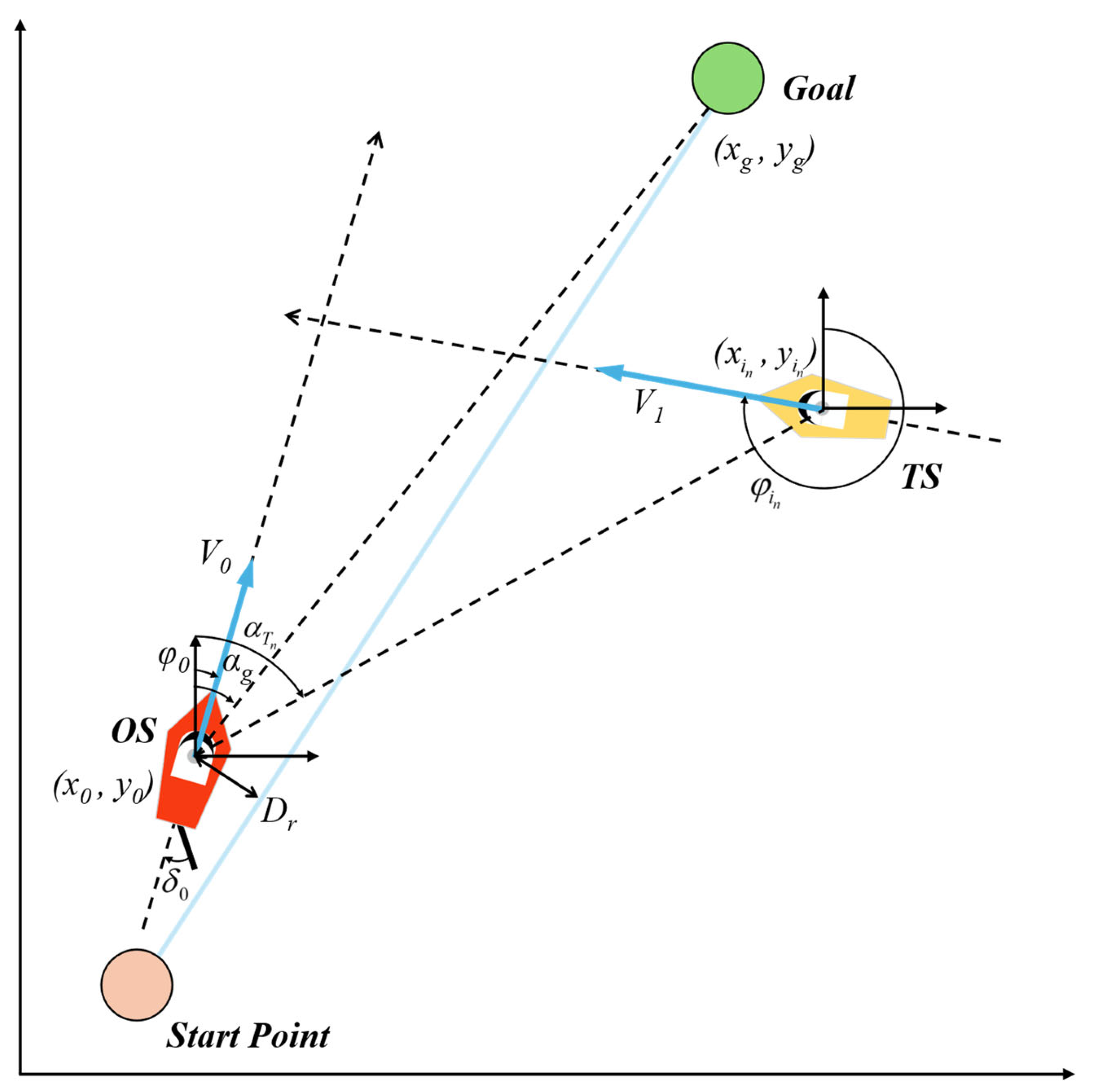
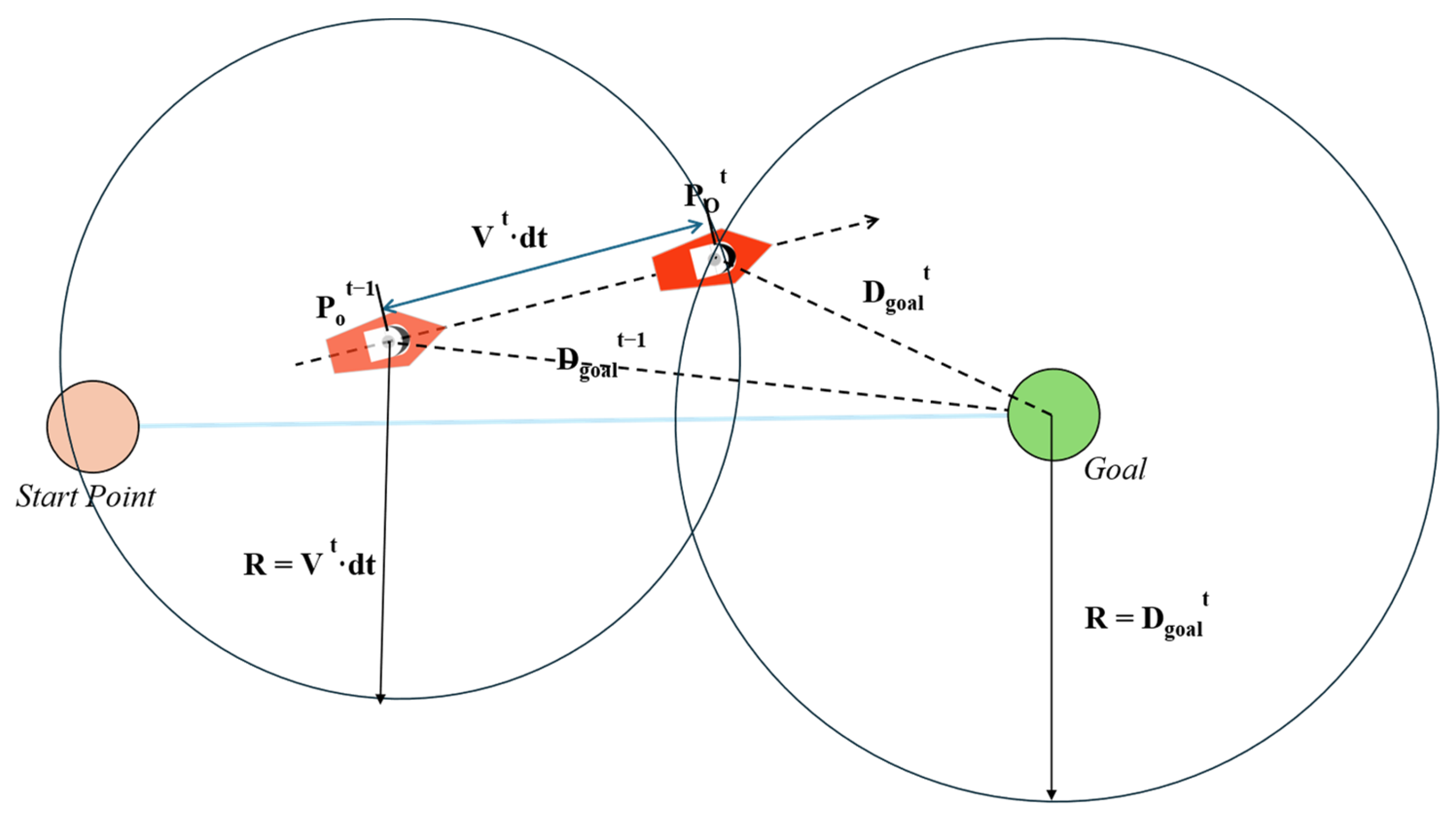
The reward function plays a crucial role in reinforcement learning, serving as a metric to evaluate the agent’s behavior and guiding the agent to act in a way that maximizes its cumulative rewards. As the training process iterates, the agent learns how to act within the explored environment to maximize its expected future benefits, eventually converging toward a stable behavior strategy. To ensure that the trained strategies effectively accomplish the autonomous collision avoidance tasks, this study divides the reward function into four components: destination reward, navigation reward, collision avoidance reward, and rule compliance reward. The reward values are calculated and accumulated at each frame. Here is the specific design of each part of the reward function:

(1)

Destination reward: This reward is designed to guide the agent toward the destination.

$$R_{goal}={\displaystyle \frac{D_{goal}^{t-1}-D_{goal}^t}{V^t\cdot dt}},D_{goal}^t=\parallel P_{goal}-P_O^t\parallel$$

(13)

where $D_{goal}^{t-1}$ and $D_{goal}^t$ are the distances between the destination and the ship’s previous and current positions, respectively. $P_{goal}$ is the goal position, and $P_O^t$ is the OS’s current position. $V^t$ is the OS’s forward speed, and $\mathrm{d}\mathrm{t}$ is the timestep. The numerator represents the difference in distance to the destination across each timestep, while the denominator represents the actual displacement of the ship per timestep. Thus, the equation effectively measures the ratio of the ship’s effective displacement toward the destination to its actual displacement. The higher the ratio, the more aligned the ship’s movement is with the direct line to the destination. Figure 5 illustrates the design principles of the reward function.

Figure 5. Navigation reward.

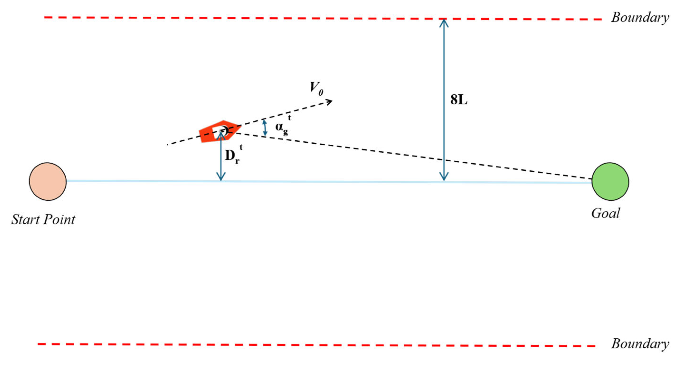
(2)

Navigation reward: This reward encourages the agent to navigate efficiently along the reference path.

$$R_{navigation}=\left\{\begin{array}{c}\begin{array}{ccc}{\displaystyle \frac{4L-D_r^t}{4L}}& if& D_r^t<8L\end{array}\\ \begin{array}{ccc}{\displaystyle \frac{90-\left|{\alpha }_g^t\right|}{90}}& if& \left|{\alpha }_g^t\right|\le 90\end{array}\\ \begin{array}{ccc}-1& if& \left|{\alpha }_g^t\right|>90\end{array}\end{array}\right.$$

(14)

where $D_r^t$ is the shortest distance between the ship and the reference path at time $t$, $L$ is the ship’s length, and the boundary distance is set to eight times $L$. The reward increases as the ship sails closer to the reference path, with the formula using four times the ship’s length as the denominator. ${\alpha }_g^t$ is the angle between the ship’s course at time $t$ and the line connecting the ship to the destination. The reward increases as the ship’s velocity direction more closely aligns with the destination. If ${\alpha }_g^t$ exceeds 90°, indicating the ship is moving away from the destination, a reward of −1 is given to discourage this behavior. Figure 6 illustrates the design principles of the reward function.

Figure 6. Simulation experiment scenes in Unreal Engine 5.

(3)

Collision avoidance reward: This reward is based on the current collision risk value and a critical threshold, aimed at preventing collisions with obstacle vessels.

$$R_{\mathrm{Collision}}=\left\{\begin{array}{ll}1\hfill & \mathrm{if} CR<C{R}_{al}\hfill \\ {\displaystyle \frac{1+C{R}_{al}-\frac{2CR}{1-C{R}_{al}}}{1-C{R}_{al}}}\hfill & \mathrm{if} C{R}_{al}\le CR\le 1.0\hfill \\ -1\hfill & \mathrm{if} 1.0\le CR\hfill \end{array}\right.$$

(15)

where $CR$ represents the current collision risk value, and $C{R}_{al}$ is the critical collision risk threshold. If $CR$ is less than $C{R}_{al}$, the ship is considered relatively safe from the target ship. If $CR$ exceeds $C{R}_{al}$, it is considered that there is a significant risk of collision, and collision avoidance decisions should be executed promptly.

(4)

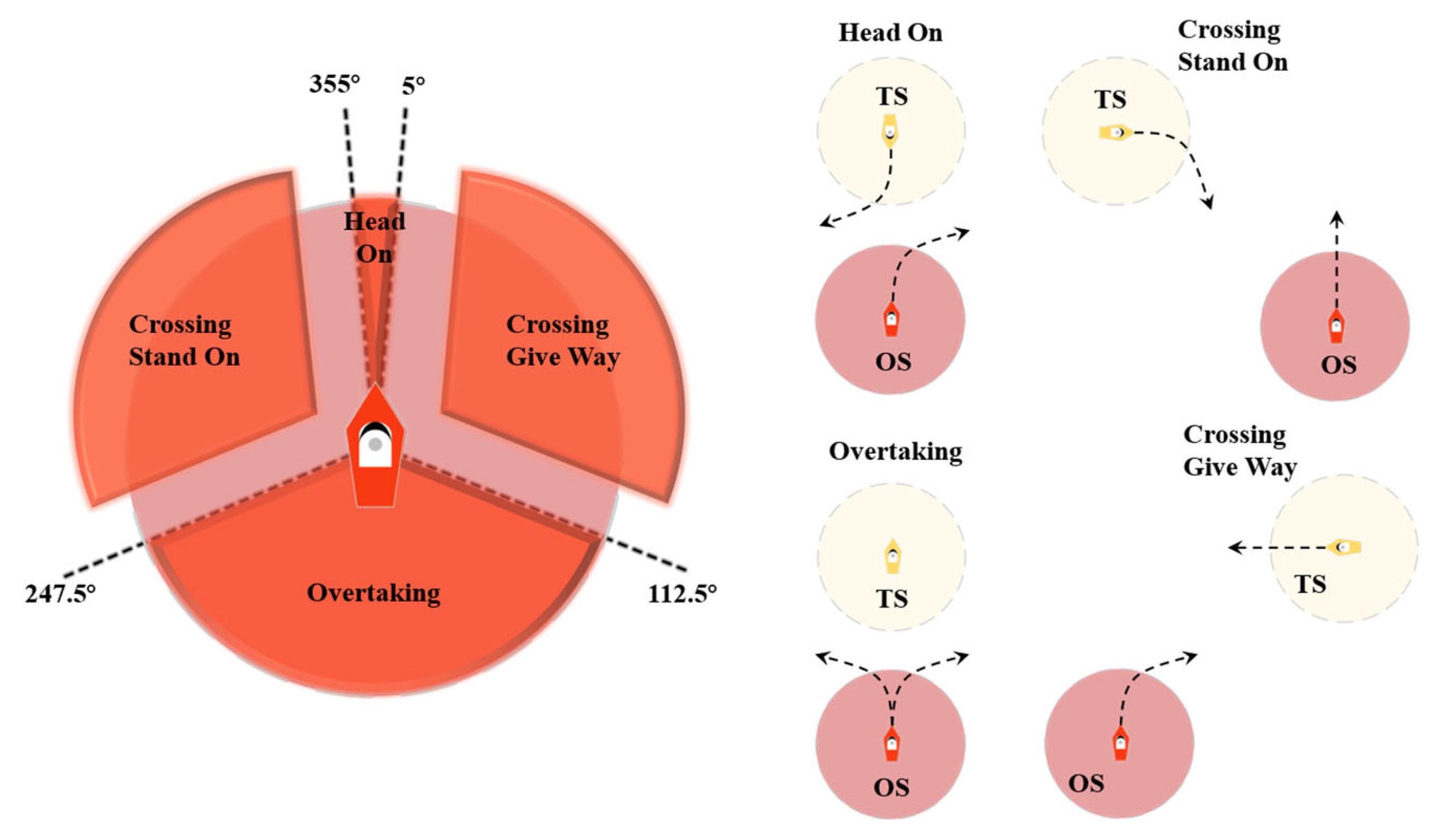
Rule compliance reward: According to the COLREGs, this reward guides autonomous ships in making collision avoidance decisions that conform to rules.

$$R_{\mathrm{COLREGs}}=\left\{\begin{array}{cc}1\hfill & \mathrm{if} \mathrm{satisfies} \mathrm{standards} \hfill \\ 0\hfill & \mathrm{otherwise}\hfill \end{array}\right.$$

(16)

COLREGs constrain the behavior of autonomous ships. First, refer to the standards in Figure 2 to assess encounter scenarios, and then determine if the OS’s decisions comply with COLREG rules 13–17 to appropriately avoid conflicts and provide corresponding rewards. If the OS decides to alter course in a head-on or starboard-crossing situation when ${\delta }_0$ > 0, it is considered compliant with COLREGs, receiving a reward value of 1; in all other cases, the reward is 0.

Through meticulous design of state spaces, action spaces, and reward functions, this study has established a comprehensive reinforcement learning training system. At each timestep, the agent’s state information is fed into the neural network, which outputs value estimates for each possible action based on current parameters and states. The agent selects the best action based on these estimates, leading to updates in the environmental state. This design ensures that the agent can learn effective collision avoidance strategies in complex maritime environments.

4. Experimental Results and Analysis

4.1. Training Environment

The simulation experiments in this study were conducted using the Unreal Engine 5.3.2 virtual simulation platform, renowned for its advanced graphical processing capabilities and physics engine. The hardware configuration of the experimental environment comprised a high-performance NVIDIA RTX 3080 GPU, customized and manufactured by ASUS, a renowned electronics company based in Taipei, Taiwan, and an Intel Core i7 4.50 GHz CPU processor, sourced from Intel Corporation, headquartered in Santa Clara, California, USA. This combination provided robust computational support for the experiments. On the software side, we utilized Python 3.7 programming language, paired with the TensorFlow deep learning framework, to construct and train our experimental models. As shown in Figure 7, we built the calm sea simulation experiment scenes in Unreal Engine 5 (UE5), ensuring the visualization and interactivity of the experiments.

Figure 7. Simulation experiment scenes in Unreal Engine 5.

As depicted in Figure 8a, for convenience, both the OS and TS are assumed to be the same ship (KVLCC2). The main specifications and parameters of the validated sample ship are summarized in Table 1. Each training session randomly generates two obstacle ships in specified states. The obstacle ships near the destination have 10 initial positions, uniformly distributed along a circular arc formed by their starting positions, with an interval β of 1° between them. This setup aims to simulate the continuity of situations that might be encountered during ship navigation. Obstacle ships near the target ship have 360 initial positions, evenly spaced by interval β along a circle formed by their starting positions. This is used to simulate various encounter scenarios. The light-colored circular area around the ship represents the ship’s domain, with a radius R closely related to the calculation of the CR value. The initial position of the target ship and its line to the destination is defined as the navigation line, which serves as an input reference for the reward function. Figure 8b shows the termination signal for the state, i.e., the end conditions for experimental training. The termination signal triggers in three scenarios: if the target ship collides with an obstacle ship, deviates beyond the maximum allowed distance from the planned route, or reaches the destination, at which point the system marks the training session as “Done”.

Figure 8. Training environment. (a) Training scene generation; (b) training termination conditions.

4.2. Algorithm Hyperparameters

Based on comprehensive considerations of the algorithm architecture and simulation environment, the selected training hyperparameters are presented in Table 2. The learning rate critic is the learning rate used to update the value function (managed by the critic network). An appropriate learning rate is crucial for ensuring the stability of the training process. The learning rate policy refers to the learning rate of the policy network, which adjusts the agent’s behavior in response to environmental feedback. The magnitude of this learning rate directly influences the dynamics of training. The learning rates for the actor and critic networks are 0.001 and 0.01, respectively. The learning rate decay is set to 0.99, which causes the learning rate to exponentially decay as training progresses, aiding in model convergence and reducing the risk of significant weight updates in the later stages of training. In the entropy-inclusive PPO algorithm, the entropy coefficient is set to 0.05, which quantifies the randomness of the strategy and encourages exploratory behavior. Its optimal value was determined through a series of debugging experiments. In the DAE-PPO algorithm, the entropy coefficient start and entropy coefficient end are set to 0.09 and 0.01, respectively, to facilitate dynamic entropy adjustment during training. Epsilon Clip (ε-Clip) is set at 0.2 to limit the magnitude of policy updates, preventing training instability due to overly large updates. Lambda (λ) is set at 0.95 to adjust the variance and bias in the generalized advantage estimation (GAE), ensuring the stability of value estimates.

Table 2. Hyperparameters for training.

Hyperparameter	Value
Learning rate critic	0.01
Learning rate policy	0.001
Learning rate decay	0.99
Entropy coefficient (entropy-PPO)	0.05
Entropy coefficient start (DAE-PPO)	0.09
Entropy coefficient end (DAE-PPO)	0.01
Epsilon clip	0.2
Lambda (GAE)	0.95
Discount factor (γ)	0.99

4.3. Training Process

Figure 9 shows the trends in average reward values and the corresponding confidence intervals for three algorithms over 20,000 training episodes. The red curve represents the PPO algorithm with dynamically adjusted entropy (DAE-PPO), the green curve represents the entropy-inclusive PPO algorithm, and the blue curve represents the classic PPO algorithm. The shaded areas in the graph indicate the confidence intervals for each algorithm. In the early stages of training, DAE-PPO has a wider confidence interval, indicating that the algorithm adopts a broader exploration strategy initially. This strategy helps the algorithm quickly identify behavior patterns that yield higher rewards. As training progresses, after about 5000 episodes, the average reward for DAE-PPO begins to significantly increase, and its confidence interval starts to narrow, demonstrating the algorithm’s performance stability. By 8000 training episodes, the average reward for DAE-PPO stabilizes and ultimately reaches a high level. The DAE-PPO algorithm, by employing a quadratic decay interpolation of entropy, demonstrates significant advantages in autonomous ship navigation and collision avoidance tasks. This entropy decay strategy optimizes the balance between exploration and exploitation, not only enhancing the algorithm’s average reward but also its stability and reducing convergence time. In contrast, both the traditional PPO algorithm and the entropy-inclusive PPO algorithm have not surpassed DAE-PPO in terms of reward values and stability, thus confirming the superiority of DAE-PPO in such tasks.

Figure 9. Average reward.

Figure 10 provides a visual display of the agent’s performance across various training stages, offering a detailed tracking and evaluation of the entire learning process.

Figure 10. Training. (a) First episode; (b) 1432nd episode; (c) 3646th episode; (d) 5600th episode; (e) 7763rd episode; (f) 9981st episode.

Figure 10a shows the agent’s training in the first episode. Due to the random initialization of neural network parameters and the agent’s unfamiliarity with the environment, its movement is based on random exploration, leading to circling behavior at the starting position.

Figure 10b displays the agent’s training in episode 1432. The agent learns from feedback that circling at the initial position is not a reward-driven behavior, thus it begins to explore the scenario. It then collides with an obstacle ship and the training ends. Although this training session failed, the interaction experience is crucial for future exploration.

Figure 10c illustrates the training effect in episode 3646, where the agent successfully avoids ST2 and begins to try more behaviors to explore the scenario.

Figure 10d shows the training outcome in episode 5600, where the agent’s behavior aligns more closely with the intended guided rewards. The failed experience of colliding with obstacle ship ST1 is essential for achieving better training results.

Figure 10e presents the training result in episode 7763, where the agent meets basic collision avoidance requirements and reaches the destination for the first time, validating the design of the guided rewards.

Figure 10f depicts the training result in episode 9981, where the agent’s behavior has become largely stable and efficient, gradually meeting the expectations.

4.4. Results Analysis

From the reward curve graph in Figure 9, it is evident that after completing 20,000 training cycles, all three algorithms have reached a state of convergence. In particular, the DAE-PPO demonstrates significant advantages in terms of convergence speed, stability after convergence, and average rewards post-convergence, surpassing the other two algorithms. To further visually demonstrate the performance advantages of the improved algorithm after model convergence, this paper specifically selects a typical encounter scenario to conduct comparative tests among the three algorithms.

As shown in Figure 11a,b, the initial positions of OS, TS1, and TS2 are (6117.98, 1863.74), (4832.98, 4510.49), and (687.41, 7271.13), respectively, with the obstacle ships maintaining constant speed and course. Figure 11a,b, respectively, show the trajectory and the relative distance curves of the OS and TS for the classic PPO training model. The classic PPO model exhibits significant fluctuations in ship heading, showing a lack of stability, and the closest distances to TS1 and TS2 are both less than 600 m, indicating a high risk of collision. Moreover, the decision-making during encounters does not comply with the COLREGs.

Figure 11. Encounter situation. (a) Path planned by classic PPO; (b) distance curve between OS and TSs for classic PPO; (c) path planned by entropy-PPO; (d) distance curve between OS and TSs for entropy-PPO; (e) path planned by DAE-PPO; (f) distance curve between OS and TSs for DAE-PPO.

Figure 11c,d present the trajectory and the relative distance curves of the OS and TS for the entropy-PPO training model. Compared to the classic PPO model, the entropy-PPO model’s course is more stable, maintaining a higher safety distance with TS, yet the closest point remains at a fairly close 604.64 m. Actions during encounters with TS1 and TS2, such as turning left too little or lacking clear movement, do not comply with COLREGs.

Figure 11e,f showcase the trajectory and relative distance curves of OS and TS for the DAE-PPO training model. The trajectory indicates that DAE-PPO exhibits greater stability in collision avoidance decisions compared to the previous two models. The encounter decisions comply with COLREGs and are clearly and succinctly executed. As seen in Table 3, the DAE-PPO algorithm performs excellently in collision avoidance, with the widest separation and the lowest collision risk among the algorithms, and it achieves this in the shortest time of 135 s, indicating its strong capability in complex encounter scenarios.

Table 3. Results of collision avoidance of Example.

Algorithms	Minimum Distance between Ships [m]	Maximum Collision Risk	Time
DAE-PPO	777.05	0.72	135
Entropy-PPO	604.64	0.81	137
Classic PPO	508.65	1.07	159

To verify the generalization ability of the algorithm, 100 sets of random experiments were conducted under the same random seed. In the same environment, 100 collision avoidance tests were conducted, with the number of successful incidents recorded. As shown in Table 4, the DAE-PPO algorithm significantly outperformed other algorithms in terms of success rate in multiple experiments, further validating its stability and reliability.

Table 4. Results of 100 times experiments.

Algorithm	DAE-PPO	Entropy-PPO	Classic PPO
Successful arrival	96	81	51

Figure 12 displays a challenging encounter scenario involving three obstacle ships, designed to assess the performance of collision avoidance models in handling complex situations.

Figure 12. Collision avoidance environment. (a) Path planned; (b) distance curve between OS and TSs.

In this scenario, the initial positions of OS are (6121.76, 1857.45), with TS1, TS2, and TS3 starting at (4654.17, 4721.57), (−928.20, 8911.22), and (1458.61, 3880.10), respectively. During the simulation, the course and speed of the obstacle ships remain constant. Figure 12a shows the completed path of OS. When OS and TS1 formed a crossing-give-way situation with a potential collision risk, the agent made a significant right turn. The minimum distance between the two ships was recorded as 766.25 m, successfully achieving safe avoidance, and the decision strictly followed the COLREGs. After the avoidance maneuver, OS corrected its rudder angle and, after a stable course, performed a crossing-stand-on encounter with TS3. At this point, the agent decided to turn left. During this process, the minimum distance between the two ships was 1098.60 m. After avoiding TS3, OS continued to navigate smoothly toward the destination. Subsequently, OS and TS2 encountered a head-on situation. OS quickly made a significant right turn, and during this process, the minimum distance between the two ships was again 1098.60 m, with the avoidance behavior also complying with COLREGs. After completing the avoidance, OS began to resume its course and smoothly reached its destination.

Through this simulation, we validated the effectiveness and compliance of the collision avoidance model in handling complex maritime traffic scenarios, ensuring safe and compliant navigation in varied maritime environments.

5. Conclusions

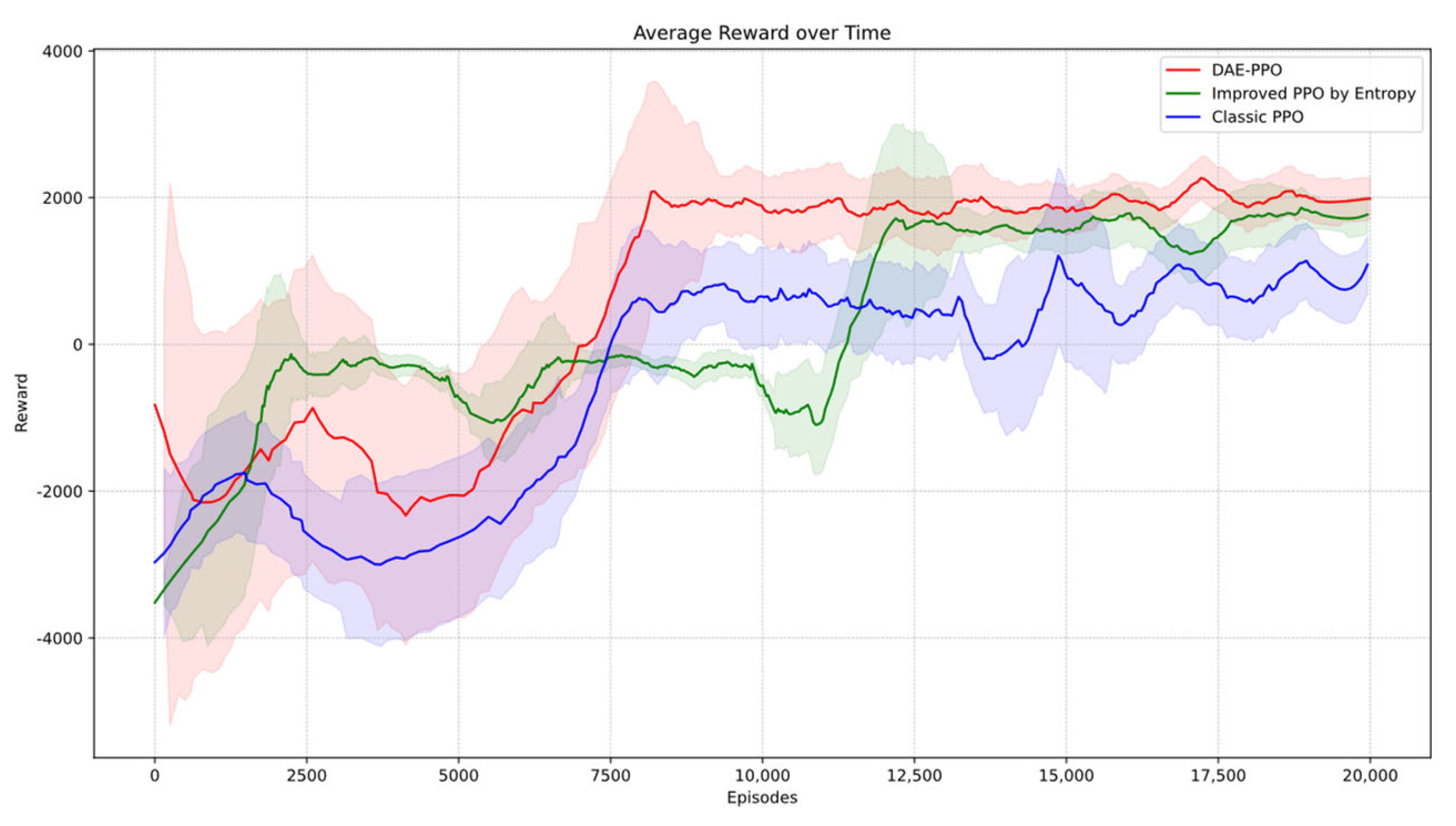
This study addresses the issue of ship collision avoidance in maritime transport environments by proposing an improved PPO algorithm (DAE-PPO) based on dynamically adjusted entropy. The algorithm optimizes the exploration mechanism through a quadratically decreasing entropy method, effectively avoiding local optima and enhancing strategic performance, all while considering the COLREGs. Simulation results indicate that the DAE-PPO algorithm significantly outperforms in efficiency, success rate, and stability in collision avoidance tests.

Moreover, the reward function designed in this study is subdivided into destination, navigation, collision avoidance, and rule compliance rewards, effectively guiding the agent in making effective collision avoidance decisions in complex maritime environments.

Despite the significant achievements of the DAE-PPO algorithm in simulated environments, future research needs to delve deeper into several areas: While simulation environments can emulate various scenarios, the complexity and unpredictability of actual maritime environments are higher. Future work should include testing and validating the algorithm in real maritime conditions. Maritime traffic often involves interactions among multiple ships; research could explore collaborative collision avoidance strategies within multi-agent systems to enhance the efficiency and safety of overall maritime traffic. The exploration of elliptical ship domain models, which can dynamically adjust based on the speed of unmanned ships, will more accurately simulate real-world collision avoidance scenarios. Through these subsequent studies, we will aim to further enhance the performance of autonomous collision avoidance algorithms for unmanned ships, advance unmanned ship technology, and ultimately achieve safe and efficient autonomous maritime navigation.