Article

A Comprehensive Investigation of Linear and Nonlinear Beam Models on Flexible Wind Turbine Blade Load Calculations

1
College of Engineering, Shantou University, Shantou 515063, China
2
Key Laboratory of Intelligent Manufacturing Technology (Shantou University), Ministry of Education, Shantou 515063, China
3
Housing and Urban-Rural Development Bureau of Huizhou Huiyang District, Huizhou 516007, China
4
School of Electric Information and Electrical Engineering, Huizhou University, Huizhou 516007, China
*
Author to whom correspondence should be addressed.
J. Mar. Sci. Eng. 2024, 12(4), 548; https://doi.org/10.3390/jmse12040548
Submission received: 5 March 2024 / Revised: 20 March 2024 / Accepted: 22 March 2024 / Published: 25 March 2024
(This article belongs to the Topic Wind, Wave and Tidal Energy Technologies in China)

Abstract

:
This study was performed to investigate the effects of structural nonlinearity and large deformations on the aeroelastic loads of flexible wind turbine blades. First, a blade structural analysis model was established using the geometrically exact beam (GEB) theory. Subsequently, the blade element momentum (BEM) theory was corrected using the geometrically exact method leading to the development of a geometrically exact blade element momentum (GE-BEM) model. The results from the GE-BEM model indicated that flapwise deformations always reduce blade fatigue loads, while torsional deformations decrease fatigue loads under low wind speeds but increase them under high wind speeds. Finally, the linear Euler–Bernoulli beam and the GEB were compared to explore the influence of geometric nonlinearity on the blade aeroelastic loads, which revealed that the Euler beam model underestimates the blade loads. The simulations that used the GEB model produced torsional root twist fatigue loads that were 57.49% greater than those generated when the Euler beam model was used. Furthermore, the flapwise bending moment fatigue loads at the root were 8.24% greater than those obtained by the Euler beam model. The smallest discrepancy between the results of the two models was 7.26%, and it corresponded to the edgewise fatigue load.

1. Introduction

The trend toward the upscaling of offshore wind turbines by increasing their sizes and capacities is intricately linked with the widespread development of global offshore wind farms. Technological advancements, particularly those regarding the utilization of maritime transport, have effectively addressed the logistical challenges associated with transporting large wind turbine components. These advancements have enabled the design and manufacture of turbines on a larger and more flexible scale. Driven by economic considerations, the global offshore wind power industry is progressively adopting higher-capacity turbines to enhance the unit power output instead of adding more small units. These colossal offshore wind turbines feature larger, longer, and more flexible towers and blades than previously used turbines [1]. For example, the mean rated power capacity of the offshore wind turbines installed in Europe in 2023 was 9.7 MW, which represents a 1.7 MW increase from those installed in 2022 [2]. Chinese wind energy enterprises have successfully installed offshore wind turbines with blade lengths that reach 123 m and that have nominal capacities of 16 MW [3]. On 10 November 2023, the Dongfang Electric Corporation completed an 18 MW offshore wind turbine with a blade length of 126 m [4]. Projections for the year 2030 predict the emergence of offshore wind turbines with rotor diameters of 250 m and power capacities of 20 MW [5,6].
As the development of larger wind turbines has progressed, turbine blades have become increasingly slender, and the turbine structures have grown increasingly intricate. In addition, to enhance their aerodynamic performance, blades are frequently designed with pre-bend, pre-twist, and pre-sweep characteristics. The blades are designed to withstand substantial deformations, which can passively reduce the loads and enhance the aerodynamic performance. The traditional aeroelastic methods, which assume that the blades are either rigid or undergo small deformations, are no longer reasonable. Modern blades typically have tip deflections that range from 3% to 10% of the blade length [7], though deformations equal to 15% to 20% of the blade length can occur under extreme wind conditions [8]. Under normal operating loads, the blade structural deformations of modern large wind turbines have surpassed the limits under which small deformation assumptions are applicable and have exhibited pronounced nonlinearity. Traditional linear beam models that are based on small deformation assumptions are inadequate for accurate blade deformation analyses [9]. Moreover, significant blade deformations influence the aerodynamic shapes and load distribution. The vibrations that result from substantial blade oscillations affect the inflow velocity of the wind, thereby significantly impacting the aerodynamic loads; this phenomenon is known as the aeroelastic effect [10]. Blade aeroelasticity analyses cannot disregard the aeroelastic loads induced by these effects [11,12]. The challenges associated with these aeroelastic effects, which originate from nonlinear blade deformations, have spurred extensive research. Scholars have explored the aeroelasticity problems associated with wind turbine blades by approaching the issue from the following two perspectives: unsteady aerodynamics and nonlinear structural dynamics.
Several methods are commonly used to perform aerodynamic calculations for wind turbines. These methods, which are listed according to increasing computational precision but decreasing computational efficiency, include the blade element momentum (BEM) model, the vortex model, the actuator-type model, and the computational fluid dynamics (CFD) method [13]. Despite the pursuit of advanced methodologies to refine wind turbine aerodynamics calculations, engineering models that use the BEM method persist as the dominant aerodynamic models utilized by mainstream wind turbine simulation software, such as DNV Bladed, FAST, CP-Lambda, hGAST, and HAWC2 [13,14]. Consequently, researchers have persistently focused on enhancing BEM models to augment computational precision. Zhong et al. (2019) [15] used the CFD method to investigate the flow fields near rotating turbine blades and proposed an innovative methodology for ascertaining the effective angle of attack for individual blade elements within the BEM model. Sun et al. (2016) [16] refined the generalized momentum theory by incorporating considerations for radial flow and improved the wind speed accuracy of the BEM model. Fritz et al. (2022) [17] investigated the influence of aft-swept blades on aerodynamic performance and proposed refinements to the BEM methodology. They found that aft-swept geometries result in a reduced axial induction, particularly around the tip. Sayed et al. (2019) [18] conducted a comparative analysis of aerodynamic loads calculated by both the engineering BEM and CFD methods; their results revealed a tendency for engineering models to underestimate power and thrust. Rezaei et al. (2015) [19] employed a nonlinear geometrically exact beam (GEB) model to represent a turbine blade; the results of this model then served as feedback to an aerodynamic model, which fully incorporated the effects of rotor deformation into the aerodynamic load calculations. Liu et al. (2017) [12] examined unsteady aerodynamic blade loads under dynamic stall conditions by incorporating vibration velocity feedback into the blade aerodynamic model; in their study, they utilized a combination of the BEM model and the Beddoes–Leishman dynamic stall model. In summary, increasing computational accuracy by continually refining the BEM method persists as a pivotal means of addressing engineering and technical challenges present in wind turbine technology.
Common methods of approaching wind turbine structural dynamics calculations include the 3D finite element method and the 1D equivalent beam element method [20]. The existing 1D equivalent beam element models can be broadly divided into linear and nonlinear models. The Euler–Bernoulli and Timoshenko beam models are typical examples of linear beam models. Both the Euler–Bernoulli and Timoshenko beam models rely on the small deformation assumption and are not applicable to wind turbine blades that experience substantial deformations. A frequently employed alternative that is used when there are large deformations is the GEB model [13]. The 3D finite element method is typically investigated using commercial finite element analysis software, such as ANSYS or ABAQUS [21]. Many scholars are dedicated to enhancing both the aerodynamic and structural models of wind turbines while simultaneously conducting coupled analyses, known as aeroelastic analyses. The goal of these studies is a comprehensive understanding of the aeroelastic characteristics of wind turbines, which can enable the design of more efficient and reliable wind turbines. Early efforts primarily focused on achieving structural–aerodynamic coupling and an understanding of how structural vibration feedback influences aerodynamic models. Wang et al. (2014) [9] and Li et al. (2020) [7] conducted aeroelastic analyses of flexible blades using the GEB method coupled with the BEM method. They demonstrated that the GEB method can more accurately describe large vibration deformations of flexible blades. Utilizing a large eddy simulation solver and a linear beam model, Della Posta et al. (2022) [22] conducted a coupled analysis of wind turbine aerodynamics and structural dynamics, specifically examining the influence of blade torsional vibrations on aeroelastic loads. Mo et al. (2015) [23] proposed an aeroelastic simulation program based on flexible multibody dynamics and combined the BEM method with a dynamic stall model. Sabale and Gopal (2019) [24] utilized the GEB and BEM methods, while accounting for dynamic stall, to establish an aeroelastic analysis model. Using both multibody dynamics and GEB models in hGAST software, Panteli et al. (2022) [25] conducted a comparative aeroelastic analysis that revealed a significant disparity between the aeroelastic load calculation results of linear and nonlinear structural models. Finnegan et al. (2021) [26] compared three FEM numerical models and found that models based on “layered solid elements” give a higher accuracy in FE prediction. Manolas et al. (2015) [7] conducted a study that compared a second-order nonlinear beam model, a multibody model, and a first-order linear beam model for wind turbine blades; they found that the bending–torsional coupling effect was the primary nonlinear effect that caused differences between the loads.
Figure 1 presents calculation results from three wind turbine simulation software packages (GAST, HAWC2, and CP-Lambda) and a computational structural dynamics model (FLOWer-EMPIRE-Carat++) for blade tip deflection in the flapwise direction for a 10 MW reference wind turbine (RWT) [27]. The maximum flapwise tip displacement reached 0.125 of the blade length, which is nearly 11.1 m, at a wind speed of 11.4 m/s. As calculated by Panteli et al. (2022) [25], when the tip displacement reached 11.1 m, the tip deflection angle in the flapwise direction was −0.61 rad, while it was 0.031 rad in the torsional direction. The flapwise rotation caused the blade elements at the blade tip to experience horizontal wind speed reductions of nearly 18%. According to the momentum theorem, the thrust of a wind turbine is proportional to the square of the horizontal wind speed. Consequently, this horizontal speed reduction produced a decrease in thrust of approximately 32%. Furthermore, the 0.025 rad blade twist deflection reduced the angle of attack and significantly decreased the lift coefficient. These estimates are preliminary, and when other factors, such as the wind turbine diameter reduction caused by blade bending and the unsteady aerodynamic characteristics of the blades, are included, the blade aeroelastic load calculations become more complex. The effects of blade vibration and deformation on the aeroelastic loads cannot be overlooked. In practical engineering applications, more accurate load calculations performed under a variety of operating conditions would contribute to an improvement in blade design and control precision [10,14,28]. Even though meaningful research has been performed by scholars regarding the aerodynamics, structural dynamics, and aeroelastic coupling involved in wind turbine calculations, the mechanisms through which wind turbine deformations affect aerodynamic loads must be further explored. The process of using structural deformation information to modify the BEM model in aeroelastic coupling analyses also requires further investigation. Both qualitative and quantitative analyses are also needed to reveal the effects of structural nonlinearity on the aeroelastic loads of the blades. It was previously stated that the BEM model is characterized by high computational efficiency and precision that meets engineering requirements and that its usage is widespread. Since this study involved extensive simulations of wind turbines operating under a variety of wind conditions for extended periods of time, the BEM model was chosen for use because of these advantages. The GEB model establishes an inherent relationship between displacement and strain, thereby enabling the calculation of blade deformations across any range as well as an accurate representation of the geometric nonlinearity of the blades. Therefore, the BEM and GEB models were coupled for the aeroelastic time-domain simulations of wind turbine blades conducted during this study.
In this study, to investigate the effects of significant deformations on the aerodynamic loads of wind turbine blades, a GEB model was first employed to characterize the blades. This model achieved precise structural modeling of the position, velocity, orientation, and torsional deformation of each blade element. An accurate description of the wind speed at each blade element was obtained through precise coordinate transformations. Blade deformation and vibration speed corrections were introduced into the BEM model and a local planar assumption was adopted for the deforming rotor plane. A precise geometric correction method for the BEM model, referred to as the GE-BEM model, was also developed. This GE-BEM model accounts for variations in the wind speed at the blade elements due to blade vibrations as well as for changes in the attack angle caused by torsional oscillations. To investigate the effects of structural deformations and unsteady aerodynamic characteristics on wind turbine blade loads, different correction conditions were applied in an aeroelastic simulation model. Comparative analyses of results from aeroelastic simulation models with different correction conditions were conducted. Finally, extensive aeroelastic wind turbine simulations were performed using both the Euler beam and GEB methods coupled with the GE-BEM model, after which the simulation results were subjected to fatigue analyses. The impacts of structural nonlinearity on the blade loads were studied by comparing damage-equivalent load results from simulations performed with the Euler beam and GEB models.
This paper is organized into three additional sections. The blade structural model, which is based on the GEB method, a corrected BEM model (the GE-BEM model), and an aeroelastic simulation model, are described in Section 2. Verifications of the structural, aerodynamic, and aeroelastic models, as well as the effects of deformations and structural nonlinearity on aeroelastic loads, are summarized in Section 3. This study’s conclusions are presented in Section 4.

2. Methodology

This section presents a detailed description of the aeroelastic simulation model developed during this study. The coordinate systems required for the aeroelastic simulations and the transformation relationships between them are primarily introduced in Section 2.1 and Section 2.2. An orthogonal transformation matrix is introduced for the coordinate transformations. The GEB theory and how it is applied to the modeling of wind turbine blades is discussed in Section 2.3. The GE-BEM aerodynamic calculation model and its corrections are the focus of Section 2.4. The methods used to calculate the non-aerodynamic loads on the blades are detailed in Section 2.5. Finally, Section 2.6 explains how the structural and aerodynamic models are coupled in the aeroelastic coupling simulations and provides a discussion of coupling methods.

2.1. Orthogonal Transformation Matrix

When characterizing the beam section orientation when applying the GEB model, performing wind speed calculations for the blade elements in the GE-BEM model, and conducting load transformations among different frames in aeroelastic simulations, the coordinate transformations must be handled with precision. An orthogonal transformation tenser, , and a corresponding matrix, R, were employed for this task. They must satisfy the relationship presented in Equation (1):
R : 3 3 R T R = R R T = I ;   det R = 1
where R belongs to the Lie group of proper orthogonal linear transformations, SO(3). If Ej and tj represent the material frame and the body-fixed motion frame, respectively, their relationship to one another can be expressed by Equation (2):
t j = R E j ,   or   = t j E j . .
R is the orthogonal matrix of transformation, and it can be regarded as the rotation required to move from the initial configuration to the actual configuration. R also can be understood to represent the coordinates of the rotated basis vectors in the spatial frame. R is often defined in a special frame; however, this representation is not unique and is dependent on the frames. Various parameterization methods can be used to characterize R, such as Euler angles, quaternion, Euler parameters, and rotational pseudovector methods. However, using the rotation vector to represent R is simple and intuitive; this method is also widely employed in kinematic descriptions and coordinate transformations. It was chosen for use in this study, and is expressed by Equation (3):
Ψ = [ ψ x , ψ y , ψ z ] T . .
The magnitude, Ψ , represents the rotation angle, and its direction is the direction of the rotation axis. ψ x ,   ψ y   and   ψ z its components. The choice of using a rotation vector to represent R has some disadvantages, however, such as singularity when Ψ = π . The following revision was therefore developed and used during this study when Ψ > π : Ψ = ( 1 2 π Ψ ) Ψ . According to the Rodrigues formula [29], R can be expressed by Equation (4):
R ( Ψ ) = I + sin Ψ Ψ Ψ ˜ + 1 2 sin ( Ψ / 2 ) Ψ / 2 2 Ψ ˜ 2 ,
where Ψ ˜ is the skew-symmetric matrix formed by the components of Ψ , which are presented in Equation (5):
Ψ ˜ ij = ε ijk Ψ k , Ψ i = 1 2 ε ijk Ψ ˜ jk . .

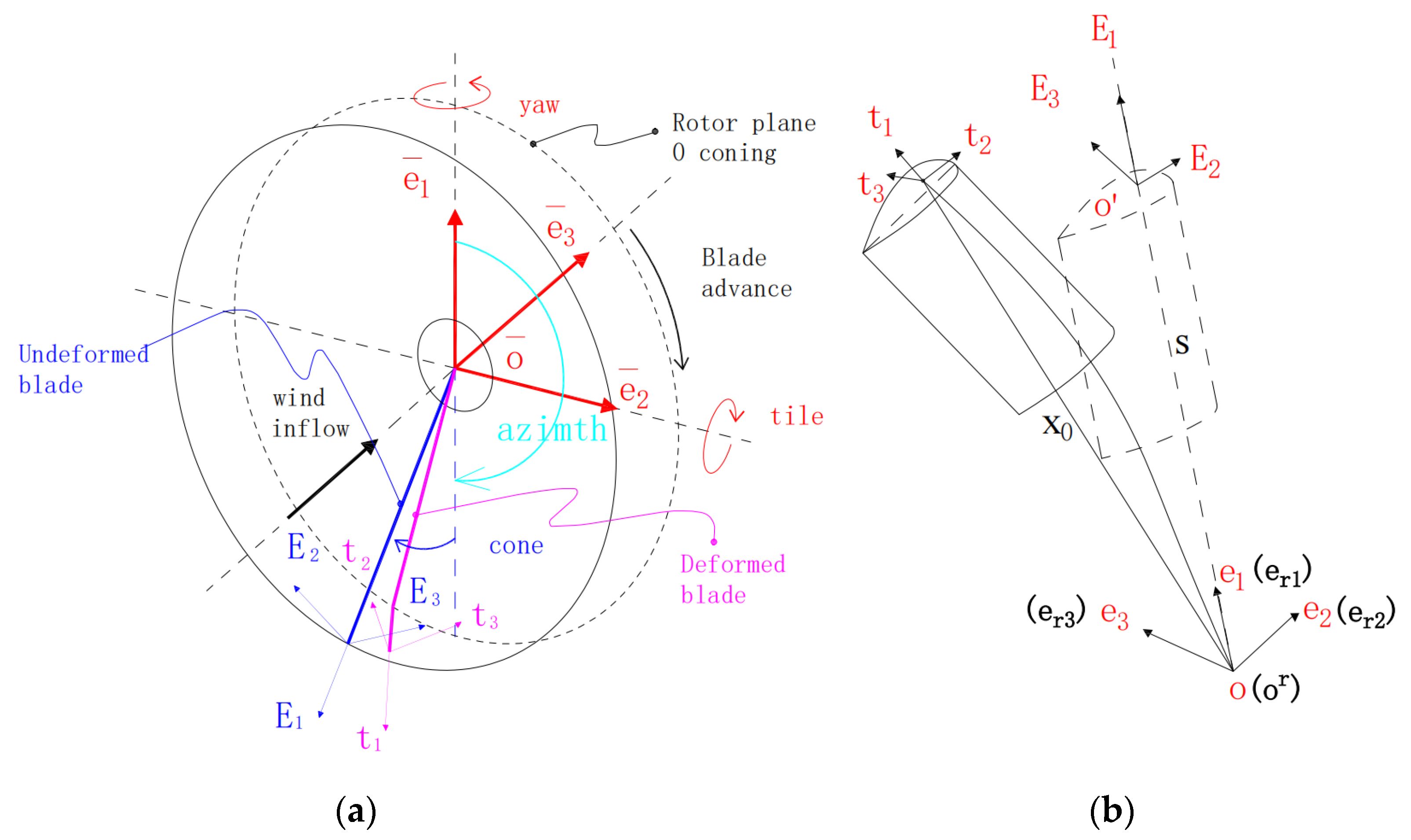
2.2. Coordinate Frames and Transformations

To accurately calculate the wind speed, rotational speed, and position of a single blade element, it is necessary to establish different frames at various locations on the wind turbine. To achieve structural–aerodynamic coupling analyses, i.e., aeroelastic analyses of the blade, it is essential to exchange vibration velocities, deformations, and load data within a unified frame. Different frames were established during this study, and transformations between these frames were conducted using the orthogonal transformation matrix discussed in Section 2.1. The definitions of the different coordinate systems, which are illustrated in Figure 2a, are provided in the following list:
(1)
First, a global inertial Cartesian frame, e ¯ j o , e ¯ 1 , e ¯ 2 , e ¯ 3 , was established, in which e ¯ 1 is oriented vertically upward and e ¯ 3 aligns with the horizontal component of the incoming wind velocity.
(2)
The nacelle frame, E nj o n ; E n 1 , E n 2 , E n 3 , was constructed by rotating the global frame, e ¯ j o ; e ¯ 1 , e ¯ 2 , e ¯ 3 , about e ¯ 1 by the yaw angle, θ yaw , then rotating it in the new frame about e ¯ 2 by the tilt angle, η. The transformation relationship can be expressed by E nj = R η R yaw e ¯ j , where R yaw = R θ yaw , 0 , 0 T   and   R η = R 0 , η , 0 T .
(3)
The hub frame, E hj o h ; E h 1 , E h 2 , E h 3 , was constructed by rotating the nacelle frame, E hj o h ; E h 1 , E h 2 , E h 3 , about E h 2 by the azimuth angle, θazi. The transformation relationship can be expressed by Ehj = RaziEnj, where Razi = R([0,0,θazi]T).
(4)
The blade root frame, erj{o;er1,er2,er3}, was established by rotating the hub frame, E hj o h ; E h 1 , E h 2 , E h 3 , about E h 2 by the cone angle, β, then rotating it in the new coordinate system about E h 3 by the sweep angle, σ. The transformation relationship is expressed by e rj = R σ R β E hj , where R β = R ( 0 , β , 0 T ) and R σ = R ( [ 0 , 0 , σ ] T ) . For modeling convenience, it was assumed that the blade root frame does not change with the pitch motion.

2.3. Structural Solver Based on GEB Theory

The GEB theory, which was initially formulated by Reissner (1972) [30] and then refined by Simo and Vu-Quoc [31,32], enables precise analysis of structural deformations under large displacements and rotations. This theory provides accurate deformation–strain relationships, maintains objectivity with regard to internal forces and moments, and remains unaffected by rigid-body motion and changes in the reference frame [33]. In recent years, the GEB theory has been extensively studied and applied to nonlinear structural mechanics problems. During this study, Cardona’s approach [34] was adopted, for which rotation vectors were employed to parameterize finite rotations within, and the updated Lagrangian method was used to efficiently manage the updating of the rotation vectors.

2.3.1. Beam Frame and Kinematic Assumptions

In this study, the wind turbine blade, which is illustrated in Figure 2b, was considered to be a typical cantilever beam fixed on a hub. Initially, the blade is represented by a straight beam with length L and cross-section Λ, and it has a reference configuration at B = Λ × 0 , L 3 . To accommodate GEB modeling, a global frame, e j o ; e 1 , e 2 , e 3 , was established at the root of the blade; this frame coincides with the root frame e rj o ; e r 1 , e r 2 , e r 3 . The corresponding coordinate values are represented by (x1, x2, x3). It is important to note that this frame is non-inertial. A fixed Cartesian material frame, E O ; E 1 ,   E 2 ,   E 3 (which was also considered an attached body frame), was established at x1 = s (where s is the length parameter). Its origin, o’, is located at the centroid of the cross-section. When s = 0, o’ coincides with o, E1 coincides with the centroidal line, while E2 and E3 correspond to the first and second principal axes of inertia, respectively; the corresponding coordinate values are represented by (X1, X2, X3). The vector t j ( s , t ) o ; t j ( s , t ) , j = 1 , 2 , 3 is defined as the basis vector of the motion frame attached to a typical cross-section. Its origin, o″, is fixed at the centroid of the cross-section with the global position vector, x0. At each moment, base vectors t2 and t3 point in the directions of the principal axes of inertia, while t1 remains normal to the cross-section. When t = 0 (initial state), the motion frame coincides with the material frame: t j s , 0 = E j , where j = 1,2,3. The relationship presented in Equation (6) represents the basic kinematic assumptions of the beam:
x = x 0 + X I t ,   where   I = 2 , 3   .
In Equation (6), x0 represents the absolute coordinate vector to the centroid of the cross-section, X I t I is the material position vector for any point on the rigid cross-section, and x is the global absolute coordinate vector for any point. In the GEB method, it is assumed that during beam deformation, the cross-section does not deform and remains a plane; in addition, shear effects are accounted for, so the cross-section does not maintain normality with respect to the centroidal line. With these assumptions, the current configuration of the beam can be completely characterized by the position of the centroidal line and the orientation of the moving frame according to Equation (7):
ϕ ( s , t ) = x 0 ( s , t ) , R ( s , t ) x 0 : [ 0 , L ] × + 3 R : [ 0 , L ] × R + S O ( 3 ) .
In Equation (7), R represents the orthogonal transformation matrix that maps the material frame to the moving frame. Based on the kinematic assumptions, the deformation gradient of the beam in the material frame can be expressed by Equation (8):
F = R T d x 0 d s E 1 + K X E 1 + I ,
define Γ = R T d x 0 / d s E 1 , which represents the material measure of deformation of the neutral axis, and K = d R / d s R T ; this tenser describes the deformations involving cross-section rotation. Using δ R = R δ Θ , the co-rotational variation in the deformation gradient can be expressed by Equation (9):
δ F = δ Γ δ K T = R T d d s δ x 0 + ( R T d x 0 d s ) × δ Θ d δ Θ d s + K δ Θ ,
where δ Θ = T ( Ψ ) δ Ψ , which represents the infinitesimal rotation variation, δ Ψ is the rotation vector variation, and T Ψ denotes the linear transformation. Detailed definitions were provided by [34]. The internal work of the beam is expressed by Equation (10):
δ π int = [ 0 , L ] ( N δ Γ + M δ K ) d s ,
where N and M represent the resultant force and the moment vector of Piola–Lagrange stress, which is defined such that it acts on the surface of the undeformed volume element. According to the constitutive law, N and M are defined as shown in Equation (11):
N M = C Γ K .
In Equation (11), C represents the matrix of elastic coefficients, C D i a g E A , G A 2 , G A 3 , G J , E I 2 , E I 3 . In this matrix, EA represents the axial stiffness, GA2 and GA3 are the shear bending stiffnesses along the transverse axes, GJ is the torsional stiffness, and EI2 and EI3 represent the bending stiffnesses. Using the kinematic assumptions in Equation (6), the linear and angular inertial forces were derived through the application of the Hamiltonian:
δ τ = δ x 0 μ ( s ) x ¨ 0 + δ Θ × ( Π A + Ω × Π Ω ) .
In Equation (12), x ˙ 0 is the acceleration vector at the centroid and A = T ( Ψ ) Ψ ¨ + T ˙ ( Ψ ) Ψ ˙ , which represents the material angular velocity of the cross-section. The external work of the beam can be expressed by Equation (13):
δ π ext = [ 0 , L ] δ x 0 n ¯ + δ Θ M ¯ d s + n ¯ ( l ) T δ x 0 ( l ) + M ¯ ( l ) T δ Θ ( l ) + n ¯ ( 0 ) T δ x 0 ( 0 ) + M ¯ ( 0 ) T δ Θ ( 0 ) ,
where n ¯ and M ¯ represent the distributed external load vector (in the global frame) and the bending moment vector (in the material frame), respectively. For wind turbine blades, the external load primarily includes the gravitational, centrifugal, and aerodynamic forces. Additionally, n ¯ ( 0 )   and n ¯ ( l ) are the concentrated load vectors at the nodes of the beam element in the spatial frame, while M ¯ ( 0 ) and M ¯ ( l ) are the concentrated moment vectors at the nodes in the material frame. By equating the internal virtual work of the beam (Equation (10)) with the virtual work of the inertial and external forces (Equations (12) and (13), respectively), an expression for the principle of virtual displacements was obtained, which is presented as Equation (14):
δ π = 0 , L N δ Γ + M δ K d s 0 , L ( n ¯ μ ( s ) x ¨ 0 δ x 0 + M ¯ Π a Ω × Π Ω δ Θ ) d s + n ¯ ( l ) T δ x 0 ( l ) + M ¯ ( l ) T δ Θ ( l ) + n ¯ ( 0 ) T δ x 0 ( 0 ) + M ¯ ( 0 ) T δ Θ ( 0 ) .

2.3.2. Implementation Details

In order to make the application of the structural model more explicit, three points must be clarified as follows:
1.
A two-node linear Lagrangian interpolation polynomial was employed within each finite element to interpolate the position vectors and rotation vectors of the nodes. To avoid shear locking in the stiffness matrix, reduced Gaussian integration (single-point integration) was utilized when computing the stiffness matrix.
2.
To overcome the singularity associated with the rotation vector when Ψ = π , which was mentioned in Section 2.1, and to ensure that the rotation vectors of various nodes are not affected by the Ψ correction during interpolation, an updated Lagrangian method was used for the interpolation of the finite rotation vectors. Thus, after completing one step of convergent iteration, the orthogonal transformation matrix, R, of the current configuration was saved. In the next iteration step, the information saved at the node was the rotation vector corresponding to the rotation increment between the previous and current configurations; this method was extended to the two nodes of the element. Thus, the total rotation of the current configuration can be expressed by Equation (15):
R ( t ) = R ref R inc = R ref exp Ψ ˜ inc ,
where R ref represents the rotation configuration of the previous convergent configuration, R inc is the rotation matrix for the current rotation increment, and Ψ inc is the rotation increment vector, which can be linearly interpolated between two nodes.
3.
Since an energy dissipation term was introduced into the HHT-α method, which is based on the Newmark method [35,36], to enhance numerical stability and ensure second-order accuracy, it was adopted for numerical integration of the dynamic equations to guarantee stability during lengthy simulations of wind turbine systems.

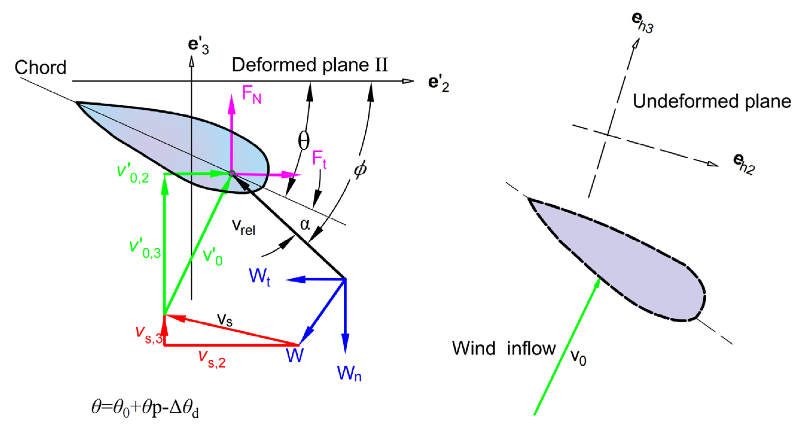
2.4. GE-BEM Aerodynamic Model

Under normal turbulent conditions, the blade tip deforms differently in different directions. The deformations are magnified in Figure 3, which illustrates the deformations in both the flapwise and edgewise directions, to provide a more intuitive understanding. Due to large deformations, the wind turbine rotor is no longer a flat plane but can be considered to possess a symmetric, bowl-shaped surface. Under these conditions, the flat-plane assumption is no longer reasonable. A very short segment at a distance s from the root of the blade, which is denoted as δs, was taken as the object of interest. Its sweeping motion forms the II trajectory, where II is a plane within which the momentum theorem can be adopted.
In order to apply the BEM method, a deformed rotor plane frame, e j o ; e 1 , e 2 , e 3 , was established at plane II. It was specified that o be located at the centroid of the deformed blade, while the e 1 direction is along the centroidal line of the blade, e 3 is normal to plane II and aligned with the incoming wind direction, and e 2 is tangent to plane II and perpendicular to e 1 . It is important to note that, due to the beam shear deformation, e 1 no longer coincides with t1 of the motion frame.
Due to the flapwise deformation of the blade, the deformed rotor plane, plane II, deviates from the ideally formed rotor plane, which is formed by straight blade sweeping. This deviation angle is equivalent to the blade cone angle, β , which was corrected by introducing the flapwise rotation angle obtained from the structural model. Consequently, the pre-bend angle at this point on the deformed rotor plane was adjusted to β + Δ β . Within plane II, because of the edgewise vibrational deformation of the blade, the blade element also changes in the tangential direction. This change is equivalent to the sweep angle of the blade σ . The variable Δ σ was introduced as a correction for this effect; it changes the blade sweep angle to σ + Δ σ . The transformation between the deformed rotor frame and the hub frame can be expressed by Equation (16):
e hj = R deform T e j R deform = R ( [ 0 , Δ β + β , 0 , ] T ) R ( [ 0 , 0 , σ + Δ σ ] T ) .
Figure 3 shows that a coordinate transformation must be used to transform the horizontal incoming wind speed v0 into the deformed rotor frame. The transformation relationship is given by Equation (17):
v 0 = R deform T R azi T R yaw T R η T v 0 .
Only the second and third components of v 0 participate in the calculations in the deformed rotor plane, while the first component, which is in the radial direction of the blade, can be neglected. The vibration speed is obtained in the blade root frame, so it must be transformed into the deformed rotor plane frame according to Equation (18):
v vibration = R deform T R hr ( x ˙ 0 + Ω × d s - e ) .
In Equation (18), x ˙ 0 represents the blade vibration speed vector, while the second term represents the velocity induced by the torsional blade vibration. Additionally, d s - e denotes the position vector of the aerodynamic center of the blade relative to the torsional center and Ω represents the angular velocity of the torsional blade vibration. The position vector of the blade element, x 0 ( s , t ) , is given by the structural model. The location change in the blade element caused by the blade vibration at s is denoted as Δ r = x 0 ( s , t ) x 0 ( s , 0 ) (when neglecting the blade location correction, Δ r = 0 ;   x 0 ( s , t ) = x 0 ( s , 0 ) ). The position vector in the hub frame is expressed by x h = r h u b , 0 , 0 T + R β x 0 , where r hub is the hub radius. Utilizing the rotor rotation vector, ω, the relative velocity of the wind at s caused by the turbine blade rotation can be determined (in the hub coordinate system):
v r = ω × x h .
Subsequently, the relative velocity in Equation (19) can be transformed into the deformed rotor plane frame, as shown in Equation (20):
v r = R deform T v r .
The velocity of the blade element consists of the velocities of the large-scale rigid rotation of the blade about the main axis of the rotor and the vibration of the blade itself. In this paper, this velocity is referred to as the structurally synthesized motion velocity, v s . Since velocity is relative, this velocity can be regarded as that of the wind moving toward the blade. It can be expressed by Equation (21):
v s = ( v r + v vibration ) .
Figure 4 shows that in the deformed rotor plane frame, the second and third components of v s were considered, while the first component, which is in the radial direction, was neglected. Thus, the airflow velocity relative to the blade element was decomposed into normal and tangential components in the deformed rotor frame. The magnitudes of these components can be calculated using Equation (22):
v n = v 0 , 3 + v s , 3 v t = v 0 , 2 + v s , 2 .
The derivation of the BEM model used in this study followed that presented by [37]. The axial and tangential induced velocities from momentum theory are expressed as W n = a v n and W t = a v t , respectively, where a is the axial induction factor and a is the tangential induction factor. The inflow velocity at a blade element in the deformed rotor frame can be calculated by v rel = ( 1 a ) 2 v n 2 + ( 1 + a ) 2 v t 2 , while the inflow angle is expressed by Equation (23):
ϕ = arctan v n ( 1 a ) v t ( 1 + a ) .
The attack angle at the blade element is given in Equation (24):
α = ϕ θ 0 θ p + Δ θ .
where θ0 represents the section twist angle, θ p is the pitch angle, and Δ θ is the blade twist deformation angle. For the 10 MW RWT, the corresponding lift coefficient, C L , drag coefficient, C D , and moment coefficient, C M can be obtained from the tables presented by [38]. Then, the normal aerodynamic force, FN, the tangential force, FT, and the aerodynamic torque, Ma, at the blade element can be calculated using Equation (25):
F N = 1 2 ρ v rel 2 c ( C L c o s ϕ + C D s i n ϕ ) F T = 1 2 ρ v rel 2 c ( C L s i n ϕ C D c o s ϕ ) M a = 1 2 ρ v rel 2 c 2 C M ,
where ρ is the air density and c represents the chord length. The blade tip loss correction factor is provided in Equation (26):
F = 2 π arccos exp ( B ( 1 ( x h / R 0 ) ) 2 ( x h / R 0 ) sin ϕ ) ,
where B is the number of blades and R 0 is the rotor radius. During the iterative calculation procedure that is followed when applying the BEM method, updated axial and tangential induction factors can be computed using Equations (27) and (28), respectively:
a new = 1 + 4 F J e sin 2 ϕ s l C L cos ϕ + C D sin ϕ 1 H 1 ,
a new = 4 F sin ϕ cos ϕ s l C L sin ϕ C D cos ϕ 1 1 ,
where s l = B c / 2 π x h , which represents the local solidity of the rotor. A local effective rotor radius correction was introduced by the expression J e = dx / ds cos ( β + Δ β ) . H is a correction factor, and if a o l d > 0.3539 , where a o l d is the axial induction factor in the previous time step, then H = 4 a o l d ( 1 a o l d ) 0.6 + 0.61 a o l d + 0.79 a o l d 2 . Pitt and Peter’s dynamic wake model [39] was adopted when accounting for unsteady aerodynamic effects, and the updated axial induction factor can be computed using Equation (29):
a new = ( v n C N B c Δ t + 8 π x h v n F sin 2 ϕ Δ t ) a old 2 ( v n C N B c Δ t + 16 F a old x h 2 sin 2 ϕ ) 2 a old ( v n C N B c Δ t + 8 π x h v n F sin 2 ϕ Δ t ) ( 2 v n C N B c Δ t + 8 π x h v n F sin 2 ϕ Δ t + 16 F x h 2 sin 2 ϕ ) ,
where Δ t is the simulation time step, C N = C L cos ϕ + C D sin ϕ , which is the normal aerodynamic force coefficient, and a ˙ represents the time derivative of the axial induction factor. After iterative convergence is achieved for a   and   a , the normal and tangential forces obtained must be transformed back into the root frame using the expression in Equation (30):
[ p r , p t , p n ] T = R ( [ 0 , Δ β , 0 ] T ) R ( [ 0 , 0 , Δ σ ] T ) [ 0 , F T , F N ] T .

2.5. Gravitational and Centrifugal Force Load Calculations

The gravitational force is defined in the global frame and is transformed to the root frame through an orthogonal transformation matrix, F g = R β R azi R η R yaw [ 0 ; 0 ; u ( s ) g ] T where g represents the gravitational acceleration. The centrifugal force can be more conveniently calculated in the hub frame, E hj , then transformed to the root frame through an orthogonal transformation matrix, F c = R β T x h ω 2 . This expression reflects the centrifugal stiffening effect, which causes larger deformations to produce greater centrifugal force components in the corresponding directions.
Because the shear center, elastic center, center of mass, and aerodynamic blade center do not coincide, the distribution of torque on the blade is quite complex. All the torques on the beam that were considered during this study are equivalent to the shear center of the blade; thus, the torques caused by the gravitational and centrifugal forces, which both act on the center of mass, can be expressed with respect to the blade shear center:
M g = d g × F g M c = d g × F c .
In Equation (31), d g represents the position vector from the shear center to the center of mass in the root frame.

2.6. Coupling Method

In time domain wind turbine simulations, prevalent coupling methods include both strong and weak coupling, which are also referred to as tight and loose coupling, respectively. Tight coupling demands strict adherence to conservation conditions between the fluid and structural domains, which necessitates continuous iteration and results in significant increases in computational costs. Research findings have indicated that the effects of using loose coupling rather than tight coupling for aeroelastic simulations are minimal and that loose coupling can meet computational cost requirements [22]. Notably, Sayed et al. (2019) [18], Sabale and Gopal (2019) [24], and Panteli et al. (2022) [25] all employed the loose coupling method. During this study, a loose coupling approach was adopted for the aeroelastic simulations, in which the structural response calculated during the preceding time step (which consists of the blade vibration velocity, the blade deformation, and the position) serves as the input for the load calculations performed in the subsequent time step. The external loads for the current step are computed using parameters from the previous step, which are assumed to remain constant during the structural dynamic response calculation iterations within the current time step. Figure 5 provides a flowchart of the aeroelastic coupling algorithm, in which the GEB model is utilized to calculate the blade structural response. When the Euler beam model is selected for calculation of the structural response, only the green portion of the flowchart must be replaced with a generic Euler beam solver.

3. Numerical Results

The GEB model that was established during this study was first verified using the static and dynamic portions of a benchmark case with a 45° pre-curved cantilever beam. This was performed to substantiate the analytical capability of the established GEB model to capture structural nonlinearity. A comparative assessment was also performed with the Euler beam model to explore the distinctions between linear and nonlinear models. Alongside the structural model, the aerodynamic model and the coupling method both affect the aeroelastic simulations significantly. Subsequently, a comparison was conducted with two globally acknowledged wind turbine simulation software packages, hGAST and DNV Bladed, to assess the dependability of the proposed aeroelastic model. Because these two software packages do not have open-source code and their core algorithms are proprietary, third parties cannot make corrections to them. Therefore, they were chosen to generate baseline results that were used to validate the model developed during this study. The geometry and material data, as well as the aerodynamic and control properties, were obtained from the DTU 10 MW RWT report [38]. The aeroelastic simulation model developed during this study was utilized, and an aerodynamic model without any corrections served as a baseline. A comparative analysis was performed to assess the effects of blade deformation on the aerodynamic loads and root loads of the wind turbine blade. Ultimately, a comparison was drawn between the simulation results of the aeroelastic model based on the GEB method and the Euler beam model results. Lastly, spectral and fatigue analyses were conducted to explore the impacts of structural nonlinearity on the blade loads.

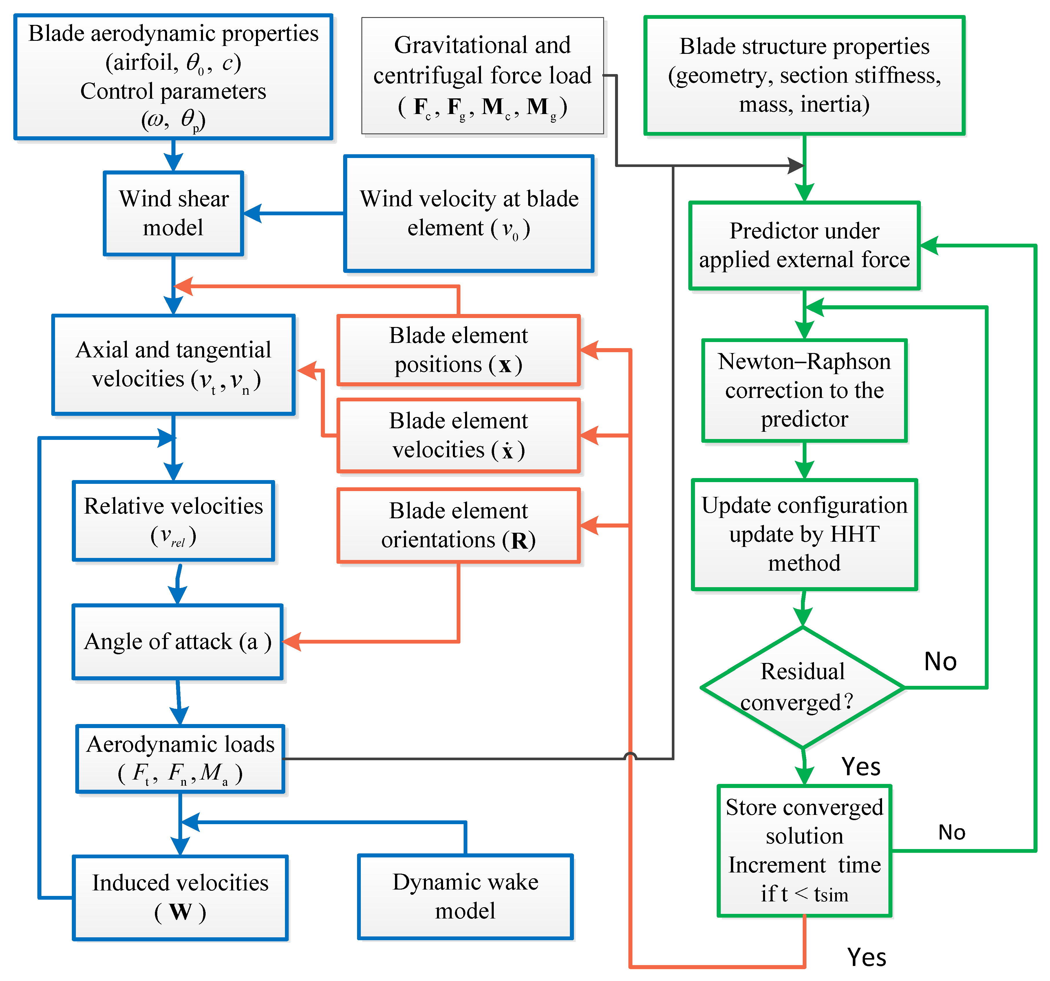
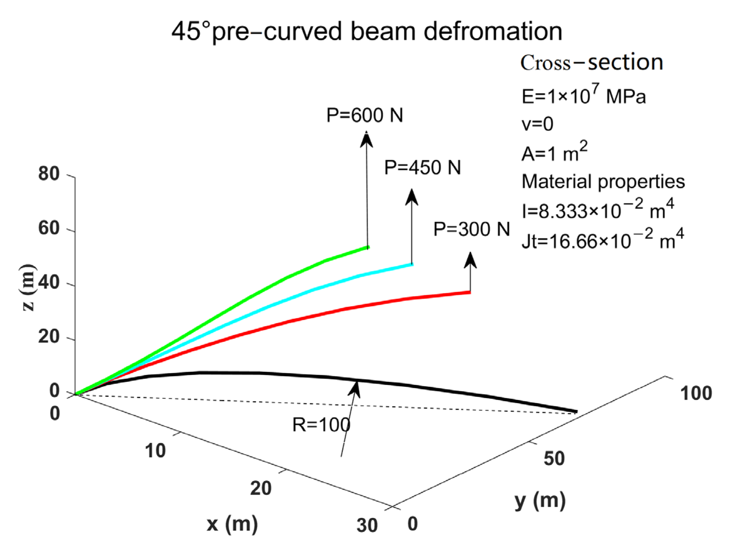
3.1. Benchmark Static Analysis with the 45° Pre-Curved Beam

A 45° pre-curved beam, which is characterized by substantial deformations and torsional nonlinearity, is frequently utilized as a benchmark to validate nonlinear structural models. Various wind turbine simulation tools have also employed this type of beam for computational validations [25,40]. To validate the GEB model developed during this study, the model was used to calculate the deformation of a 45° pre-curved beam when a steady load was applied on the free end of the beam. The geometric and material characteristics of the beam are provided in Figure 6, and the beam was discretized into eight beam elements. Steady loads of 300 N, 450 N, and 600 N were individually applied at the free end of the beam in the positive z-direction. A comparison of the position of the free end of the beam with other published results [31,34] is presented in Table 1. The results are highly consistent and therefore confirm the accuracy and reliability of the structural model developed during this study, which utilized the same internal force derivation method for the beam elements as did Cardona and Geradin (1988) [33]. Additionally, an analysis of the results revealed that, due to geometric nonlinearity, rotations around the x- and z-axes occur at the end of the beam along with rotation around the y-axis. The rotation vectors for the cross-section are presented in the fourth column of Table 1. In contrast, the linear Euler beam model could only calculate the rotation around the y-axis and was unable to capture the geometric nonlinearity.

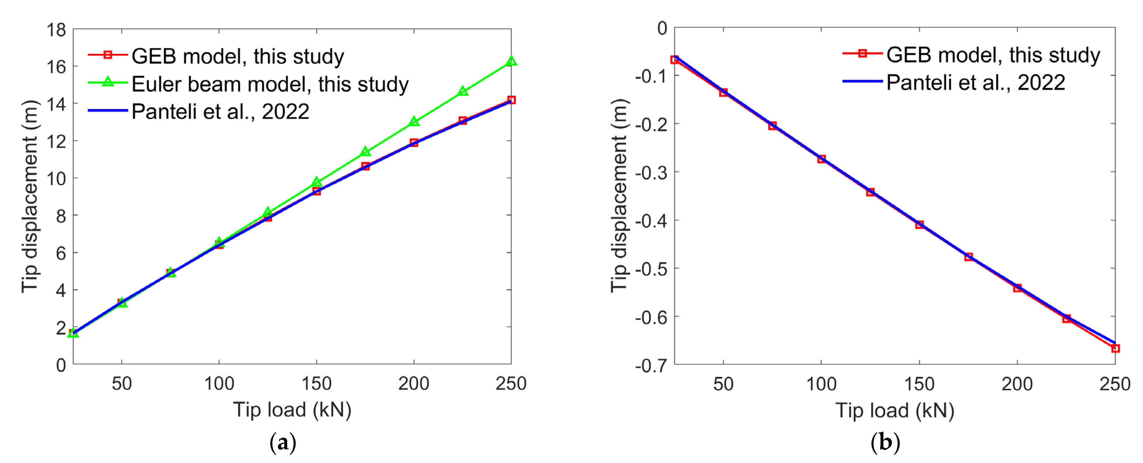
3.2. Static Deformation Analysis of the 10 MW RWT

To validate the analytical capability of the model developed during this study for beams with varying cross-sections and to explore the impact of geometric nonlinearity on actual blade deformations, deformation calculations were performed for the 10 MW RWT under static tip loading. Doing so involved utilizing both the GEB model and a linear Euler beam model. The blade used in this study was pre-bent by 3.3 m in the flapwise direction at the blade tip according to reference [38] and had no sweep. The blade was discretely divided into 50 beam elements, and material and geometric coupling was considered in both the flapwise and twist directions. Steady loads ranging from 25 to 250 kN were applied in the flapwise (e3) direction at the blade tip with a load increment of 25 kN.
The results, which are presented in Figure 7, demonstrate a strong agreement between the GEB model established during this study and hGAST software [25], which confirms the reliability and accuracy of the GEB model when it is used to analyze nonlinear beams with varying cross-sections. Figure 7a shows that the flapwise deformation is minimal when a small static load is applied at the blade tip and that Euler beam model results align with the GEB model results. As the load increases, significant deviations arise between the Euler beam and GEB model results. This deviation reaches 16% for a 250 kN blade tip load, thereby revealing the inability of the Euler beam model, which is based on the assumption of small linear deformations, to accurately represent the substantial blade deformations that exist in this scenario. Due to the aerodynamic twist and irregular cross-sections within the blades, bend–bend coupling motion arises in the flapwise and edgewise directions. The non-coincidence of the aerodynamic center, centroid, and shear center of the blade cross-section introduces a bending–torsion coupling effect, which results in blade deformations that are characterized by a coupled flexural and torsional response due to external loads. Figure 7b demonstrates that because of the existence of bend–bend coupling, displacement also occurs in the edgewise direction. Figure 7c shows that for a 250 kN static load, substantial torsional rotation occurs at the blade tip because of bend–twist coupling; this rotation reaches a maximum of 2.1°. Simultaneous displacement in the flapwise direction and negative displacement in the longitudinal direction cause the blade to shorten, as illustrated in Figure 7d. The linear Euler beam model, which is constrained by theoretical limits and the small deformation assumption, failed to capture the bend–bend and bend–twist coupling effects, and its small deformation assumption precluded the simulation of longitudinal displacement; thus, no Euler beam results could be included in Figure 7b–d.

3.3. Benchmark Dynamic Analysis with the 45° Pre-Curved Beam

Wind turbine blades, especially those with pre-bend and pre-twist characteristics, are typical slender nonlinear structures. Their structural dynamics closely resemble those of the benchmark 45° pre-curved cantilever beam. To validate the computational capability of the new GEB model when applied to nonlinear dynamic analyses, dynamic simulations were performed for the benchmark beam when it was subjected to external impulse loads. The simulation conditions are depicted in Figure 8a, which incorporates detailed geometric and material properties from the literature [41]. A comparison with the literature [41], which is presented in Figure 8b, substantiated the highly consistent and reliable dynamic computational capability of the model.

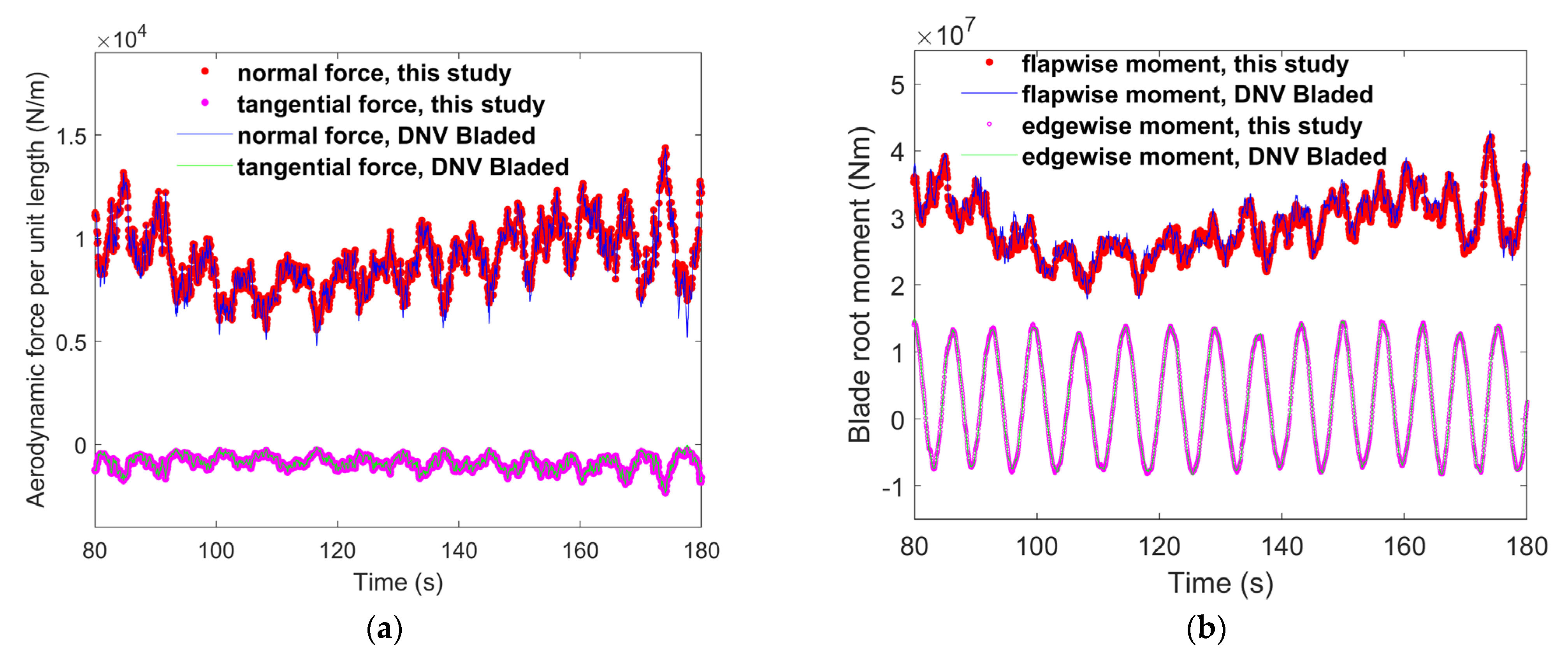
3.4. Load Calculations for the 10 MW RWT

To validate the aerodynamic and load calculation models established during this study, simulations were conducted for the 10 MW RWT using the proposed model. The simulation results were then compared with those obtained from DNV Bladed software [42] (version 4.3, which uses Timoshenko beam elements for structural modeling and the BEM method for aerodynamic modeling). This is a widely recognized wind turbine simulation software endorsed by many international wind turbine certification authorities. The simulations, which included no corrections to the BEM model, neglected the blade vibration effects on the inflow wind speed, thereby essentially treating the blade as rigid. A three-dimensional turbulent wind field with an average wind speed of 11.4 m/s and a turbulence intensity of 20%, which considered wind shear and a ground roughness coefficient, z 0 , of 0.2, was generated by DNV Bladed. Yaw misalignment and wind turbine faults were not considered. Initially, aerodynamic loads per unit length, p n and p t , were extracted for comparison at 0.8 R 0 from the rotor center, which is the primary power-producing region of the wind turbine blade. The results were compared over a 100 s interval, as shown in Figure 9a, for clarity. The comparison revealed excellent agreement between the aerodynamic load calculation results obtained during this study and those generated by DNV Bladed. Minor discrepancies were observed, and these were attributed to differences between the correction methods for large axial induction factors, a, applied in this study and DNV Bladed [42]. To further validate the capability of the aeroelastic model to compute the overall blade loads, flapwise and edgewise root moments obtained from the model for the same simulation conditions were compared with those from DNV Bladed. The comparison, which is illustrated in Figure 9b, demonstrates strong consistency between the results from this model and those from DNV Bladed. Minimal differences can be observed in the edgewise direction, and any slight variations in the flapwise direction were primarily attributed to differences between the correction methods for large axial induction factors in the BEM model.

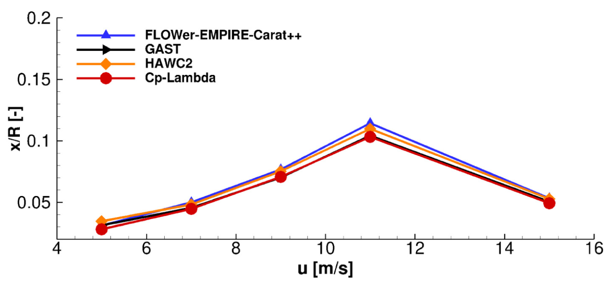
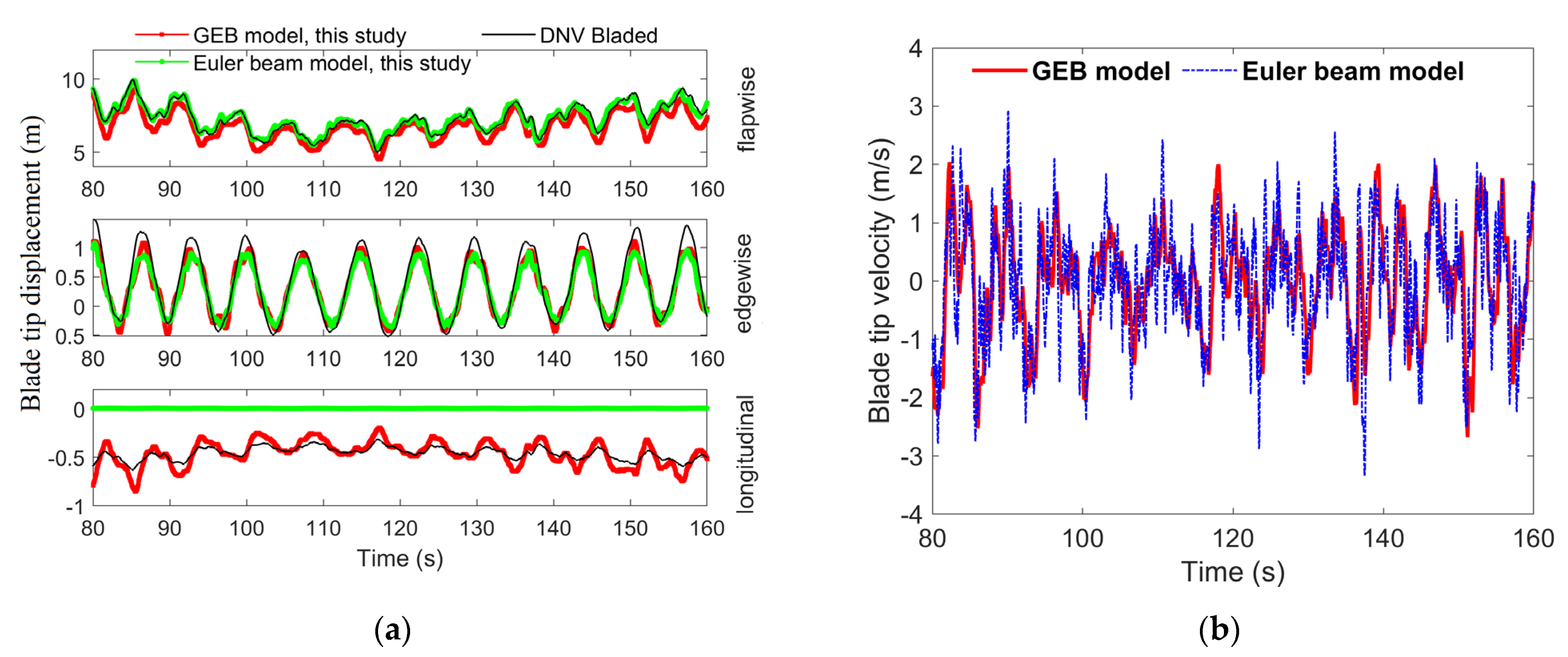
3.5. Aeroelastic Simulations of the 10 MW RWT

To validate the aeroelastic coupling model proposed in this paper and to investigate the impacts of structural nonlinearity on the dynamic response of the blade, the Euler beam and GEB models were independently integrated into the GE-BEM model, thereby forming an aeroelastic model. Simulations were conducted for the 10 MW RWT wind turbine under the 3D turbulent wind conditions outlined in Section 3.4. These simulations accounted for aeroelastic coupling while excluding deformation corrections to the BEM model, and the blade was discretely divided into 50 beam elements. The simulation results were compared with results obtained from DNV Bladed. For clarity, the blade tip displacement and velocity were isolated within an 80 s interval; the results are depicted in Figure 10.
Figure 10a shows that both aeroelastic coupling models established during this study, which were based on the GEB and Euler beam models, produced flapwise and edgewise blade tip displacements that closely aligned with those obtained from DNV Bladed. The tip displacements calculated using the Euler beam model were more similar to those predicted by DNV Bladed than to those obtained from the GEB model. This result primarily occurred because the structural model employed by DNV Bladed is the linear Timoshenko beam model. The linear Euler beam model produced blade tip displacements that were different from those obtained by the GEB model in the flapwise direction, which was characterized by significant deformation. This overestimation of flapwise deformation is consistent with the static analysis results presented in Section 3.2. In the edgewise direction, which exhibits only minor deformation, the blade tip displacement disparities are negligible. Furthermore, due to the small deformation assumption made by the Euler beam model, the longitudinal displacement calculated by the Euler beam model significantly deviated from those produced by the GEB model and DNV Bladed. The GEB model demonstrated more pronounced longitudinal displacement variations than DNV Bladed. According to momentum theory, the flapwise vibration velocity most significantly impacts the wind speed and, consequently, the wind turbine load; thus, the flapwise vibration velocities calculated by the GEB and Euler beam models were specifically compared, as shown in Figure 10b. It is apparent that the flapwise vibration velocity of the Euler beam model surpassed that of the GEB model. This result suggests that the linear beam model also overestimates the flapwise vibration velocity. This overestimation intensifies the feedback effect of the Euler beam model in the aeroelastic coupling model, thereby resulting in a decrease in the inflow velocity for the aerodynamic model and subsequent reductions in the aerodynamic loads. This phenomenon was further verified in a subsequent analysis.

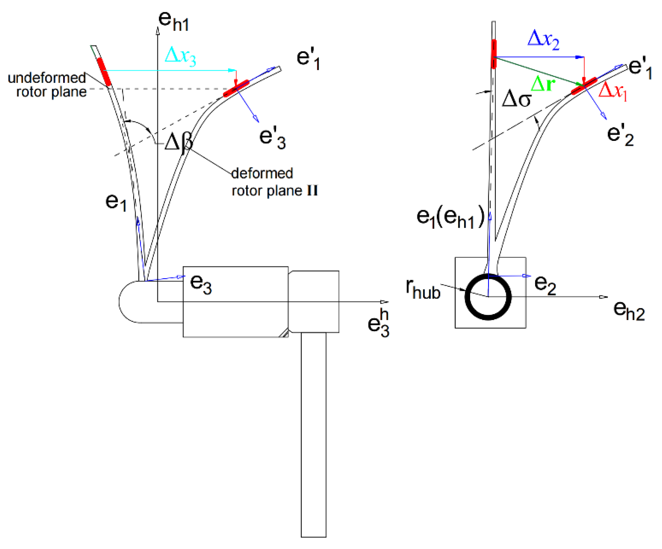
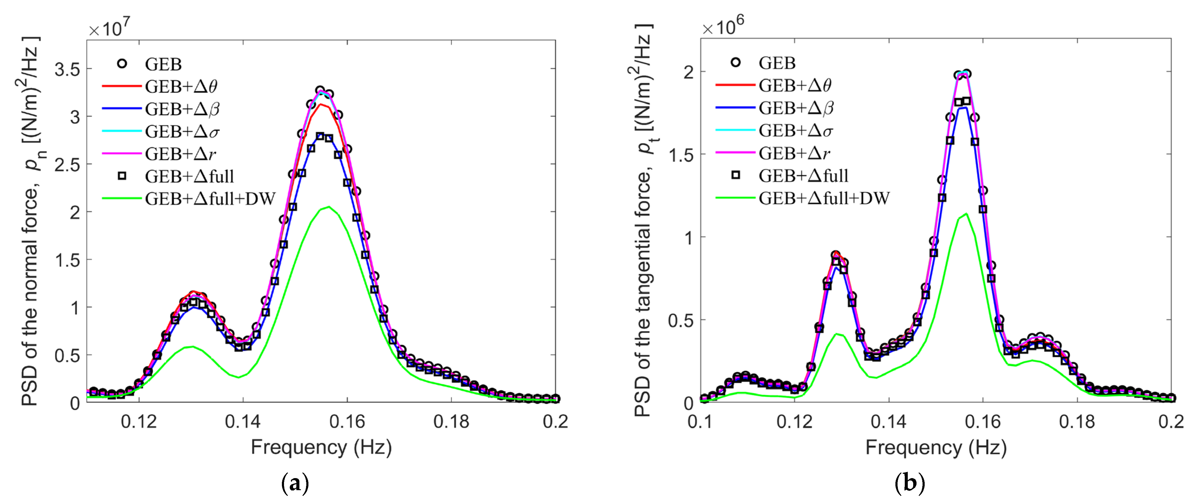
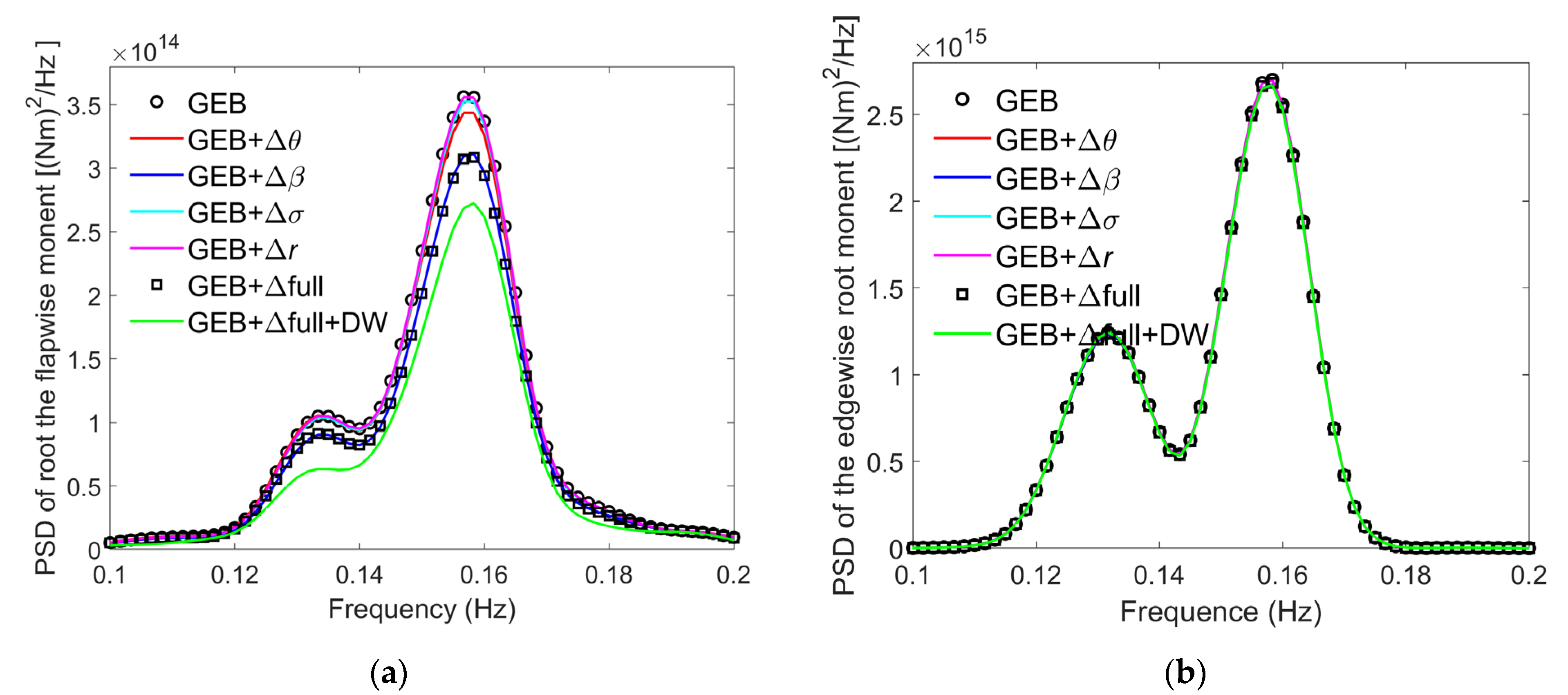
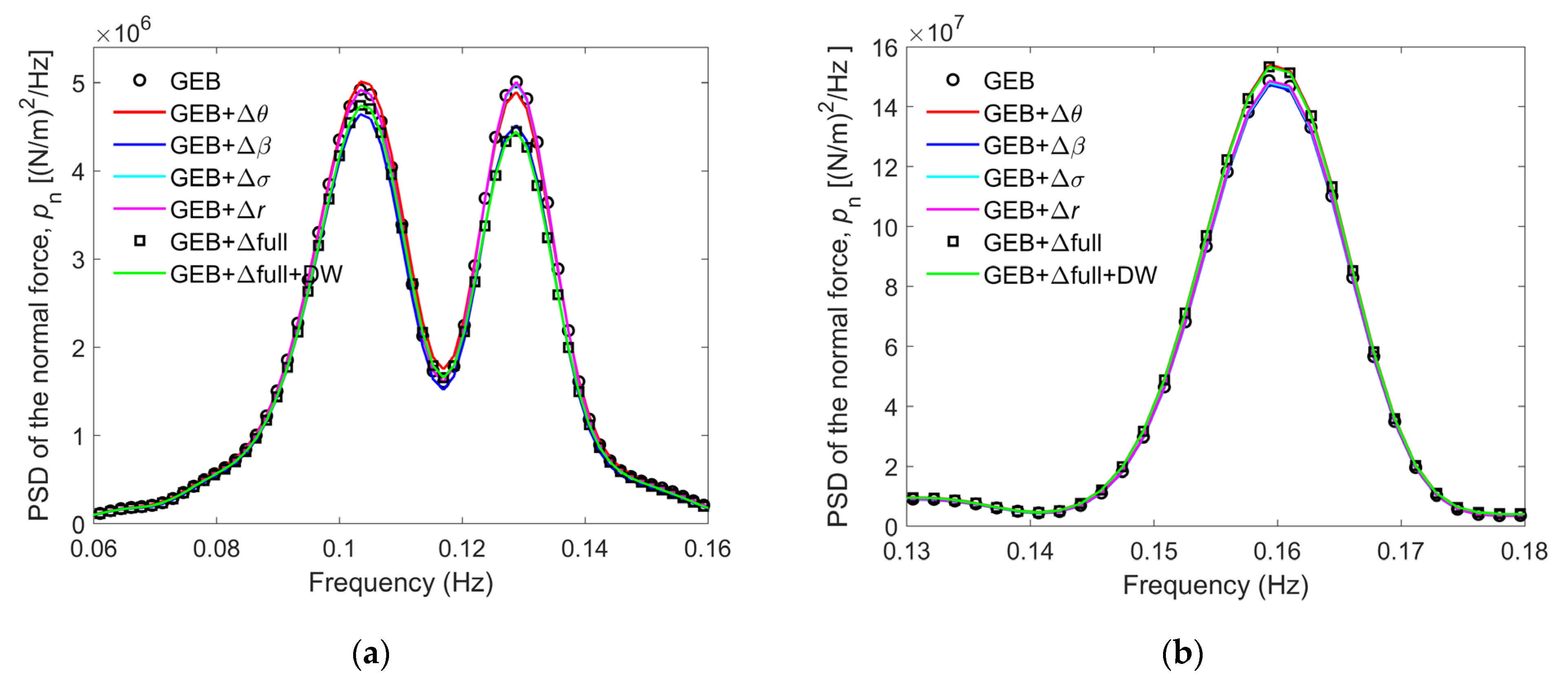
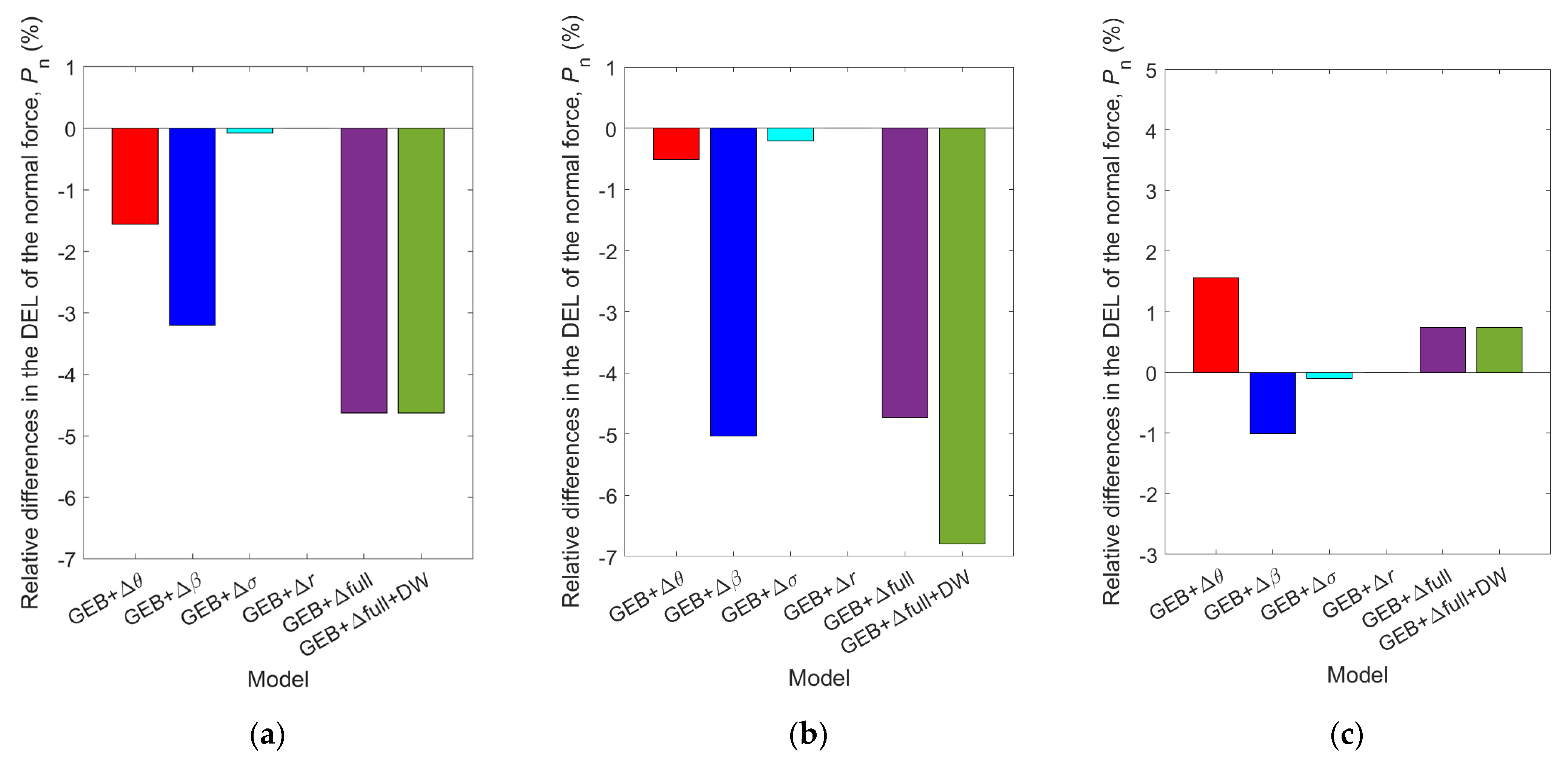
3.6. Influence of Deformation on the Blade Loads

To investigate the effects of deformation caused by vibration on the blade aerodynamic loads and the root loads, seven different aeroelastic models were established by introducing various corrections to the GE-BEM model that was previously validated. The corrections made in each model are described in the following list:
1.
A model was established with no deformation corrections or dynamic wake effects; it is referred to as GEB.
2.
A model was established with only a torsional deformation correction, Δ θ ; it is referred to as GEB + Δ θ .
3.
Another model, referred to GEB + Δ β , included only a flapwise deformation correction, Δ β .
4.
Only an edgewise deformation correction, Δ σ , was included in the fourth model, which is referred to as GEB + Δ σ .
5.
A model was established with a blade element location change correction, Δr; this model is referred to as GEB + Δr.
6.
A sixth model, referred to as GEB + Δ full , was established; it included all four corrections mentioned previously.
7.
The last model included all four corrections and a dynamic wake model; this model is referred to as GEB + Δfull + DW.
Utilizing the correction scheme described in this list, seven aeroelastic models using the Euler beam model were also established and named; they are denoted as Eu, Eu + Δ θ , Eu + Δ β , Eu + Δ σ , Eu + Δ full , and Eu + Δ full + DW , where Eu is an abbreviation for Euler.
Utilizing the seven aeroelastic models based on the GEB model, simulations were conducted for the 10 MW RWT for 600 s under turbulent wind conditions. The simulations used average wind speeds of 7 m/s, 11.4 m/s, and 24 m/s, which represent typical low, rated, and high wind speed operating conditions, respectively. Using all three wind speeds allowed for a comprehensive investigation of the effects of vibration-induced blade deformations on the aerodynamic loads at different wind speeds.
To examine the effects of blade deformation on the aerodynamic loads, the effects of the deformations on the input parameters for the aerodynamic calculations were first investigated. As inferred from the previous analysis, the flapwise deformations were substantial. First, the effects of the flapwise rotation deformation correction, Δβ, on the axial inflow velocity, vn, at the blade element were explored. For clarity and a distinct comparison, the results were extracted at 0.99 R 0 for 50 s under turbulent wind conditions with an average wind speed of 11.4 m/s, as illustrated in Figure 11a. It is apparent that incorporating the Δβ correction results in a decrease in vn, although the reduction is not significant. According to momentum theory, normal aerodynamic loads are proportional to the square of vn, and as a result, a decrease in vn implies significant load reductions. As depicted in Figure 11b, including the Δ θ correction produces a distinct decrease in the attack angle of the blade element at 0.99 R 0 . Based on these two analyses, it can be tentatively concluded that blade deformations contribute to passive reductions in aerodynamic loads.
To obtain a better understanding of the variations in blade loads, spectral analyses were conducted for the loads of the 10 MW RWT computed using the seven models discussed previously. They were conducted for 600 s under turbulent wind conditions with an average wind speed of 11.4 m/s. Figure 12 presents the power spectral densities (PSDs) of the aerodynamic loads at 0.8 R 0 , while Figure 13 depicts the PSDs of the root bending moments. Clearly, both the normal and tangential aerodynamic force PSDs have dominant peaks at a rotational frequency of 0.16 Hz (1P). These peaks are primarily caused by the turbulence rotational sampling of the blade as it rotates and repeatedly passes through turbulent eddies. It is evident from Figure 12 that the dynamic wake effect most significantly impacts the aerodynamic loads when the mean wind speed is 11.4 m/s. This effect substantially reduces the PSDs of the aerodynamic loads, p t and p n , because the dynamic wake model acts as a dynamic filter for the axial induction factor, thereby preventing it from changing rigidly. There is therefore a gradual change in the induced velocity, which prevents sharp fluctuations in the aerodynamic loads, thereby reducing the overall load. With respect to blade deformation, the flapwise rotation angle, Δ β , has the most significant impact on the aerodynamic loads in both the flapwise and edgewise directions. The torsional deformation angle, Δ θ , has the second-largest effect, while the edgewise deformation, Δ σ , and the blade element location change, Δ r , have minimal effects that are nearly negligible. All the deformation factors contribute to reductions in the blade aerodynamic loads.
Figure 13 presents comparisons of the PSDs of the root moments calculated by the seven models for a mean wind speed of 11.4 m/s. As for the aerodynamic loads, the dynamic wake effect significantly reduces the flapwise loads at the blade root. However, its impacts on the edgewise root loads are relatively minor, as shown in Figure 13b. With respect to the effects of the different deformations on the root loads, the flapwise rotation deformation exerts the most significant influence, followed by the torsional deformation. The other deformations only minimally affect the flapwise root loads, as shown in Figure 13a. All the deformation corrections exhibit minor impacts on the edgewise root moment because the flapwise loads primarily result from the aerodynamic forces, while the edgewise loads are primarily influenced by the gravitational forces.
To compare the blade deformation effects at different wind speeds, spectral analyses were conducted for the aerodynamic loads at 0.8 R 0 under turbulent wind conditions with average wind speeds of 7 m/s and 24 m/s, as shown in Figure 14. Comparisons of the PSDs of the normal aerodynamic force, p n , at R 0 (as depicted in Figure 11a and Figure 13a,b) reveal that Δ β has the most significant impact on the blade aerodynamic loads at low wind speeds, while Δ θ has the greatest influence at high wind speeds. This result is primarily caused by the torsional vibration of the blade, which gradually increases with the wind speed due to the geometric coupling effect. In contrast, the flapwise deformation of the blade reaches its maximum value at the rated wind speed and then decreases as the wind speed increases. The impact of the blade torsional deformation on the aerodynamic loads also gradually intensifies as the wind speed increases. The torsional deformation weakens the loads at low wind speeds, while at high wind speeds, it enhances them. The primary reasons for this phenomenon are presented next. When the radius exceeds 41.72 m, the FFA-W3-241 airfoil is used for the blade. The aerodynamic data for this airfoil are presented in Figure 15a. Figure 15b shows that, when the wind speed at the blade is 24 m/s, the FFA-W3-241 airfoil operates in the negative attack angle range. The introduction of the torsional deformation correction (which causes the blade to rotate toward the feathering direction) results in a negative twist deformation angle, Δ θ . According to Equation (24), a negative twist deformation angle leads to decreases in the attack angle, α. As α continues to grow in the negative direction, as shown in Figure 15a, Cl and Cd increase; additionally, according to Equation (25), the resultant force, FN, also increases. Since the blade elements in this location represent the primary power-production region of the blade, the blade flapwise loads ultimately increase as well. This situation is exactly opposite to that when the blade operates at low wind speeds. For low wind speeds, the attack angle of the main part of the blade is positive; thus, the torsional deformation correction reduces the attack angle, which consequently reduces the resultant aerodynamic force and, therefore, reduces the loads.
To further validate these deductions, damage equivalent load (DEL) analyses were conducted for the aerodynamic loads calculated by the different simulation models under turbulent wind conditions. DELs were used to represent the fatigue damage data contributed by each load. Specifically, the fatigue damage data for each load obtained by rain flow counting was converted into equivalent fatigue damage caused by a single load range repeated at a single frequency. According to the Miner’s rule [43], the DEL can be expressed by Equation (32):
D E L = 1 . . n s i m i T l i f e , i T s i m , i 1 . . n k k 1 N r e f N i , k ( S i , k A / ( 1 S i , k M / S b ) ) m 1 / m ,
where Nref = 1.0 × 10⁷, which corresponds to a 20-year lifetime damage count, and Ni,k represents the number of cycles at a certain load range, S i , k M , and a certain mean load, S i , k M , determined by rainflow counting. Tlife,i represents the period during which the turbine will operate at the given wind speed of the simulation time series number, i, T sim , i is the simulation time, and m is the slope of the SN curve, for which a value of 10 is typically chosen for glass-reinforced plastic (GRP) [44]. The mean value of the aerodynamic load in the normal direction exceeds its vibration amplitude, as shown in Figure 9a. The impact of the mean stress on the fatigue should not be overlooked; therefore, the Goodman correction for the mean stress effects on the fatigue was introduced [45], where S b represents the correction at the ultimate load of the blade (which corresponds to the load applied when the blade reaches its ultimate stress).
Fatigue analyses were conducted for the 600 s simulation effective results of the normal load, p n , at 0.8 R 0 generated by the seven simulation models with average wind speeds of 7 m/s, 11.4 m/s, and 24 m/s. To facilitate the comparison, the results from the GE model were used as a baseline. The relative differences in the DEL values of the baseline results and those calculated by the other six models are presented in Figure 16. It is evident from Figure 16 that the flapwise rotation and torsional angle corrections most significantly influence the aerodynamic fatigue loads, while the edgewise rotation angle and the blade element location change have relatively minor impacts. The dynamic wake correction has a smaller impact on the blade fatigue loads when the deformations are minimal, but it becomes more pronounced as the deformations increase. Blade deformations result in decreases in the fatigue loads at low wind speeds but increases at high wind speeds; these results provide further validation for the conclusions presented previously in this section.

3.7. Structural Nonlinearity Effects on the Aeroelastic Loads

It is evident from the analysis presented in Section 3.5 that the linear Euler beam model overestimates the blade deformations and vibration velocity. The further analyses discussed in Section 3.6 revealed that the flapwise and torsional blade deformations, along with the dynamic wake, significantly impact the blade aerodynamic loads. The factors that affect the blade aeroelastic loads are diverse, thereby rendering the situation complex. This section presents an analysis of the influence of structural nonlinearity on blade loads by contrasting the simulation results for the Euler beam model with those for the GEB model. To enhance the computational efficiency, six models were selectively employed as follows: the Eu, (Eu + Δfull), (Eu + Δfull + DW), GEB, (GEB + Δfull), and (GEB + Δfull + DW) models. Previous analyses indicated that blade deformation most significantly affects the flapwise loads. Therefore, the DELs of the normal aerodynamic loads, p n , at 0.8 R 0 and the PSDs of the flapwise root moments calculated by the six models for the 10 MW RWT blade under turbulent wind conditions with a mean wind speed of 11.4 m/s for a duration of 600 s were initially compared, as depicted in Figure 17. Subsequently, the DELs of the tangential aerodynamic loads, p t , and the PSDs of the edgewise root moments calculated by the six models were also compared, and these results are presented in Figure 18.
Figure 17 shows that for turbulent wind conditions with an average wind speed of 11.4 m/s, the introduction of deformation corrections or the dynamic wake effect decreases both the aerodynamic loads and the root loads, regardless of whether the overall simulation model is based on the GEB model or the Euler beam model. Figure 17a demonstrates that the DELs of the normal aerodynamic force per unit length at 0.8 R 0 generated by the simulation models based on the Euler beam model were consistently smaller than those produced by the GEB method. The DEL result produced by the Euler beam model was nearest to the GEB result when no corrections were considered, while the difference was largest when all the corrections were included. Figure 17b shows that, regardless of which corrections were considered, the Euler beam model consistently yielded smaller flapwise root moments than the GEB model.
Figure 18a shows that the comparison between the p t values calculated using the Euler beam model and the GEB model is similar to that for the p n values. The results from the Euler beam model are consistently smaller than those from the GEB model. This trend is also evident in Figure 18b, although the differences between the edgewise root moments calculated by the Euler beam and GEB models are not as pronounced as those between the flapwise root moments. The smaller differences occurred primarily because of the smaller in-plane deformations, which resulted in decreased aeroelastic coupling effects on the aerodynamic loads. Additionally, since the tangential loads are primarily caused by gravitational effects, deformations have relatively minor effects.
To investigate the blade deformation and structural nonlinearity effects on the fatigue loads during the 20-year operational lifetime of a wind turbine, extensive simulations and fatigue analyses were conducted in accordance with the specification of the IEC 61400-1 standard [46] (IEC 61400-1, 2003), where the design load case (DLC) 1.2 is considered. The simulations were performed under turbulent wind conditions with 11 different mean wind speeds that ranged from 5 to 25 m/s at 2 m/s intervals, and the blade was discretely divided into 50 beam elements. For each mean wind speed, three random turbulence “wind seeds” were used, and each “wind seed” had a duration of 630 s. These conditions resulted in the simulation of 33 load cases for each wind simulation model, and each load case had an effective duration of 600 s. These simulations accounted for wind shear (with a shear exponent, z0, of 0.20), while yaw misalignment and tower shadow were omitted for the sake of simplicity. The wind turbine class selected was 1A, which is the category for higher turbulence characteristics. The wind speed distribution followed a Weibull distribution [38] with a mean annual wind speed of 11.4 m/s and a shape parameter of 2. Throughout the 20-year lifetime, the total number of load cases for each average speed wind speed was scaled according to Weibull hours.
The DELs of the flapwise, edgewise, and torsional blade root moments calculated by the six different models are depicted in Figure 19. For a clearer comparison, the simulation results obtained from the GEB model were used as a reference. The results from the other five models were compared with these reference results, and the relative deviations are presented in Table 2. Furthermore, the relative deviations between the Eu + Δfull + DW and GEB + Δfull + DW models are also presented in Table 2.
Figure 19 shows that, regardless of whether the simulations utilized the Euler beam model or the GEB model, the deformations reduced the loads. A detailed comparison of the results is shown in Table 2. Additionally, an analysis and discussion of the results were conducted from four primary perspectives as follows:
(1)
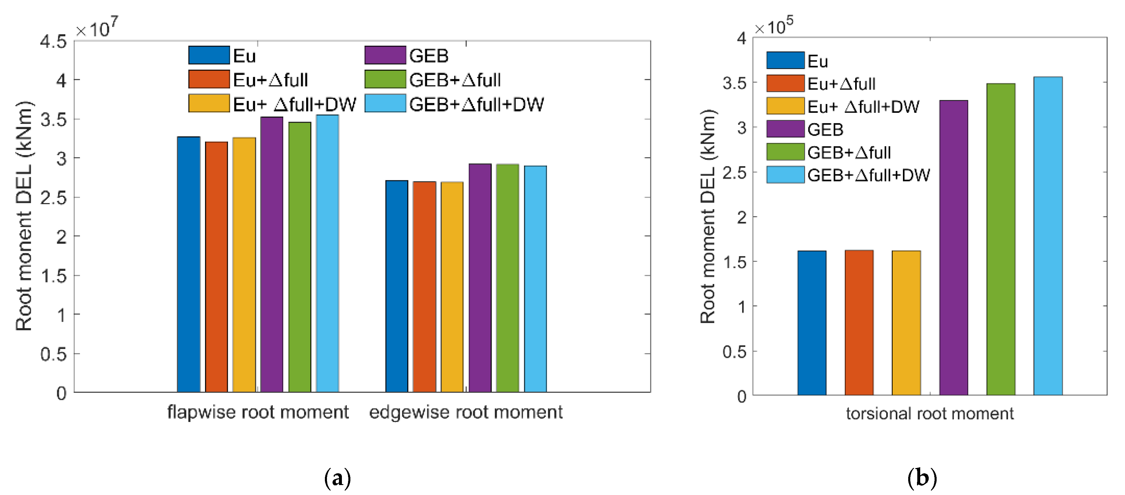
The differences between the results of the GEB + Δfull and GEB models can characterize the wind turbine blade deformation effects on the fatigue loads of the blade during its lifetime. The relative differences between the GEB + Δfull and GEB results in Table 2 show that the torsional root load is most affected by blade deformations, which caused a 5.73% increase in the DEL. Blade deformations have relatively smaller impacts on the flapwise root fatigue load, reducing the DEL by only 1.88%, while they have almost no effect on the edgewise root fatigue load.
(2)
The differences between the results generated by the GEB + Δfull + DW and GEB models reflect the dynamic wake effects on the blade fatigue loads. The relative differences between the results of these models presented in Table 2 indicate that the dynamic wake increases both the flapwise and torsional root fatigue loads but reduces the edgewise root fatigue load.
(3)
The differences between the Eu and GEB model results characterize the fatigue load differences solely by structural nonlinearity effects. The relative differences between the EU and GEB model results in Table 2 indicate that, throughout the lifetime of the wind turbine, the Euler beam model calculates fatigue loads that are smaller than those generated by the GEB model in all three directions. The largest difference was obtained for the DEL of the torsional root load; the value calculated by the Eu model was 51.97% less than that generated by the GEB model. The DELs of the flapwise and edgewise root bending moments obtained by the Euler beam model were 7.16% less than those calculated by the GEB model. These differences demonstrate that the linear structural model tends to underestimate fatigue loads.
(4)
The differences between the Eu + Δfull + DW and GEB + Δfull + DW models can characterize the variations in the fatigue loads that result from the combined wind turbine structural nonlinearity, blade deformation, and dynamic wake effects; accounting for these effects allows the simulations to align more closely with practical considerations. These relative differences are presented in the last column of Table 2, and they indicate that when accounting for the dynamic wake, the Euler beam model calculated a torsional fatigue load that was 54.49% less than that produced by the GE model, while the calculated flapwise and edgewise loads were 8.24% and 7.26% smaller, respectively. Furthermore, a comparison of the sixth and third columns reveals that including the dynamic wake effects amplifies the differences in the fatigue loads caused by the structural nonlinearity effects.

4. Conclusions

In this study, a blade structural analysis model was established using the geometrically exact beam (GEB) theory. It achieved an accurate representation of the significant deformations experienced by wind turbine blades. Subsequently, the blade element momentum (BEM) theory was corrected using the geometrically exact method to describe the wind velocity for a deformed blade, and a GE-BEM model was developed. Finally, an aeroelastic simulation model was established by coupling the structural and aerodynamic models. The validity of the developed model was confirmed by comparing its results for a pre-curved beam and a 10 MW RWT with those of commercial wind turbine simulation software packages. Simultaneously, the impacts of blade deformation on the aerodynamic performance were investigated using the GE-BEM model. Finally, a comparative analysis of aeroelastic simulation results obtained by the linear Euler–Bernoulli beam model (Euler beam model) and the GEB model was conducted to explore the influence of geometric nonlinearity on the blade aeroelastic loads. This study produced four primary conclusions:
(1)
A comparison with two commercial wind turbine simulation software packages demonstrated that the aeroelastic simulation model developed during this study is reliable. The GE-BEM model established during this study more accurately calculates the wind velocity at the blade elements, thereby bringing the simulation results closer to reality.
(2)
When a wind turbine operates near the rated wind speed, the flapwise deformation of the blades is at a maximum, and this deformation has the greatest impact on the aerodynamic loads. When a blade operates at high wind speeds, however (near the cut-out wind speed), the torsional vibration of the blade most significantly affects the aerodynamic loads.
(3)
Flapwise deformation of a turbine blade reduces the blade loads, while torsional deformation of the blade decreases the blade loads at low wind speeds but increases them at high wind speeds.
(4)
Due to the overestimation of both the blade deformation and the vibration speed by the Euler beam model, and consequently the overestimation of feedback to the aerodynamic model, the blade loads are underestimated by this model. The difference between DEL values calculated by the Euler beam model and the GEB model developed during this study was largest in the torsional root direction, with a maximum deviation of 53.5%.
As the enlargement of wind turbines has progressed, it has become evident that the linear Euler beam model is inadequate for the characterization of the associated intricate and large blade deformations. The analyses performed during this research emphasized that the structural nonlinearity of the blades causes increases in the fatigue loads, and traditional aeroelastic simulation models based on linear beam models underestimate the blade loads, especially in the torsional direction. This issue deserves careful consideration during the initial wind turbine design stage. In addition, when conducting aeroelastic simulations for wind turbines, the structural nonlinearity of the blades must be considered, and deformation corrections should be introduced into the traditional BEM model.

Author Contributions

Conceptualization, X.M. and J.S.; methodology, X.M. and X.P.; software, X.M. and Z.H.; validation, X.M., J.S. and Y.C.; formal analysis, X.M.; investigation, X.M. and X.P.; resources, X.M.; data curation, X.M. and Z.H.; writing—original draft preparation, X.M.; writing—review and editing, X.M.; visualization, X.M.; supervision, Y.C.; project administration, Y.C.; funding acquisition, Y.C. All authors have read and agreed to the published version of the manuscript.

Funding

This research was funded by [National Key Research and Development Program of China] grant number [2022YFB4201200] and National Natural Science Foundation of China projects grant number (No. 51976113).

Institutional Review Board Statement

Not applicable.

Informed Consent Statement

Not applicable.

Data Availability Statement

Data is contained within the article.

Acknowledgments

The authors would like to thank all the scientists, engineers, and students who participated in the wind energy researching field.

Conflicts of Interest

All the authors declare no conflicts of interest.

References

  1. Jahani, K.; Langlois, R.G.; Afagh, F.F. Structural Dynamics of Offshore Wind Turbines: A Review. Ocean Eng. 2022, 251, 111136. [Google Scholar] [CrossRef]
  2. Wind Energy in Europe: 2023 Statistics and the Outlook for 2024–2030. WindEurope. Available online: https://windeurope.org/intelligence-platform/product/wind-energy-in-europe-2023-statistics-and-the-outlook-for-2024-2030/#overview (accessed on 4 March 2024).
  3. World’s Largest Single Capacity Offshore Wind Turbine Successfully Installed—Global Times. Available online: https://www.globaltimes.cn/page/202306/1293347.shtml (accessed on 23 November 2023).
  4. World’s Largest 18 MW Offshore Wind Turbine Rolls off Assembly Line—CGTN. Available online: https://news.cgtn.com/news/2023-11-12/World-s-largest-18-MW-offshore-wind-turbine-rolls-off-assembly-line-1oFWaJ9ZQnm/index.html (accessed on 23 November 2023).
  5. Igwemezie, V.; Mehmanparast, A.; Kolios, A. Current Trend in Offshore Wind Energy Sector and Material Requirements for Fatigue Resistance Improvement in Large Wind Turbine Support Structures—A Review. Renew. Sustain. Energy Rev. 2019, 101, 181–196. [Google Scholar] [CrossRef]
  6. Soares-Ramos, E.P.P.; de Oliveira-Assis, L.; Sarrias-Mena, R.; Fernández-Ramírez, L.M. Current Status and Future Trends of Offshore Wind Power in Europe. Energy 2020, 202, 117787. [Google Scholar] [CrossRef]
  7. Manolas, D.I.; Riziotis, V.A.; Voutsinas, S.G. Assessing the Importance of Geometric Nonlinear Effects in the Prediction of Wind Turbine Blade Loads. J. Comput. Nonlinear Dyn. 2015, 10, 041008. [Google Scholar] [CrossRef]
  8. Griffith, D.T.; Ashwill, T.D. The Sandia 100-Meter All-Glass Baseline Wind Turbine Blade: SNL100-00; Sandia National Laboratories: Albuquerque, Mexico, 2011. [Google Scholar]
  9. Wang, L.; Liu, X.; Renevier, N.; Stables, M.; Hall, G.M. Nonlinear Aeroelastic Modelling for Wind Turbine Blades Based on Blade Element Momentum Theory and Geometrically Exact Beam Theory. Energy 2014, 76, 487–501. [Google Scholar] [CrossRef]
  10. Wang, X.; Cai, C.; Cai, S.-G.; Wang, T.; Wang, Z.; Song, J.; Rong, X.; Li, Q. A Review of Aerodynamic and Wake Characteristics of Floating Offshore Wind Turbines. Renew. Sustain. Energy Rev. 2023, 175, 113144. [Google Scholar] [CrossRef]
  11. Ahlström, A. Influence of Wind Turbine Flexibility on Loads and Power Production. Wind Energy 2006, 9, 237–249. [Google Scholar] [CrossRef]
  12. Liu, X.; Lu, C.; Liang, S.; Godbole, A.; Chen, Y. Vibration-Induced Aerodynamic Loads on Large Horizontal Axis Wind Turbine Blades. Appl. Energy 2017, 185, 1109–1119. [Google Scholar] [CrossRef]
  13. Wang, L.; Liu, X.; Kolios, A. State of the Art in the Aeroelasticity of Wind Turbine Blades: Aeroelastic Modelling. Renew. Sustain. Energy Rev. 2016, 64, 195–210. [Google Scholar] [CrossRef]
  14. Dai, J.; Li, M.; Chen, H.; He, T.; Zhang, F. Progress and Challenges on Blade Load Research of Large-Scale Wind Turbines. J. Dai 2022, 196, 482–496. [Google Scholar] [CrossRef]
  15. Zhong, W.; Shen, W.Z.; Wang, T.G.; Zhu, W.J. A New Method of Determination of the Angle of Attack on Rotating Wind Turbine Blades. Energies 2019, 12, 4012. [Google Scholar] [CrossRef]
  16. Sun, Z.; Chen, J.; Shen, W.Z.; Zhu, W.J. Improved Blade Element Momentum Theory for Wind Turbine Aerodynamic Computations. Renew. Energy 2016, 96, 824–831. [Google Scholar] [CrossRef]
  17. Fritz, E.K.; Ferreira, C.; Boorsma, K. An Efficient Blade Sweep Correction Model for Blade Element Momentum Theory. Wind Energy 2022, 25, 1977–1994. [Google Scholar] [CrossRef]
  18. Sayed, M.; Klein, L.; Lutz, T.; Krämer, E. The Impact of the Aerodynamic Model Fidelity on the Aeroelastic Response of a Multi-Megawatt Wind Turbine. Renew. Energy 2019, 140, 304–318. [Google Scholar] [CrossRef]
  19. Rezaei, M.M.; Behzad, M.; Haddadpour, H.; Moradi, H. Development of a Reduced Order Model for Nonlinear Analysis of the Wind Turbine Blade Dynamics. Renew. Energy 2015, 76, 264–282. [Google Scholar] [CrossRef]
  20. Zhang, P.; Huang, S. Review of Aeroelasticity for Wind Turbine: Current Status, Research Focus and Future Perspectives. Front. Energy 2011, 5, 419–434. [Google Scholar] [CrossRef]
  21. Rafiee, R.; Tahani, M.; Moradi, M. Simulation of Aeroelastic Behavior in a Composite Wind Turbine Blade. J. Wind Eng. Ind. Aerodyn. 2016, 151, 60–69. [Google Scholar] [CrossRef]
  22. Della Posta, G.; Leonardi, S.; Bernardini, M. A Two-Way Coupling Method for the Study of Aeroelastic Effects in Large Wind Turbines. Renew. Energy 2022, 190, 971–992. [Google Scholar] [CrossRef]
  23. Mo, W.; Li, D.; Wang, X.; Zhong, C. Aeroelastic Coupling Analysis of the Flexible Blade of a Wind Turbine. Energy 2015, 89, 1001–1009. [Google Scholar] [CrossRef]
  24. Sabale, A.; Gopal, K.V.N. Nonlinear Aeroelastic Response of Wind Turbines Using Simo-Vu-Quoc Rods. Appl. Math. Model. 2019, 65, 696–716. [Google Scholar] [CrossRef]
  25. Panteli, A.N.; Manolas, D.I.; Riziotis, V.A.; Spiliopoulos, K.V. Comparative Study of Two Geometrically Non-Linear Beam Approaches for the Coupled Wind Turbine System. J. Wind Eng. Ind. Aerodyn. 2022, 231, 105231. [Google Scholar] [CrossRef]
  26. Finnegan, W.; Jiang, Y.; Dumergue, N.; Davies, P.; Goggins, J. Investigation and Validation of Numerical Models for Composite Wind Turbine Blades. J. Mar. Sci. Eng. 2021, 9, 525. [Google Scholar] [CrossRef]
  27. Sayed, M.; Lutz, T.; Krämer, E.; Shayegan, S.; Wüchner, R. Aeroelastic Analysis of 10 MW Wind Turbine Using CFD–CSD Explicit FSI-Coupling Approach. J. Fluids Struct. 2019, 87, 354–377. [Google Scholar] [CrossRef]
  28. Fan, Q.; Wang, X.; Yuan, J.; Liu, X.; Hu, H.; Lin, P. A Review of the Development of Key Technologies for Offshore Wind Power in China. J. Mar. Sci. Eng. 2022, 10, 929. [Google Scholar] [CrossRef]
  29. Argyris, J. An Excursion into Large Rotations. Comput. Methods Appl. Mech. Eng. 1982, 32, 85–155. [Google Scholar] [CrossRef]
  30. Reissner, E. On One-Dimensional Finite-Strain Beam Theory: The Plane Problem. Z. Angew. Math. Phys. ZAMP 1972, 23, 795–804. [Google Scholar] [CrossRef]
  31. Simo, J.C.; Vu-Quoc, L. On the Dynamics of Flexible Beams Under Large Overall Motions—The Plane Case: Part II. J. Appl. Mech. 1986, 53, 855–863. [Google Scholar] [CrossRef]
  32. Simo, J.C. A Finite Strain Beam Formulation. The Three-Dimensional Dynamic Problem. Part I. Comput. Methods Appl. Mech. Eng. 1985, 49, 55–70. [Google Scholar] [CrossRef]
  33. Simo, J.C.; Vu-Quoc, L. A Three-Dimensional Finite-Strain Rod Model. Part II: Computational Aspects. Comput. Methods Appl. Mech. Eng. 1986, 58, 79–116. [Google Scholar] [CrossRef]
  34. Cardona, A.; Geradin, M. A Beam Finite Element Non-linear Theory with Finite Rotations. Numer. Meth Eng. 1988, 26, 2403–2438. [Google Scholar] [CrossRef]
  35. Hilber, H.M.; Hughes, T.J.R.; Taylor, R.L. Improved Numerical Dissipation for Time Integration Algorithms in Structural Dynamics. Earthq. Eng. Struct. Dyn. 1977, 5, 283–292. [Google Scholar] [CrossRef]
  36. Chung, J.; Hulbert, G. A Time Integration Algorithm for Structural Dynamics with Improved Numerical Dissipation: The Generalized-α Method. ASME J. Appl. Mech. 1993, 60, 371–375. [Google Scholar] [CrossRef]
  37. Hansen, M.O.L. Aerodynamics of Wind Turbines, 3rd ed.; Earthscan from Routledge: London, UK, 2015; ISBN 978-1-138-77507-7. [Google Scholar]
  38. Bak, C.; Zahle, F.; Bitsche, R.; Kim, T.; Yde, A.; Henriksen, L.C.; Hansen, M.H.; Blasques, J.P.A.A.; Gaunaa, M.; Natarajan, A. The DTU 10-MW Reference Wind Turbine. DTU Wind Energy Report-I-0092. In Danish Wind Power Research. 2013. Available online: https://backend.orbit.dtu.dk/ws/portalfiles/portal/55645274/The_DTU_10MW_Reference_Turbine_Christian_Bak.pdf (accessed on 19 March 2024).
  39. Pitt, D.M.; Peters, D.A. Theoretical Prediction of Dynamic-in Ow Derivatives; University of Bristol: Bristol, UK, 1981. [Google Scholar]
  40. Wang, Q.; Sprague, M.A.; Jonkman, J.; Johnson, N.; Jonkman, B. BeamDyn: A High-fidelity Wind Turbine Blade Solver in the FAST Modular Framework. Wind Energy 2017, 20, 1439–1462. [Google Scholar] [CrossRef]
  41. Le, T.-N.; Battini, J.-M.; Hjiaj, M. Dynamics of 3D Beam Elements in a Corotational Context: A Comparative Study of Established and New Formulations. Finite Elem. Anal. Des. 2012, 61, 97–111. [Google Scholar] [CrossRef]
  42. Bossanyi, E. GH Bladed Theory Manual; GH & Partners Ltd.: New Barnet, Hertfordshire, UK, 2003. [Google Scholar]
  43. Miner, M.A. Cumulative damage in fatigue. J. Appl. Mech. 1945, 67, A159–A164. [Google Scholar] [CrossRef]
  44. Lloyd, G.; Hamburg, G. Guideline for the Certification of Offshore Wind Turbines 2005; Germanischer Lloyd Wind Energie GmbH: Hamburg, Germany, 2005. [Google Scholar]
  45. Lee, Y.-L. (Ed.) Fatigue Testing and Analysis: Theory and Practice; Elsevier Butterworth-Heinemann: Amsterdam, The Netherlands; ISBN 978-0-7506-7719-6.
  46. IEC 61400-1; Wind Turbines—Part 1: Design Requirements (3rd ed.). International Electrotechnical Commission: London, UK, 2005.
Figure 1. Normalized flapwise deformation at the blade tip for different wind speeds [27].
Jmse 12 00548 g001
Figure 2. (a) Wind turbine coordinate systems [24]. (b) Initial and deformed configurations of the GEB.
Jmse 12 00548 g002
Figure 3. Schematic of the blade deformation and the deformed rotor plane frame.
Jmse 12 00548 g003
Figure 4. Airflow velocity vectors and aerodynamic forces in the deformed rotor frame.
Jmse 12 00548 g004
Figure 5. Flowchart of the aeroelastic module algorithm.
Jmse 12 00548 g005
Figure 6. Deformation diagram and calculation conditions for the 45° pre-curved beam.
Jmse 12 00548 g006
Figure 7. Tip displacement and rotation of the 10 MW RWT blade under flapwise static tip loading: (a) flapwise tip displacement, (b) edgewise tip displacement, (c) torsional tip rotation, and (d) longitudinal tip displacement compared with hGAST software [25].
Jmse 12 00548 g007aJmse 12 00548 g007b
Figure 8. (a) Loading and being of the 45° pre-curved cantilever beam [41] and (b) beam free end time–history responses compared with reference [41].
Jmse 12 00548 g008
Figure 9. (a) Aerodynamic loads at 0.8 R 0 for the 10 MW RWT and (b) blade root moments of the 10 MW RWT.
Jmse 12 00548 g009
Figure 10. (a) Blade tip response under turbulent wind conditions and (b) blade tip flapwise velocity.
Jmse 12 00548 g010
Figure 11. (a) Axial inflow wind speed at 0.99 R 0 in the time domain and (b) attack angle at 0.99 R 0 in the time domain.
Jmse 12 00548 g011
Figure 12. PSDs of the aerodynamic forces per unit length at 0.8 R 0 under turbulent wind conditions with an average wind speed of 11.4 m/s: (a) normal aerodynamic force PSD, p n , and (b) tangential aerodynamic force PSD, p t .
Jmse 12 00548 g012
Figure 13. PSDs of the root moments under turbulent wind conditions with an average wind speed of 11.4 m/s: (a) flapwise direction and (b) edgewise direction.
Jmse 12 00548 g013
Figure 14. PSDs of the aerodynamic forces per unit length, p n , at 0.8 R 0 under turbulent wind conditions with average wind speeds of (a) 7 m/s and (b) 24 m/s.
Jmse 12 00548 g014
Figure 15. (a) Data for the FFA-W3-241 airfoil. (b) Attack angle distribution of the blade.
Jmse 12 00548 g015
Figure 16. Relative differences in the DELs of the aerodynamic forces per unit length at 0.8 R 0 calculated by the six correction models and the baseline model under turbulent wind fields with mean wind speeds of (a) 7 m/s, (b) 11.4 m/s, and (c) 24 m/s.
Jmse 12 00548 g016
Figure 17. Results from six different simulation models for a turbulent wind field with a mean wind speed of 11.4 m/s: (a) DELs of the normal aerodynamic forces per unit length at 0.8 R 0 and (b) PSDs of the flapwise root bending moments.
Jmse 12 00548 g017
Figure 18. Results from six simulation models for a turbulent wind field with a mean wind speed of 11.4 m/s: (a) DELs of the tangential aerodynamic forces per unit length at 0.8 and (b) PSDs of the edgewise root bending moments.
Jmse 12 00548 g018
Figure 19. DELs of the blade root loads calculated by the six different models: (a) flapwise and edgewise root moments and (b) torsional root moments.
Jmse 12 00548 g019
Table 1. Position of the free end of the 45° pre-curved beam under free end loading.
LoadPosition Calculated during This Study,
(x1, x2, x3) (m)
Cardona and Geradin [34],
(x1, x2, x3) (m)
Simo and Vu-Quoc [31],
(x1, x2, x3) (m)
Rotation Vector, Ψ
300 N(22.26, 58.88, 40.08)(22.14, 58.64, 40.35)(22.33, 58.84, 40.08)(0.72, −0.49, 0.02)
450 N(18.40, 52.27, 48.40)(18.38, 52.11, 48.59)(18.62, 52.32, 48.39)(0.91, −0.50, 0.04)
600 N(15.67, 47.30, 53.37)(15.55, 47.04, 53.50)(15.79, 47.23, 53.37)(1.03, −0.55, 0.05)
Table 2. Comparison of the blade root moment DEL values of the six different models.
ModelGEBEUGEB + ΔfullGEB + Δfull + DWEu + Δfull + DW
Reference modelDEL (kNm)GEBGEBGEBGEB + Δfull + DW
Relative differencediff (%)diff (%)diff (%)diff (%)
Flapwise root moment35,192−7.16−1.880.88−8.24
Edgewise root moment29,166−7.19−0.14−0.61−7.26
Torsional root moment330−5.975.737.92−54.49
Disclaimer/Publisher’s Note: The statements, opinions and data contained in all publications are solely those of the individual author(s) and contributor(s) and not of MDPI and/or the editor(s). MDPI and/or the editor(s) disclaim responsibility for any injury to people or property resulting from any ideas, methods, instructions or products referred to in the content.

