Abstract
The presence of complex electromagnetic noise in the ocean significantly impacts the accuracy of ship shaft-rate electric field signal detection, necessitating the development of an effective denoising method to enhance detection precision. Nevertheless, traditional denoising methods encounter issues like low frequency resolution, challenging threshold configuration, and mode mixing. This study introduces a method that integrates variational mode decomposition (VMD) with multi-window spectral subtraction (MSS). The intrinsic mode functions (IMFs) of noisy signals are extracted using VMD, and the noise components within different IMFs are identified. The spectral features of both signal and noise within different IMFs are leveraged to eliminate noise signals via MSS. Subsequently, the denoised components of IMFs are rearranged to derive the denoised ship shaft-rate electric field signals, achieving noise reduction across various frequency bands. Following validation using simulation signals and empirical data, the noise reduction efficacy of VMD-MSS surpasses that of alternative methods, demonstrating robust performance even at low signal-to-noise ratios. The marine electromagnetic noise is effectively suppressed in the empirical data, while preserving the characteristics of ship’s shaft-rate signals, thereby validating the method’s efficacy and demonstrating its practical engineering value.
1. Introduction
Hydroacoustic detection has historically been the primary method for underwater detection. However, advancements in vibration and noise reduction technologies for ships and underwater vehicles, along with the escalating acoustic noise sources in the marine environment, have led to a continuous increase in noise levels. Relying solely on acoustic detection for target identification, localization, and detection has become insufficient to meet practical needs, necessitating the integration of non-acoustic detection [1]. In the marine environment, electromagnetic waves experience rapid attenuation in seawater, making long-distance propagation challenging. However, ongoing research has revealed that at Extremely Low Frequency (ELF) in the range of a few hertz, the attenuation effect of seawater on electromagnetic waves is reduced. Consequently, electromagnetic wave propagation distances in seawater can extend to kilometer levels, [2], can be used as an important supplement to hydroacoustic detection, and even in some marine environments, the detection accuracy is better than acoustic detection.
The fundamental frequency of the shaft-rate electric field signal, as an ELF electromagnetic signal, is directly linked to the propeller rotating shaft’s frequency, typically ranging from 1 to 7 Hz [3], displaying clear line spectral characteristics. While various targets in the marine environment can produce acoustic signals, only a few can induce electromagnetic fields, particularly within the frequency range of ELF electromagnetic signal. For instance, seismic activities generate signals within a several Hertz frequency range, the motion of seawater as it interacts with the Earth’s magnetic field induces an electromagnetic field oscillating between 0.05 to 2 Hz, and the Earth’s inherent oscillations, known as Schumann waves, can excite electromagnetic waves at 7.83 Hz during lightning. Most of these signals originate from large-scale, long-period geological and seawater movements, exhibiting spectral characteristics distinct from those of the shaft-rate electric field signals. Hence, this type of signal offers significant benefits for detecting ships or other targets in marine environments.
Research on the shaft-rate electric field of ships has been started since the 1960s [4], but limited by the accuracy of the sensors and the acquisition technology at that time, most of the results were concentrated in the directions of model simulation [5,6], characteristic analysis [7,8] and anti-corrosion current suppression [9,10], and there was no great progress in the detection capability. Only in recent years have the advancements in signal processing methods and detection techniques revitalized the study of ship’s electric field signals. So far, in addition to the most common noise reduction methods [11,12] based on time-frequency analysis, wavelet thresholding denoising and low-pass filter, researchers have also proposed many other feature enhancement and denoising methods for shaft-rate electirc field signal. Birsan [13] used wavelet coherence analysis to determine whether the shaft-rate signals are superimposed with other induced electromagnetic fields through the phase difference between different components of the signals on the basis of time-frequency analysis. Jia [14] proposed a denoising algorithm based on wavelet mode maxima for ship shaft-rate electric field signals, which improves the detection performance compared with the wavelet packet entropy detection algorithm, but the enhancement effect is limited when the Signal-to-Noise Ratio (SNR) is lower than 5 dB. There are also many effective noise reduction methods in other fields [15,16,17], which are worth learning and using for reference. In particular, the idea of combining multimodal decomposition with other denoising methods is very suitable for shaft-rate electric field signals with obvious line spectral features. Li [18] combined SVMD and (Discrete Wavelet Transformation) DWT to achieve effective suppression of Marine background noise in ship radiated noise signals, effectively improves the detection ability of passive sonar. Chen [19] proposed a marine turbulence denoising method based on (Empirical Mode Decomposition) EMD, which can effectively retain the detailed features of turbulence signals in a high noise background. However, the predominant approach still involves discarding modal components laden with significant noise and reassembling or applying threshold denoising to the modal components. This method is not very effective in removing noise from modal components that contain both noise and signal. Additionally, the process of manually setting thresholds and selecting modal components adds complexity to the denoising task. The integration of signal decomposition and reconstruction with efficient denoising techniques has been increasingly adopted by scholars [20,21,22], leading to the proposal of numerous effective denoising methods. However, from the open literature, there are still very few noise reduction methods for shaft-rate signals in the actual marine environment, especially in the trend of increasing demand for long-range detection and low SNR detection, it is especially important to study a suitable denoising method for shaft-rate signals.
The paper is structured as follows. Section 2 introduces the generation mechanism and spectral characteristics of the ship shaft-rate electric field signal, based on which, Section 3 introduces the theoretical basis and processing flow of the noise reduction method for this signal based on VMD-MSS in detail. Section 4 verifies the effectiveness of the proposed denoising method by comparing the decomposition effects of EMD, DWT and VMD, as well as the denoising effects on the simulated noise and measured data. Conclusion remarks are finally given in Section 5.
2. Mechanism of the Shaft-Rate Electric Field
Ships are commonly built using a range of metallic materials, where the hull is often made of alloy steel, and the propeller is frequently crafted from a copper alloy. The use of different metal materials in various ship components, each with unique chemical properties, leads to variations in their respective electrode potential values. Upon contact with seawater, these components undergo electrochemical processes, leading to the creation of a corrosion current within the seawater’s closed circuit [23]. To protect the hull from corrosion in seawater, besides using anti-corrosion coatings, a cathodic protection system utilizing sacrificial anodes and an external current is commonly utilized to create a protective current for corrosion prevention. The corrosion current accelerates the deterioration of the steel hull. The corrosion current resulting from the interaction of dissimilar metal materials and the protective current from the cathodic protection system flow through seawater towards the propeller, then back to the hull through the bearings, completing a circuit as depicted in Figure 1.
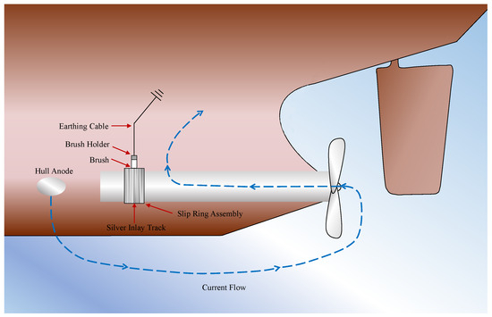
Figure 1.
The circuit formed by the anti-corrosion current between the hull and seawater.
When the propeller is running, because of the oil film thickness, bearing temperature, hull deformation and marine environment and other factors, the mechanical structure of the shaft connection produces a periodic change in contact resistance, so that the corrosion between the hull and seawater or corrosion circuit current changes, the circuit current is modulated to produce a propeller shaft-rate as the base frequency of the ELF electromagnetic field signals [24], known as the shaft-rate electromagnetic field. Because the electric field component of electromagnetic wave in seawater is easier to be detected than magnetic field, and the accuracy of detection instruments is also higher, so the detection is mainly based on the electric field signal. The shaft-rate electric field signal in seawater exhibits minimal attenuation, is challenging to suppress, and displays distinct line spectrum characteristics, making it a crucial signal source for detecting ships and underwater vehicles.
3. Methodology
3.1. Algorithm of VMD
The VMD algorithm employs iterative computation to derive the optimal solution of variational modes in the signal’s frequency domain and transforms the modal function along with the center frequency to derive the eigenmode function with varying bandwidths [25]. The fundamental steps to convert the signal modal estimation into a variational problem for resolution are outlined below. Decompose the original signal into K modal functions with a center frequency of , where K is the predetermined number of modes, and the modal function is represented as:
where: is the kth eigenmode function; and are the instantaneous amplitude and phase, respectively. The Hibert transform of yields the analytic signal and the one-sided spectrum ; the analytic signal is added to estimate the center frequency and the modal spectrum is converted to the fundamental band [26,27]; the squared L2 norm of the gradient of the analytic signal is calculated to estimate the bandwidth of the modal signal, transforming it into a constrained variational problem, and can be solved for the IMF of .
where: is the k IMF components obtained from signal decomposition; is the center frequency corresponding to each component; is the pulse function. The introduction of quadratic penalty coefficients and Lagrange multiplier operator in computing the constrained variational problem can be transformed into an unconstrained variational problem. The problem is further solved by alternating direction multiplier algorithm by alternately updating , and to solve the saddle points of the extended Lagrange expression to obtain the optimal solution.
where: is the Fourier transform of the original signal , is the Lagrange multiplier and is usually initialized to 0, is the penalty factor, which affects the bandwidth of the decomposition. The can be reconstructed from the superposition of the IMF components after decomposition:
where: represents the components of the decomposition and represents the residual after k levels of decomposition.
The VMD algorithm is adept at matching the optimal center frequency and finite bandwidth for each modal component, rendering it particularly suitable for the decomposition of shaft-rate electric field signals characterized by prominent harmonic features. During the next denoising process, we can accurately identify the signal’s frequency band, thereby removing noise and signal-free components to enhance denoising precision.
3.2. Algorithm of MSS
The spectral subtraction method is grounded on the assumption of additive noise [28,29], where the pristine signal is uncorrelated with the noise. By leveraging the short-time smoothness property of the noisy signal, the pure effective signal is derived through subtracting the short-time spectrum of the noise from that of the original data with noise. The frequency-domain data and its power spectrum are obtained by dividing the time-domain raw signals into time windows and then performing short-time Fourier transforms on of each time window:
where: , and are the frequency-domain data of the original signal, noise and effective signal, respectively; and are complex conjugates; and represent the short-time power spectra of the pure effective signal and noise, respectively; is the mutual correlation term, because the spectral subtraction method is based on the assumption of additive noise, i.e., there is no correlation between the pure effective signal and the noise, therefore, based on the assumption of additive noise in the spectral subtraction method, this term is 0. Transform Equation (6) to get the power spectrum of the pure effective signal. The power spectrum of the pure effective signal is obtained by transforming Equation (7):
expressed as:
where: is the amplitude spectrum of the signal with noise; is the phase spectrum of the signal with noise. expressed as:
where: is the amplitude spectrum of the noise; is the phase spectrum of the noise.Then take the square root of and bring the phase spectrum into it for the Fourier inverse transform, to obtain the pure effective signal of this time window, will be superimposed on all time windows to obtain the complete signal denoised effective signal.
The algorithm can effectively remove the background noise, but there are also defects [30], in the actual denoising process of the noise component of the larger time period will remain too large noise, in the spectrum for the random appearance of spikes, the interference of the pure signal is serious, so it must be suppressed. So in the classical spectral subtraction method on the basis of the introduction of multi-window spectral estimation method [31], the same data series with a number of orthogonal data windows were used to seek the data series of the magnitude spectrum and phase spectrum, and then averaged the obtained values to get the spectral estimation with a smaller variance. The definition of the multi-window spectral subtraction function is shown in Equation (10).
where: L is the number of data windows, is the noise spectrum with smaller estimation error; the spectrum of the kth data window:
where: N is the length of the sequence, is the kth data window function, and multiple data windows are orthogonal to each other:
In the formula, the frame serves as the central reference point, with M frames selected before and after it, resulting in a total of frames being averaged. Typically, we set the value of , which means we calculate the average of 3 adjacent frames. Repeating the process of spectral subtraction gives the final noise reduction signal:
The MSS algorithm, in comparison to threshold setting and bandpass filtering, fully utilizes the spectrum characteristics of environmental noise. The magnitude of noise in each frequency band is determined by the input noise sample, enabling the elimination of noise across multiple frequency bands and overcoming the challenge of manual threshold setting.Simultaneously, the power spectrum of electromagnetic noise in the actual ocean environment can be regarded as relatively constant within the observation window. For instance, the time-frequency traits of the induced electromagnetic field resulting from tides and seawater motion, as well as the electromagnetic field from seismic events, remain nearly constant over a brief temporal span, which improves the accuracy of the noise power estimation in the MSS algorithm.
3.3. Denoising Method Based on VMD-MSS
Addressing the characteristics of shaft-rate signals and electromagnetic noise in the marine environment, a noise reduction method is proposed by combining VMD and MSS. VMD generates modal components with center frequencies matching the spectral characteristics of the signal lines. Leveraging the smooth nature of marine electromagnetic noise within short time windows, noise removal is performed on different modes individually. Subsequently, the clean signal is reconstructed, enabling effective noise reduction and signal extraction even when signal and noise overlap in the same frequency band. The denoising process is divided into three main parts, and the comprehensive noise reduction flowchart of VMD-MSS is illustrated in Figure 2.

Figure 2.
The flowchart of VMD-MSS denoising method.
- (1)
- Preprocessing: the collected marine electromagnetic data are calibrated in advance, and then band-pass filtering is performed on the frequency band of the ship’s shaft-rate electric field signals, and the frequency band interval applied in this paper is 0.5∼20 Hz.
- (2)
- Decomposition: the noisy signal obtained by preprocessing is decomposed by VMD to get the IMFs of the signal with noise, set K = 5 (the smallest effective decomposition layer number for shaft-rate signal), = 2000. Respectively, each modal component for the extraction of noise intervals, the extraction of which can be intercepted using the method of Continuous Wavelet Transform (CWT) time-frequency analysis.
- (3)
- Denoising and reconstruction: the IMFs of the noisy signal and the IMFs of the noisy samples are subjected to multi-window spectral estimation, inter-frame smoothing and spectral subtraction noise reduction respectively to obtain the noise reduced IMFs, and the complete noise reduced signal is obtained by reconstruction.
4. Effectiveness Analysis
4.1. Simulation Analysis
In order to validate the effectiveness of the noise reduction method, the clean shaft-rate electric field signal with a fundamental frequency of 2 Hz, containing the 2nd and 3rd harmonics, is simulated, and the window duration is 10 s, i.e., 0 < t < 10, the signal starts from the 2 s and disappears in 8 s. The sampling rate is 50 Hz, the amplitude of the harmonics decreases with the increase of the order, the attenuation coefficient is , the change of the signal strength with time obeys the sinusoidal decay, and the signal peaks at the central time of 5 s, gradually diminishing towards both ends to mimic the scenario where the target progressively nears and then recedes during the detection process, resulting in a signal that initially amplifies and subsequently diminishes. The specific definitions of the simulated signals are as follows:
where, , k = 1, 2, 3, represent the order of the harmonics. Gaussian white noise was added to the simulated clean signal (Figure 3a) to generate a noisy signal (Figure 3b) with SNR of −5 dB, and the time series and CWT time-frequency plots are shown in Figure 3.
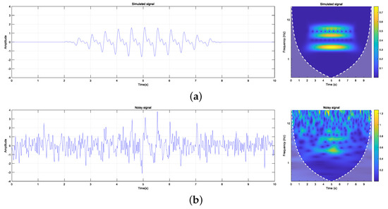
Figure 3.
The simulated clean signal and noisy signal.
Three algorithms (EMD, DWT, and VMD) were employed for modal decomposition, and the frequency band and energy distribution of different modal components were calculated, as shown in Table 1. Overlapping of frequency bands exists among different modes obtained by EMD, and the energy proportion of higher-order modes is minimal. While DWT addresses the frequency band overlap issue, it fails to rectify the low energy proportion of higher-order modes, and does not achieve the purpose of improving frequency resolution, which may hinder the effective utilization of noise features across different modes in the subsequent application of the MSS noise reduction algorithm, which is not conducive to noise removal.

Table 1.
Effects of different methods on the decomposition of noisy signals.
Upon analyzing the decomposition outcomes of VMD, it is evident that each mode has a narrower frequency band compared to the other two methods, particularly in IMF5, the frequency band width ranges from 1.53 Hz to 2.18 Hz, with an energy ratio of 40.96%, aligning closely with the 2 Hz fundamental frequency parameter set in the simulation. The lower-order mode also displays the frequency doubling phenomenon of the shaft-rate electric field signal. Figure 4 illustrates the modal component waveforms obtained by each method. Regarding the decomposition effect, the VMD algorithm excels in high-order modes, enabling detailed decomposition of signal and noise into distinct frequency bands, thereby enhancing the frequency resolution for subsequent processing.
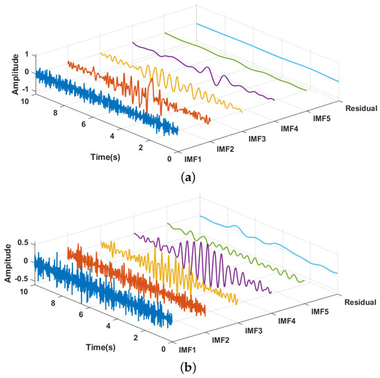

Figure 4.
Different decomposition methods and their mode functions: (a) EMD. (b) DWT. (c) VMD.
The results obtained by inputting the modal components decomposed by EMD, DWT and VMD and the undecomposed noise-containing signal into the MSS algorithm for noise reduction are shown in the Figure 5, the original noise-containing signal with a SNR = −5 is significantly improved after the noise reduction process, and the three decomposition methods combined with the MSS increase the SNR to 7.47 dB, 9.16 dB and 10.71 dB, respectively. 10.71 dB, and the signal without decomposition is only improved to 4.35 dB. It can be seen that the noise reduction effect of MSS can be significantly improved after modal decomposition, among which the denoising effect of VMD-MSS is most obvious.The denoised CWT time-frequency graphs are shown in Figure 6.

Figure 5.
Output waveforms and SNR of different denoising methods at SNR=−5.

Figure 6.
CWT time-frequency graphs of denoised signals output by different denoising methods: (a) EMD-MSS. (b) DWT-MSS. (c) VMD-MSS. (d) MSS.
By randomly generating 100 groups of simulated signals with different SNR, performing noise reduction processing, and statistically obtaining the distribution of their SNR enhancement effects, the result of denoising is shown in Figure 7, which shows that the SNR of the simulated signals have significant enhancement through denoising, especially at low SNR, the denoising method of VMD-MSS is still able to maintain a higher SNR enhancement effect.

Figure 7.
Results of SNR improvement using different methods.
4.2. Analysis of Measured Signal
In order to validate the noise reduction effectiveness of the VMD-MSS method on the measured electromagnetic data, we selected and processed experimental data collected in the northern waters of the South China Sea in June 2019. For a five-day observation test, three devices were deployed during this period. The recorded signals included a significant number of shaft-rate electric field signals generated by surface ship navigation and marine electromagnetic noise in the sea area. Figure 8 illustrates the Ocean Bed Electromagnetic (OBEM) acquisition station used in the testing process, while Figure 9 depicts the specific location of the test area situated at 17.83° N and 110.57° E in the South China Sea.

Figure 8.
The OBEM acquisition station used in the test.

Figure 9.
The field test location in the South China Sea.
The acquisition station is positioned on the seabed at a depth of 80 m to measure the signal produced by ship navigation through recording the potential difference between the two endpoints of the extended baseline. The sampling rate is 50 Hz, sufficient to capture the frequency spectrum of the shaft-rate electric field signal. The discrepancy between the cable length and the actual horizontal distance between its ends, influenced by seabed topography and navigational deviations, introduces some error. However, measured results indicate that the impact is small. Figure 10 illustrates the measured signal along with actual marine electromagnetic noise. Subsequent to feeding the modal components of the noisy signal into the MSS algorithm, Figure 11 displays the denoised modal components of different orders. The significant reduction of noise across various frequency bands is clearly evident.

Figure 10.
Measured signal with marine electromagnetic noise.
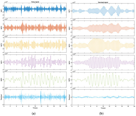
Figure 11.
Modal components after VMD decomposition: (a) Noisy signal. (b) Denoised signal.
Denoising each IMF component effectively eliminates noise across different frequency bands while preserving the signal’s line spectrum characteristics. As illustrated in Figure 12, the fundamental and octave frequencies, initially obscured by noise, are extracted, aligning with the signal features typical of ship navigation. Denoising processing has also been conducted on various other types of measured signals, with the results depicted in the Figure 13.

Figure 12.
Denoised signal waveform and CWT time-frequency diagram.

Figure 13.
The denoising effect of three different types of shaft-rate electric field signals.
Based on the processing outcomes of the measured signals, the VMD-MSS noise reduction technique exhibits robust stability across various signal and noise environments, effectively eliminating electromagnetic noise in the marine setting. To validate the noise reduction effectiveness of this method under low SNR conditions, various sets of measured signals with SNR levels of −5 dB, 0 dB, and 5 dB are chosen for denoising, and the output SNR and RMSE are shown in the Table 2. The MSS method without decomposition shows the smallest improvement in direct denoising, with the largest signal RMSE. This suggests that pre-decomposition of the signal is beneficial for enhancing the noise reduction effectiveness of the MSS algorithm. Among the three post-decomposition denoising methods, VMD-MSS demonstrates the most significant improvement, particularly at SNR values of 5 dB and 0 dB, surpassing other methods in denoising effectiveness and SNR enhancement.
Table 2.
Comparison of evaluation index with different methods.
The proposed denoising method demonstrates a favorable noise reduction effect on the measured signal, as evident from comparative analysis. It is apparent that VMD-MSS effectively eliminates electromagnetic noise in real marine environments and facilitates improved extraction of shaft-rate electric field signal characteristics.
5. Conclusions
A novel denoising method applicable to shaft-rate electric field signals is proposed based on the combination of VMD and MSS. The effectiveness of this method has been validated through simulation and experimental data. The advantages and conclusions of the VMD-MSS denoising method are as follows:
- (1)
- Through comparative analysis, VMD method can decompose the shaft-rate electric field signal more thoroughly. Compared with EMD and DWT method, the method used effectively avoids the problem of mode aliasing and improves the spectral resolution.
- (2)
- In comparison to EMD-MSS, DWT-MSS, and MSS, the VMD-MSS method exhibits SNR and lower RMSE in both simulated and experimental signal processing results. Particularly in low SNR scenarios, the noise reduction effectiveness of VMD-MSS is notably pronounced.
- (3)
- The denoising method of VMD-MSS can well retain the double frequency characteristics of the shaft-rate signal, and the damage to the signal characteristics is very small through the time-frequency analysis of CWT.
The VMD-MSS denoising method proposed herein effectively eliminate marine electromagnetic noise, facilitating the extraction and classification of ship shaft-rate electric field signals and enhancing underwater target detection, tracking, and recognition capabilities. Nonetheless, the analysis of noise reduction effects has been limited to a single sea trial dataset, necessitating further verification across various sea areas, conditions, and target types. Future research will focus on applying the denoising method to diverse signal sources and environmental noise scenarios to validate its efficacy comprehensively.
Author Contributions
Conceptualization, Y.W. and D.W.; methodology, Y.W.; software, Y.W.; validation, C.C., D.W. and J.L.; formal analysis, Z.Y.; investigation, L.Y.; resources, D.W.; data curation, C.C.; writing—original draft preparation, Y.W.; writing—review and editing, Y.W.; visualization, J.L.; supervision, D.W.; project administration, D.W.; funding acquisition, D.W. All authors have read and agreed to the published version of the manuscript.
Funding
This research was funded by The National Natural Science Foundation of China (NSFC) Joint Fund Project, grant number U2241201.
Informed Consent Statement
Not applicable.
Data Availability Statement
The data that support the findings of this study are available from the corresponding author, [Y.W.], upon reasonable request.
Acknowledgments
We give thanks to the Ocean University of China for the equipment and personnel support provided during the sea trials.
Conflicts of Interest
The authors declare no conflict of interest.
Abbreviations
List of abbreviation:
| Abbreviation | Definition |
| ELF | Extremely Low Frequency |
| IMF | Intrinsic Mode Function |
| EMD | Empirical Mode Decomposition |
| DWT | Discrete Wavelet Transform |
| VMD | Variational Mode Decompositio |
| SVMD | Successive Variational Mode Decomposition |
| MSS | Multi-window Spectral subtraction |
| CWT | Continuous Wavelet Transform |
| OBEM | Ocean-bed Electromagnetic |
| RMSE | Root Mean Square Error |
| SNR | Signal-to-noise Ratio |
References
- Yu, P.; Cheng, J.; Zhang, J. Ship target tracking using underwater electric field. Prog. Electromagn. Res. M 2019, 86, 49–57. [Google Scholar] [CrossRef]
- Bannister, P.R. ELF propagation update. IEEE J. Ocean. Eng. 1984, 9, 179–188. [Google Scholar] [CrossRef]
- Sun, Y.; Lin, C.; Jia, W.; Zhai, G. Analysis and measurement of ship shaft-rate magnetic field in air. Prog. Electromagn. Res. M 2016, 52, 119–127. [Google Scholar] [CrossRef]
- Weaver, J.T. The quasi-static field of an electric dipole embedded in a two-layer conducting halfspace. Can. J. Phys. 1967, 45, 1981–2002. [Google Scholar] [CrossRef]
- Wang, X.; Wang, S.; Hu, Y.; Tong, Y. Mixed Electric Field of Multi-Shaft Ship Based on Oxygen Mass Transfer Process under Turbulent Conditions. Electronics 2022, 11, 3684. [Google Scholar] [CrossRef]
- Lin, P.; Zhang, N.; Chang, M.; Xu, L. Research on the model and the location method of ship shaft-rate magnetic field based on rotating magnetic dipole. IEEE Access. 2020, 99, 162999–163005. [Google Scholar] [CrossRef]
- Schaefer, D.; Thiel, C.; Doose, J.; Rennings, A.; Erni, D. Above water electric potential signatures of submerged naval vessels. J. Mar. Sci. Eng. 2019, 7, 53. [Google Scholar] [CrossRef]
- Fares, S.A.; Fleming, R.; Dinn, D.; Purcell, C.J.T. Horizontal and vertical electric dipoles in a two-layer conducting medium. IEEE Trans. Antennas Propag. 2014, 62, 5656–5665. [Google Scholar] [CrossRef]
- Guibert, A.; Coulomb, J.-L.; Chadebec, O.; Rannou, C. Corrosion Diagnosis of a Ship Mock-Up from Near Electric-Field Measurements. IEEE Trans. Magn. 2010, 46, 3205–3208. [Google Scholar] [CrossRef]
- Kim, Y.S.; Lee, S.K.; Kim, J.G. Influence of anode location and quantity for the reduction of underwater electric fields under cathodic protection. Ocean Eng. 2018, 163, 476–482. [Google Scholar] [CrossRef]
- Jiang, C.; Lin, J.; Duan, Q.; Sun, S.; Tian, B. Statistical stacking and adaptive notch filter to remove high-level electromagnetic noise from MRS measurements. Surf. Geophys. 2011, 9, 459–468. [Google Scholar] [CrossRef]
- Jiang, W.; Ding, W.; Zhu, X.; Hou, F. A Recognition Algorithm of Seismic Signals Based on Wavelet Analysis. J. Mar. Sci. Eng. 2022, 10, 1093. [Google Scholar] [CrossRef]
- Birsan, M. Measurement of the extremely low frequency (ELF) magnetic field emission from a ship. Meas. Sci. Technol. 2011, 22, 085709. [Google Scholar] [CrossRef]
- Jia, Y.; Jiang, R.; Gong, S. Detection of ship shaft-rate electric field signal based on wavelet modulus maximum power. Acta Armamentarii Sin. 2013, 34, 592–596. [Google Scholar]
- Wang, G.; Wang, X.; Zhao, C. An iterative hybrid harmonics detection method based on discrete wavelet transform and Bartlett–Hann window. Appl. Sci. 2020, 10, 3922. [Google Scholar]
- Larsen, J.; Dalgaard, E.; Auken, E. Noise cancelling of MRS signals combining model-based removal of powerline harmonics and multichannel Wiener filtering. Geophys. J. Int. 2014, 196, 828–836. [Google Scholar] [CrossRef]
- Dalgaard, E.; Auken, E.; Larsen, J. Adaptive noise cancelling of multichannel magnetic resonance sounding signals. Geophys. J. Int. 2012, 191, 88–100. [Google Scholar] [CrossRef]
- Li, Y.; Zhang, C.; Zhou, Y. A Novel Denoising Method for Ship-Radiated Noise. J. Mar. Sci. Eng. 2023, 11, 1730. [Google Scholar] [CrossRef]
- Chen, X.; Zhao, X.; Liang, Y.; Luan, X. Ocean turbulence denoising and analysis using a novel EMD-based denoising method. J. Mar. Sci. Eng. 2022, 10, 663. [Google Scholar] [CrossRef]
- Yao, X.; Zhang, J.; Yu, Z.; Zhao, F.; Sun, Y. Random noise suppression of magnetic resonance sounding data with intensive sampling sparse reconstruction and kernel regression estimation. Remote Sens. 2019, 11, 1829. [Google Scholar] [CrossRef]
- Li, H.; Chang, J.; Xu, F.; Liu, Z.; Liu, B. Efficient lidar signal denoising algorithm using variational mode decomposition combined with a whale optimization algorithm. Remote Sens. 2019, 11, 126. [Google Scholar] [CrossRef]
- Li, C.; Wu, Y.; Lin, H.; Li, J.; Zhang, F.; Yang, Y. ECG denoising method based on an improved VMD algorithm. IEEE Sens. J 2022, 22, 22725–22733. [Google Scholar] [CrossRef]
- Zolotarevskii, Y.M.; Bulygin, F.V.; Ponomarev, A.N.; Narchev, V.A. Methods of measuring the low-frequency electric and magnetic fields of ships. Meas. Tech. 2005, 48, 1140–1144. [Google Scholar] [CrossRef]
- Traverso, P.; Canepa, E. A review of studies on corrosion of metals and alloys in deep-sea environment. Ocean Eng. 2014, 87, 10–15. [Google Scholar] [CrossRef]
- Dragomiretskiy, K.; Zoss, D. Variational Mode Decomposition. IEEE Trans. Signal Process. 2014, 62, 531–544. [Google Scholar] [CrossRef]
- Li, Q.; Li, J.; Shi, Z.; Li, Z.; Wen, X. An improved VMD method for MGTS calibration and target tracking. IEEE Sens. J. 2023, 23, 27984–27996. [Google Scholar] [CrossRef]
- Yan, F.; Pi, S.; Qi, Y.; Lin, J. Transient electromagnetic data noise suppression method based on RSA-VMD-DNN. IEEE Geosci. Remote Sens. Lett. 2024, 21, 7500105. [Google Scholar] [CrossRef]
- Boll, S. Suppression of acoustic noise in speech using spectral subtraction. IEEE Trans. Acoust. Speech Signal Process. 1979, 27, 113–120. [Google Scholar] [CrossRef]
- Yadava, T.; Nagaraja, B.G. A spatial procedure to spectral subtraction for speech enhancement. Multimed Tools Appl. 2022, 81, 23633–23647. [Google Scholar]
- Dash, T.K.; Solanki, S.S. Speech intelligibility based enhancement system using modified deep neural network and adaptive multi-band spectral subtraction. Ocean Eng. 2020, 111, 1073–1087. [Google Scholar] [CrossRef]
- Lin, T.; Yao, X.; Yu, S.; Zhang, Y. Electromagnetic noise suppression of magnetic resonance sounding combined with data acquisition and multi-frame spectral subtraction in the frequency domain. Electronics 2020, 9, 1254. [Google Scholar] [CrossRef]
Disclaimer/Publisher’s Note: The statements, opinions and data contained in all publications are solely those of the individual author(s) and contributor(s) and not of MDPI and/or the editor(s). MDPI and/or the editor(s) disclaim responsibility for any injury to people or property resulting from any ideas, methods, instructions or products referred to in the content. |
© 2024 by the authors. Licensee MDPI, Basel, Switzerland. This article is an open access article distributed under the terms and conditions of the Creative Commons Attribution (CC BY) license (https://creativecommons.org/licenses/by/4.0/).