


Joint Inversion of Sea Surface Wind and Current Velocity Based on Sentinel-1 Synthetic Aperture Radar Observations


Abstract
1. Introduction
2. Data and Method
2.1. Sentinel-1
2.2. ECMWF Winds
2.3. Buoy Winds
2.4. High-Frequency Radar
2.5. Drifter Current Velocity
2.6. CMOD7 and CDOP
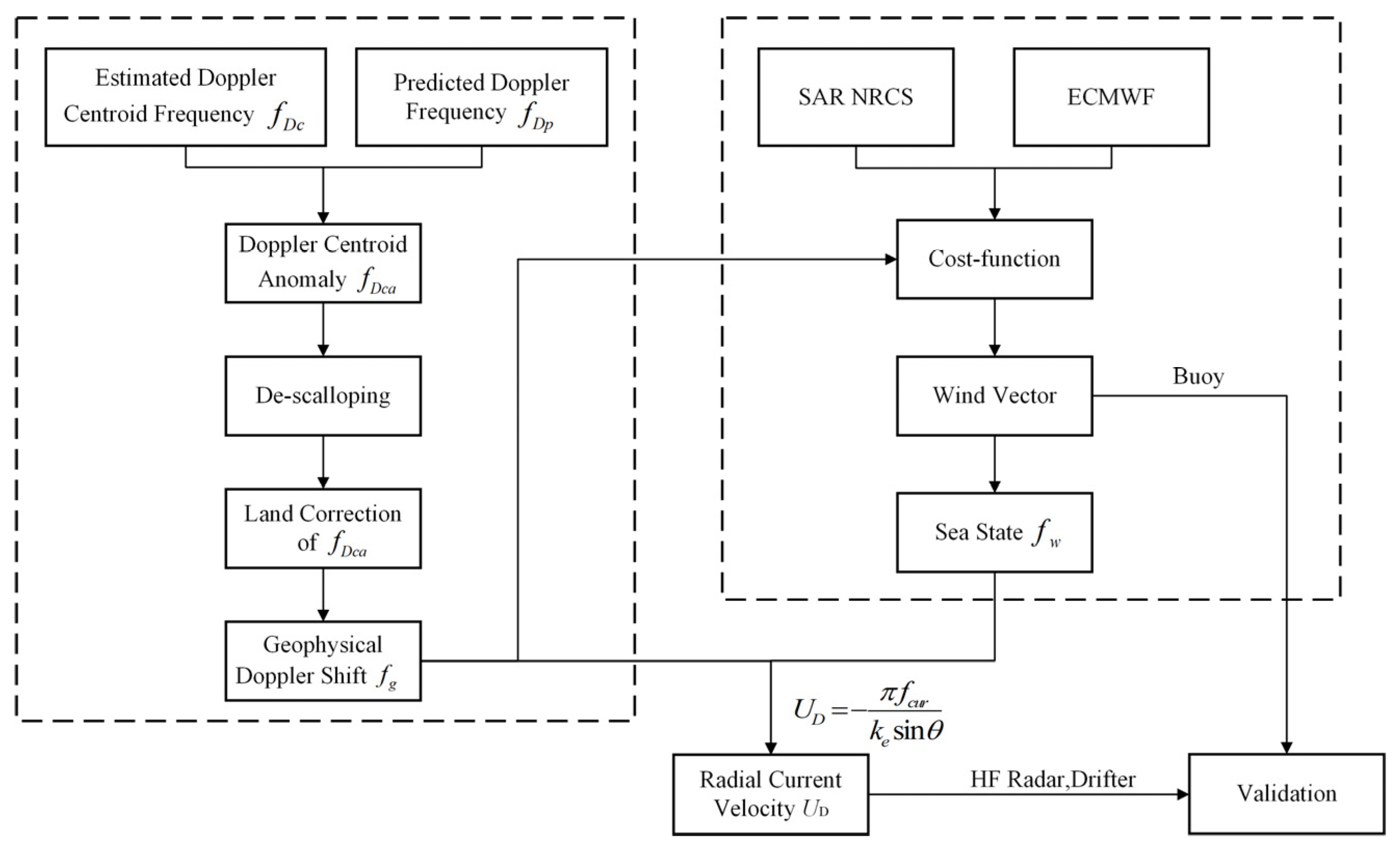
2.7. Method
3. Results and Discussions
3.1. DCA Correction
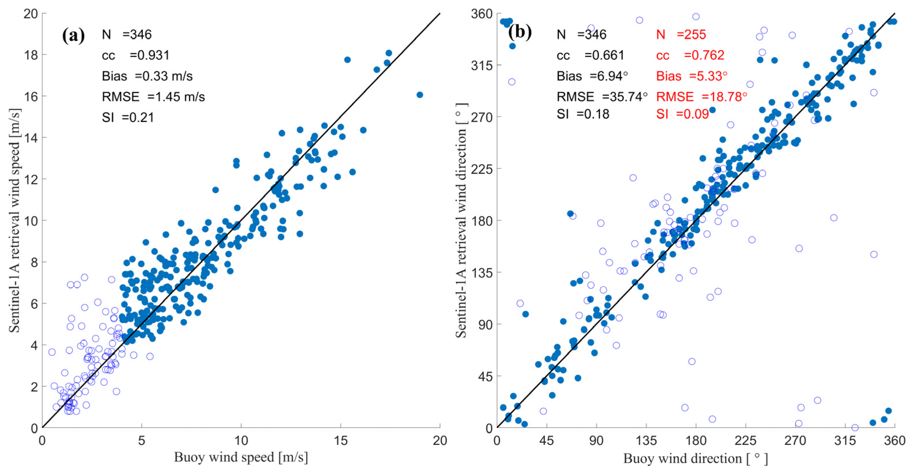
3.2. Wind Retrieval and Validation
3.3. Current Retrieval and Validation
4. Summary
Author Contributions
Funding
Institutional Review Board Statement
Informed Consent Statement
Data Availability Statement
Acknowledgments
Conflicts of Interest
References
- Durand, M.; Fu, L.-L.; Lettenmaier, D.P.; Alsdorf, D.E.; Rodriguez, E.; Esteban-Fernandez, D. The surface water and ocean topography mission: Observing terrestrial surface water and oceanic submesoscale eddies. Proc. IEEE 2010, 98, 766–779. [Google Scholar] [CrossRef]
- Bourassa, M.A.; Meissner, T.; Cerovecki, I.; Chang, P.S.; Dong, X.L.; De Chiara, G.; Donlon, C.; Dukhovskoy, D.S.; Elya, J.; Fore, A.; et al. Remotely Sensed Winds and Wind Stresses for Marine Forecasting and Ocean Modeling. Front. Mar. Sci. 2019, 6, 443. [Google Scholar] [CrossRef]
- He, Y.; Liu, B.; Zhang, B.; Cheng, Z.; Qiu, Z. Overview on satellite remote-sensing methods for sea-surface-current measurement. Guangxi Sci. 2015, 22, 294–300. [Google Scholar] [CrossRef]
- Stoffelen, A.; Anderson, D. Scatterometer data interpretation: Estimation and validation of the transfer function CMOD4. J. Geophys. Res. Ocean. 1997, 102, 5767–5780. [Google Scholar] [CrossRef]
- Ju-Hong, Z.; Ming-Sen, L.; De-Lu, P.; Zheng-Hua, C.; Le, Y. A unified C-band and Ku-band GMF determined by using neural network approach. Acta Oceanol. Sin. 2008, 30, 23–28. [Google Scholar] [CrossRef]
- Zecchetto, S.; De Biasio, F.; della Valle, A.; Quattrocchi, G.; Cadau, E.; Cucco, A. Wind Fields From C- and X-Band SAR Images at VV Polarization in Coastal Area (Gulf of Oristano, Italy). IEEE J. Sel. Top. Appl. Earth Observ. Remote Sens. 2016, 9, 2643–2650. [Google Scholar] [CrossRef]
- Du, Y.; Dong, X.; Jiang, X.; Zhang, Y.; Zhu, D.; Sun, Q.; Wang, Z.; Niu, X.; Chen, W.; Zhu, C. Ocean Surface Current multiscale Observation Mission (OSCOM): Simultaneous measurement of ocean surface current, vector wind, and temperature. Prog. Oceanogr. 2021, 193, 102531. [Google Scholar] [CrossRef]
- Qiu, B.; Chen, S.; Klein, P.; Torres, H.; Wang, J.; Fu, L.; Menemenlis, D. Reconstructing Upper-Ocean Vertical Velocity Field from Sea Surface Height in the Presence of Unbalanced Motion. J. Phys. Oceanogr. 2020, 50, 55–79. [Google Scholar] [CrossRef]
- Keller, W.; Plant, W.; Valenzuela, G. Observation of breaking ocean waves with coherent microwave radar. In Wave Dynamics and Radio Probing of the Ocean Surface; Springer: Boston, MA, USA, 1986; pp. 285–293. [Google Scholar] [CrossRef]
- Horstmann, J.; Koch, W.; Lehner, S.; Tonboe, R. Ocean winds from RADARSAT-1 ScanSAR. Can. J. Remote Sens. 2002, 28, 524–533. [Google Scholar] [CrossRef]
- Monaldo, F.; Thompson, D.; Beal, R.; Pichel, W.; Clemente-Colon, P. Comparison of SAR-derived wind speed with model predictions and ocean buoy measurements. IEEE Trans. Geosci. Remote Sens. 2001, 39, 2587–2600. [Google Scholar] [CrossRef]
- Mouche, A.; Collard, F.; Chapron, B.; Dagestad, K.; Guitton, G.; Johannessen, J.; Kerbaol, V.; Hansen, M. On the Use of Doppler Shift for Sea Surface Wind Retrieval From SAR. IEEE Trans. Geosci. Remote Sens. 2012, 50, 2901–2909. [Google Scholar] [CrossRef]
- Chapron, B.; Collard, F.; Ardhuin, F. Direct measurements of ocean surface velocity from space: Interpretation and validation. J. Geophys. Res. Ocean. 2005, 110, 17. [Google Scholar] [CrossRef]
- Hansen, M.W.; Collard, F.; Dagestad, K.F.; Johannessen, J.A.; Fabry, P.; Chapron, B. Retrieval of Sea Surface Range Velocities From Envisat ASAR Doppler Centroid Measurements. IEEE Trans. Geosci. Remote Sens. 2011, 49, 3582–3592. [Google Scholar] [CrossRef]
- Rouault, M.J.; Mouche, A.; Collard, F.; Johannessen, J.A.; Chapron, B. Mapping the Agulhas Current from space: An assessment of ASAR surface current velocities. J. Geophys. Res. Ocean. 2010, 115, 14. [Google Scholar] [CrossRef]
- Kang, K.; Kim, D.j.; Kim, S.H.; Moon, W. Doppler Velocity Characteristics During Tropical Cyclones Observed Using ScanSAR Raw Data. IEEE Trans. Geosci. Remote Sens. 2016, 54, 2343–2355. [Google Scholar] [CrossRef]
- Bao, Q. System Design and Simulation of Doppler Scatterometer—Wide Swath Ocean Surface Current Measurement. Department of Electromagnetic Field and Microwave Technology. Ph.D. Thesis, University of Chinese Academy of Sciences, Beijing, China, 2015. [Google Scholar]
- Moiseev, A.; Johannessen, J.A.; Johnsen, H. Towards Retrieving Reliable Ocean Surface Currents in the Coastal Zone From the Sentinel-1 Doppler Shift Observations. J. Geophys. Res. Ocean. 2022, 127, e2021JC018201. [Google Scholar] [CrossRef]
- Martin, A.C.; Gommenginger, C.P.; Jacob, B.; Staneva, J. First multi-year assessment of Sentinel-1 radial velocity products using HF radar currents in a coastal environment. Remote Sens. Environ. 2022, 268, 112758. [Google Scholar] [CrossRef]
- Eyre, J.R.; English, S.J.; Forsythe, M. Assimilation of satellite data in numerical weather prediction. Part I Early Years. Q. J. R. Meteorol. Soc. 2020, 146, 49–68. [Google Scholar] [CrossRef]
- Elipot, S.; Lumpkin, R.; Perez, R.C.; Lilly, J.M.; Early, J.J.; Sykulski, A.M. A global surface drifter data set at hourly resolution. J. Geophys. Res. Oceans 2016, 121, 2937–2966. [Google Scholar] [CrossRef]
- Stoffelen, A.; Verspeek, J.A.; Vogelzang, J.; Verhoef, A. The CMOD7 geophysical model function for ASCAT and ERS wind retrievals. IEEE J. Sel. Top. Appl. Earth Observ. Remote Sens. 2017, 10, 2123–2134. [Google Scholar] [CrossRef]
- Elyouncha, A.; Eriksson, L.E.B.; Johnsen, H.; Ulander, L.M.H. Using Sentinel-1 Ocean Data for Mapping Sea Surface Currents Along the Southern Norwegian Coast. In Proceedings of the IGARSS 2019—2019 IEEE International Geoscience and Remote Sensing Symposium, Yokohama, Japan, 28 July–2 August 2019; pp. 8058–8061. [Google Scholar] [CrossRef]
- Hajduch, G.; Vincent, P.; Piantanida, R.; Recchia, A.; Franceschi, N.; Schmidt, K.; Johnsen, H.; Mouche, A.; Grouazel, A.; Collard, F. Sentinel-1 A and B Annual Performance Report for 2020; Tech. Rep. MPC-0504; Mission Performance Center, ESA: Paris, France, 2021. [Google Scholar]
- Hoffman, R.; Leidner, S.; Henderson, J.; Atlas, R.; Ardizzone, J.; Bloom, S. A two-dimensional variational analysis method for NSCAT ambiguity removal: Methodology, sensitivity, and tuning. J. Atmos. Ocean. Technol. 2003, 20, 585–605. [Google Scholar] [CrossRef]
- Portabella, M.; Stoffelen, A.; Johannessen, J.A. Toward an optimal inversion method for synthetic aperture radar wind retrieval. J. Geophys. Res. Ocean. 2002, 107, 1–13. [Google Scholar] [CrossRef]
- Elyouncha, A.; Eriksson, L.E.; Broström, G.; Axell, L.; Ulander, L.H. Joint retrieval of ocean surface wind and current vectors from satellite SAR data using a Bayesian inversion method. Remote Sens. Environ. 2021, 260, 112455. [Google Scholar] [CrossRef]
- Li, X.-M.; Qin, T.; Wu, K. Retrieval of Sea Surface Wind Speed from Spaceborne SAR over the Arctic Marginal Ice Zone with a Neural Network. Remote Sens. 2020, 12, 3291. [Google Scholar] [CrossRef]


| Variable | Metrics | NRCS + Model | NRCS + Model + Doppler |
|---|---|---|---|
| Wind speed | Bias [m/s] | 0.34 | 0.33 |
| RMSE [m/s] | 1.45 | 1.45 | |
| Wind direction | Bias [°] | 7.25 | 6.94 |
| RMSE [°] | 35.84 | 35.74 |
Disclaimer/Publisher’s Note: The statements, opinions and data contained in all publications are solely those of the individual author(s) and contributor(s) and not of MDPI and/or the editor(s). MDPI and/or the editor(s) disclaim responsibility for any injury to people or property resulting from any ideas, methods, instructions or products referred to in the content. |
© 2024 by the authors. Licensee MDPI, Basel, Switzerland. This article is an open access article distributed under the terms and conditions of the Creative Commons Attribution (CC BY) license (https://creativecommons.org/licenses/by/4.0/).
Share and Cite
Sun, J.; Li, H.; Lin, W.; He, Y. Joint Inversion of Sea Surface Wind and Current Velocity Based on Sentinel-1 Synthetic Aperture Radar Observations. J. Mar. Sci. Eng. 2024, 12, 450. https://doi.org/10.3390/jmse12030450
Sun J, Li H, Lin W, He Y. Joint Inversion of Sea Surface Wind and Current Velocity Based on Sentinel-1 Synthetic Aperture Radar Observations. Journal of Marine Science and Engineering. 2024; 12(3):450. https://doi.org/10.3390/jmse12030450
Chicago/Turabian StyleSun, Jingbei, Huimin Li, Wenming Lin, and Yijun He. 2024. "Joint Inversion of Sea Surface Wind and Current Velocity Based on Sentinel-1 Synthetic Aperture Radar Observations" Journal of Marine Science and Engineering 12, no. 3: 450. https://doi.org/10.3390/jmse12030450
APA StyleSun, J., Li, H., Lin, W., & He, Y. (2024). Joint Inversion of Sea Surface Wind and Current Velocity Based on Sentinel-1 Synthetic Aperture Radar Observations. Journal of Marine Science and Engineering, 12(3), 450. https://doi.org/10.3390/jmse12030450