Article

Multi-Module Fusion Model for Submarine Pipeline Identification Based on YOLOv5

1
School of Surveying and Geoinformation Engineering, East China University of Technology, Nanchang 330013, China
2
Key Laboratory of Mine Environmental Monitoring and Improving around Poyang Lake of Ministry of Natural Resources, East China University of Technology, Nanchang 330013, China
*
Author to whom correspondence should be addressed.
J. Mar. Sci. Eng. 2024, 12(3), 451; https://doi.org/10.3390/jmse12030451
Submission received: 3 February 2024 / Revised: 26 February 2024 / Accepted: 26 February 2024 / Published: 3 March 2024

Abstract

:
In recent years, the surge in marine activities has increased the frequency of submarine pipeline failures. Detecting and identifying the buried conditions of submarine pipelines has become critical. Sub-bottom profilers (SBPs) are widely employed for pipeline detection, yet manual data interpretation hampers efficiency. The present study proposes an automated detection method for submarine pipelines using deep learning models. The approach enhances the YOLOv5s model by integrating Squeeze and Excitation Networks (SE-Net) and S2-MLPv2 attention modules into the backbone network structure. The Slicing Aided Hyper Inference (SAHI) module is subsequently introduced to recognize original large-image data. Experimental results conducted in the Yellow Sea region demonstrate that the refined model achieves a precision of 82.5%, recall of 99.2%, and harmonic mean (F1 score) of 90.0% on actual submarine pipeline data detected using an SBP. These results demonstrate the efficiency of the proposed method and applicability in real-world scenarios.

1. Introduction

Subsea pipelines serve as conduits for transporting petroleum, natural gas, and high-voltage electrical currents. Severe malfunctions in the pipelines can result in significant economic losses and even pose threats to human life [1]. The causes of subsea pipeline failures can be attributed to two main factors. The first category includes mechanical damage resulting from human activities such as fishing, ship anchoring, and other related factors. Secondly, the deployment of cable pipelines in underwater terrains characterized by rugged features such as trenches and rocky substrates can lead to anomalies like pipeline exposure and suspension. Also, prolonged exposure to seawater in such conditions can contribute to the deterioration and damage of the pipeline [2].
To mitigate the risks of subsea pipeline failures such as leakage, rupture, and other hazards, regular pipeline inspections and maintenance are crucial [3,4]. However, because most subsea pipelines are located beneath the seabed, conventional measurement methods such as sonar and multibeam techniques, typically employed at shallower depths, are no longer applicable [5,6]. A sub-bottom profiler (SBP), as a sonar system based on the principles of underwater acoustics, serves as a continuous traverse-type detector for exploring sub-seabed geological structures and formations. Leveraging its lower transmission frequency, the SBP allows acoustic signals to penetrate through the water column, traverse the seabed, and further penetrate deeper layers of the seabed. Through geological analysis, the SBP facilitates the detection of structures and formations in the sub-seabed shallow layers. Also, the subsea profiling system can map the depositional structure of shallow sub-bottom layers through acoustic profile images. In addition to detecting exposed and suspended pipelines, the SBP can identify buried pipelines and hence provide extensive applications in underwater pipeline surveys [7,8].
In practical measurements, the measurement principle based on the SBP requires a perpendicular orientation to the pipeline direction in order to fully capture the pipeline information. Many researchers have investigated the detection of underwater pipelines from different directions. Karimanzira et al. [9] proposed a multi-sensor combination detection method for underwater pipeline detection using a multibeam echo sounder (MBES), SBP, and magnetic sensor. Lv et al. [10] proposed a method for recognizing submarine cable faults based on FCN-55 GRU-SVM. The method combines deep learning with experimental data from finite element simulations. Bharti et al. [11] utilized a magnetometer and Kalman filter for detecting subsea pipelines, aiming at pipeline positioning. However, the approach has limitations, such as low detection efficiency and inability to work with other sensors. Li et al. [12] employed an edge extraction method for pipeline localization, achieving a high-correct detection rate but with slower computational efficiency. Guan et al. [13] integrated a sub-bottom profiler with a ship-borne underwater multi-sensor mapping system aboard a vessel. The team developed a method for correcting position deviations to improve the precision of pipeline detection and localization. However, the data processing still relies on manual interpretation, leading to results influenced significantly by the operator’s experience, often resulting in misjudgments and omissions. Another drawback is the limited attention to the automated detection of subsea pipelines. Considering various imaging factors, pipeline shapes exhibit considerable variations in SBP images, posing challenges in feature extraction and complicating the automatic detection of subsea pipelines [14]. For this reason, the development of an automated and resilient approach for pipeline detection using SBP images is an urgent and pivotal concern. In addressing this problem and substantially reducing manual efforts while improving detection efficiency, this study incorporates deep learning techniques in pipeline automatic detection. Deep learning, leveraging its powerful feature learning capabilities and the ability to extract meaningful information from complex data, is introduced in the automated detection of pipelines [15]. Deep learning algorithms have demonstrated significant success in various tasks and domains, attributed to their generalization capability, adaptability, and scalability [16]. Li et al. [17], employing the YOLO V3 technique, demonstrated significant outcomes in the detection of underwater targets such as sunken ships, fish schools, and seafloor topography. The team accomplished the results by integrating spatial pyramid pooling and online dataset preprocessing. Chen et al. [18] improved the model’s sensitivity to channel features and enhanced target recognition by adjusting parameters and computational quantities in the Involution Bottleneck and incorporating an SE module. Despite the advantages, deep learning presents challenges such as dependency on large-scale annotated data and the opacity of the model. Yang et al. [19], demonstrated improved small object detection performance in the YOLOX model by refining it with Slicing Aided Hyper Inference SAHI. Keles et al. [20] investigated the integration of SAHI with YOLOv5 and YOLOX models, leading to a substantial improvement in optimizing the efficiency of the target detection model.
Considering substantial collection costs and difficulties associated with acquiring SBP data, it is often scarce and challenging to meet the training requirements of models. Also, common SBP images typically possess large dimensions, while pipeline images, characterized by simple structures, occupy a relatively small area within the SBP images. This implies the need to design a detection strategy capable of identifying small targets on large images to achieve rapid and accurate pipeline detection. This research adjusts the foundational network structure of the YOLO model, modifying the comprehensive attention mechanism to intensify the model’s focus on targets. The SAHI module is employed to segment large images into n 640 × 640-sized images for validation. The results are further combined by concatenating them to restore the original image size, displaying the predicted outcomes. This improvement enables the model to achieve satisfactory results when trained on a small dataset. By leveraging the optimal model proposed in this study and the SAHI module, the recognition of actual measurement data images is performed, which significantly reduces manual identification time and boosts data processing efficiency.

2. Experimental Data and Model

2.1. Experimental Background

The data collection site for this experiment is located offshore near Dafeng District and Xiangshui County, Jiangsu Province, China. Based on the geological information revealed through the borehole drilling, including the stratigraphic structure, lithological characteristics, burial conditions, and regional geological data, it is observed that within the exploration depth (with the deepest borehole reaching 77.00 m and an elevation of −91.66 m), the sediments belong to Quaternary deposits. The deposits are generally stratified as silt layers, fine sand layers, clay layers, and other marine sediments. Figure 1a,b depicts the study area map and the seafloor geological classification map, respectively.

2.2. Experimental Equipment

The equipment utilized for the shallow sub-bottom profile data collection was the SES-2000 Standard High-Resolution Shallow Sub-bottom Profiler, manufactured by the German company Innomar. This equipment is employed for transverse profiling operations of subsea pipelines. The operational water depth range of the equipment is 0.5 m to 500 m, with a penetration depth of less than 50 m and a resolution of greater than 5 cm. The post-processing software used for shallow profiling data and graphical operations was the Innomar ISE 2.9.5 analysis software. The computer setup for model execution consists of a system running Windows 11 with an Intel Core i7-12650H processor, NVIDIA GeForce RTX 4060 laptop GPU(Intel Corporation Headquarters City: Santa Clara, California, United States Country: United States), Python version 3.9, CUDA version 11.1, Conda version 23.7.4, PyTorch version 1.9.1+cu111, and a 12th generation Intel(R) Core(TM) i7-12650H CPU. The detailed configuration is shown in Table 1.

2.3. Data Preprocessing

The principle of SBP measurement data is to transmit acoustic pulses to the seafloor, where the acoustic wave encounters the acoustic impedance interface as it propagates through the seawater and sediment layers; part of the acoustic wave is reflected and returned to the transducer to be converted into analog or digital signals, then recorded and output as a shallow stratigraphic acoustic recording profile that can reflect the acoustic characteristics of the strata.
The data in this paper were collected using the SES-2000 Sub-bottom Profilera and post-processing using the ISE 2.9.5 software. The signal underwent steps such as seabed line tracking, gain compensation, and dynamic filtering compression to draw pixels based on intensity. After processing, the data were cropped to obtain 11,625 original images. Manual annotation using the labeling tool was performed to mark the position of the pipelines in each image with rectangular bounding boxes, resulting in text-formatted annotation files. During this process, manual cleaning of the dataset was conducted. The final pipeline dataset consisted of 1233 images. Before feeding these images into the enhanced YOLOv5 network model, the mosaic data augmentation technique was used to enrich the image dataset. This involved using strategies such as random resizing, arbitrary cropping, and random rearrangement for concatenating images, thereby effectively enlarging the dataset and enhancing the model’s aptitude for detecting diminutive targets. Before training the model, adaptive scaling and padding operations were performed on the subsea pipeline images to normalize the input image size to 640 × 640 pixels. Following labeling, the dataset was randomly divided into training, validation, and test sets in an 8:1:1 ratio. The training set was used to train the model, the validation set was used to evaluate the recognition performance of the model in each iteration, and optimized model files were saved. The test set was then used to evaluate the accuracy of the optimized model. The flowchart illustrating the proposed method is shown in Figure 2.

2.4. Experimental Model

The YOLOv5s model, as a lightweight model, consists mainly of three components: backbone, neck, and head [21]. After the image input is finalized, the backbone segment conducts feature extraction on the input images. The neck section is responsible for integrating features from multiple scales within the feature maps and transmitting these fused features to the prediction layer. The head segment performs regression predictions on image features, producing bounding boxes, and predicting categories. Based on variations in network depth and width, YOLOv5 can be classified into four model versions: YOLOv5s, YOLOv5m, YOLOv5l, and YOLOv5x. YOLOv5s as a small model has fewer network layers and parameters, is faster and less demanding on computational resources, and is suitable for scenarios with higher speed requirements. The YOLOv5m is a medium model, which has more network depths and widths than the YOLOv5s, and is therefore more accurate, but slightly slower. The YOLOv5l is a large model that adds more convolutional layers and more feature channels. It also provides higher detection accuracy, but runs at a lower speed compared to the YOLOv5s and YOLOv5m model versions. It is suitable for application scenarios that require higher accuracy and have some computing power environment. The YOLOv5x is a super large model with the largest network width and depth. It has the highest accuracy, but is the slowest and requires a lot of computing resources to support it. The YOLOv5 network uses the Generalized Intersection over Union (GIOU) as its network loss function, as shown in Equations (1) and (2).
G I O U = I O U C ( A B ) c ,
I O U = A B / A B ,
In this scenario, A and B denote any two bounding boxes, and C is a minimal enclosing box that can encompass both A and B. The GIOU is defined as the Intersection over Union (IOU) subtracted by the ratio of the area in C not covered by A and B to the total area of C.
The attention mechanism is inspired by the human visual attention system, which focuses on local information to suppress unnecessary details. This mechanism enables the network to extract meaningful information from a large amount of data. Attention mechanisms are mainly classified into spatial attention mechanisms and channel attention mechanisms. Channel attention mechanisms include SE-Net, the Convolutional Block Attention Module (CBAM), and Efficient Channel Attention (ECA-NET) in deep convolutional neural networks. Spatial attention mechanisms include self-attention, non-local attention, and other variants. In the context of lightweight networks, channel attention mechanisms generally exhibit more effective model enhancement compared to spatial attention mechanisms.
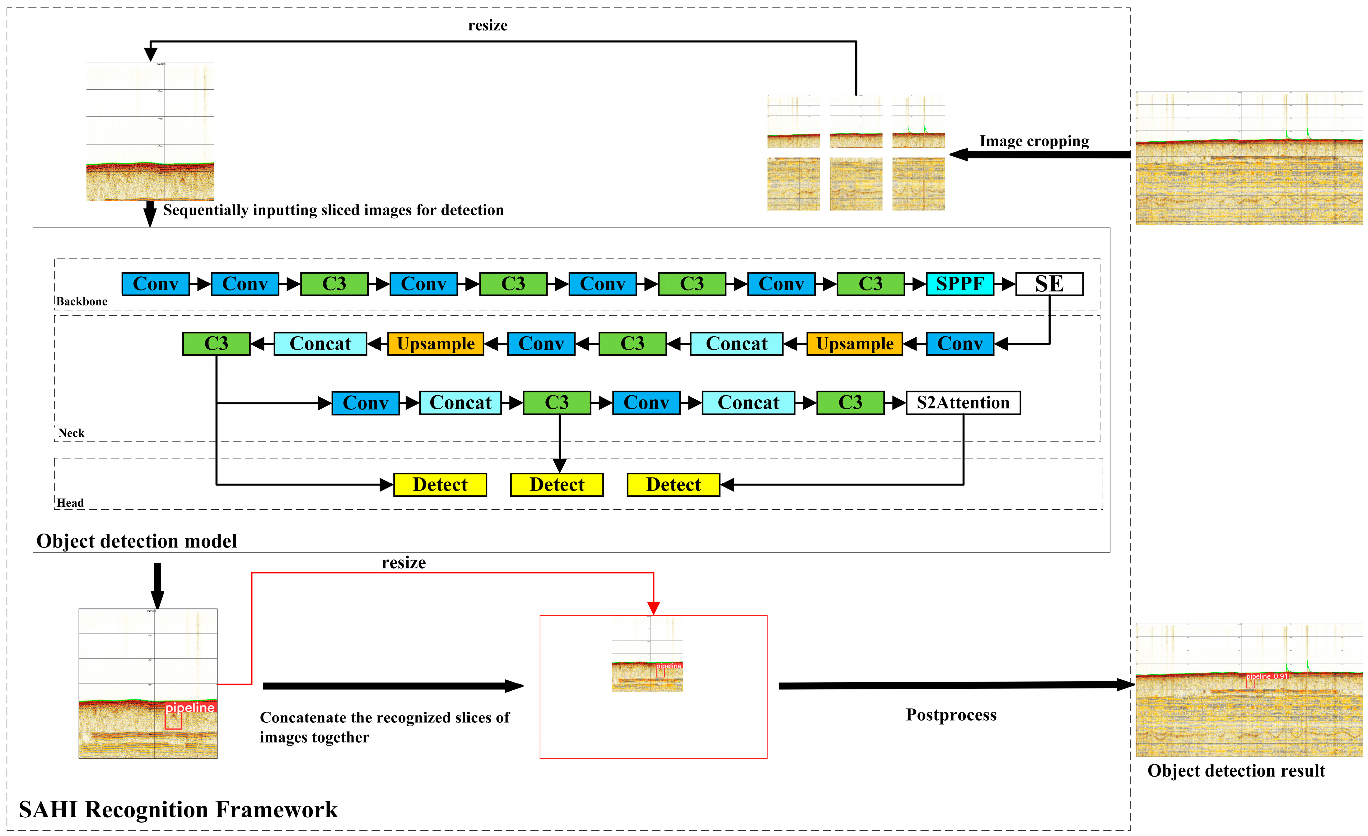
This study incorporated various attention models, including coordinate attention (CA), SE-Net, and S2Attention, into the backbone of YOLOv5s. Comparative assessments were conducted against other baseline models to evaluate detection performance and identify the network model with high accuracy for underwater pipeline identification. The altered network processing flow, incorporating CA, SE, and S2Attention attention in the network architecture, is depicted in Figure 3 [22,23,24].
In the CA module of this model, attention processing involves obtaining two one-dimensional vectors by applying separate average pooling operations in the horizontal and vertical directions. Concatenation and convolution operations are used to compress the channels in the spatial dimension. Spatial information in the vertical and horizontal directions is encoded through batch normalization (BN) and non-linear transformations. Following this, a split operation is conducted, and each segment is individually processed through a 1 × 1 Convolution to align with the channel number of the input image. The outcomes are then normalized and weighted, effectively amalgamating spatial information by assigning weights across channels. The CA module accomplishes spatial information fusion through horizontal and vertical average pooling, succeeded by spatial encoding and ultimately integrating spatial information through weighted channel-wise aggregation [24].
The SE-Net module uses Global Average Pooling to compress the input feature map into a one-dimensional vector. Weight coefficients are generated through two fully connected layers and ReLU activation functions, representing the importance of each channel. These weight coefficients are multiplied back into the original feature map, enhancing crucial features and attenuating less important ones. In this model, the SE-Net module functions as an attention mechanism, weighting across channels in the feature map dimension, effectively reweighting the input feature map to obtain the desired feature map.
For the S2-MLPv2 module in this study, the feature map is first expanded and divided into three parts. Each part undergoes separate transformations before being merged using scattered attention on the segmented feature maps. Hierarchical pyramids are employed to enhance the modeling capacity for fine-grained details, thereby achieving higher recognition accuracy. When SE-Net and S2-MLPv2 are added at different positions in the network, their impacts on the model differ, and in some instances, their accuracy may even be compromised. After multiple experiments, it was observed that incorporating SE-Net in the last layer of the backbone and S2-MLPV2 in the last layer of the head yielded better results.
In the conclusive experiment, the genuine data were validated using SAHI, an open-source detection method introduced by Fatih et al. [25] to address challenges in detecting small objects. SAHI is a method for object detection and instance segmentation models, characterized by slicing-assisted inference. This technique is implemented through image cropping and processing during the inference phase. The model was trained using a dataset collected in the field. The images are sequentially cropped to a size of 640 × 640 for recognition. The recognized images are then merged with the original size, which enables better recognition of small target objects on large-scale maps. During the experiment, the model threshold was set to 0.8, with slice length and width sizes set to 640. The length and width overlap of the next slice were set to 20%. The trained model weights were used to assign values to the detection model, improving the recognition performance of SAHI. Figure 4 shows the flowchart of the detection process after integrating the SAHI module.

3. Experimental Results and Analysis

This section lists the metrics related to evaluating the pipeline identification performance of the model, including precision, recall, AP (Average Precision), [email protected], and F1. Mathematical expressions for these metrics are shown in Equations (3) to (7).
P = T P T P + F P ,
R = T P T P + F N ,
F 1 = 2 × P × R P + R ,
A P = 0 1 P ( R ) d R = k = 0 n P ( k ) Δ R ( k ) ,
m A P = i = 1 C A P i C
In the provided definitions, P represents precision, R denotes recall, F1 is the harmonic mean of P and R, and AP is the average precision, indicating the average precision at various recall points or the area under the PR curve. The mean average precision (mAP) is the average of average precisions (APs) across multiple object categories, where C represents the number of categories. In this experiment, [email protected] corresponds to the average AP when the intersection-over-union threshold is set to 0.5. As there is only one category for this subject, mAP is equivalent to AP. FP (false positive) indicates the number of negative samples incorrectly identified as positive, FN (false negative) denotes the number of positive samples incorrectly identified as negative, and TP (true positive) represents the number of positive samples correctly identified as positive. Table 2 presents the precision, recall, and [email protected] for the experimental data of different models in this experimental study.
From Table 2, it is evident that the incorporation of various attention models leads to alterations in precision, recall, and [email protected] for each model when compared to the YOLOv5s. The YOLOv5s+S2-MLPv2+SE model demonstrates significant enhancements in [email protected] and R, with increments of 7.9% and 21.3%, respectively, over the YOLOv5s model. This signifies a reduction in the false negative rate, resulting in an improved recall of 21.3% and an average precision increase of 7.9%. However, it is noteworthy that the precision of this model decreased by 0.4% relative to the YOLOv5s model during experimentation. The decrease in precision for this model is typically attributed to an inverse relationship between these two metrics in the dataset. The benchmark model for YOLOv5s+S2-MLPv2+SE is the YOLOv5s model, a compact version with reduced network depth and width compared to YOLOv5m. YOLOv5s has fewer parameters, which is advantageous for enhancing the inference speed in the detection process. However, this reduces recognition accuracy, due to the limited capacity of the smaller model to learn complex feature representations.
The primary objective of the model is to identify pipeline features in the SBP image. It is crucial to maintain optimal recall while also ensuring precision to minimize false negatives and missed detections. The model achieved the highest recall in this experiment, meeting the requirements for pipeline recognition. Additionally, the mAP index considers the comprehensive harmonic values of precision and recall. Table 2 demonstrates that this model outperforms others in terms of recall and mAP. The [email protected] and R exhibit a gradual increasing trend with the model variations, reaching their peak in the YOLOv5s+S2-MLPv2+SE model. This suggests that the proposed deep-learning model attains the best average accuracy and recall for pipeline detection in the SBP image at the IoU (Intersection over Union) threshold of 0.5. This demonstrates the model’s robustness and applicability for performing the pipeline identification task.
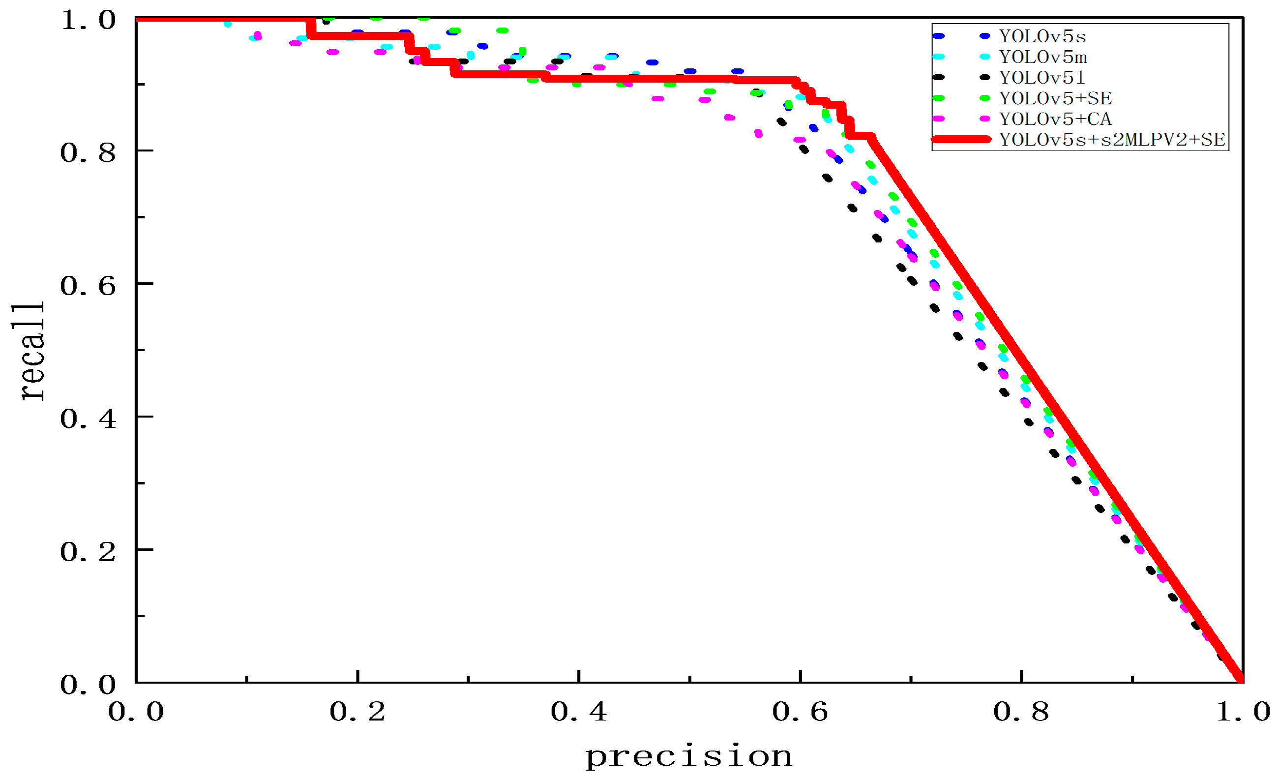
To demonstrate the effectiveness of the proposed enhanced pipeline recognition method, this paper trained six models presented in Table 2 with an identical dataset. The PR curves in Figure 5 illustrate the relationship between the accuracy rate and recall rate, indicating the model’s generalization ability. The PR curve and axes area for YOLOv5s+S2-MLPv2+SE are larger than the other five YOLOv5 models. The results indicate that this enhanced model achieves the best overall performance, with higher average precision and mean average precision metrics than the other models. The trained model was employed to recognize 100 actual SBP submarine pipeline images and the detection results are presented in Table 3.
Table 3 shows that the YOLOv5s base model, when enhanced with the S2-MLPv2 and SE modules and subjected to the SAHI detection, attains a precision of 82.5% and a recall of 99.2%. This indicates a 41.6% improvement in recall compared to the YOLOv5s model. The F1 score is 90.0%, reflecting a 20.2% improvement over the YOLOv5s model. The high recall rate of 99.2% indicates that the enhanced model can accurately identify the most pipelines in actual data. Applying the model to recognize original SBP data significantly reduces manual identification time and enhances detection efficiency in practical production.
In addition, the results show that the YOLOv5s+S2-MLPv2+SE model exhibits significant advantages over other models in terms of R and the F1 score, with a reduced precision. This observation can be attributed to numerous factors affecting the imaging of pipeline targets in real-world data, resulting in a substantial gap between actual and ideal imaging results. Accurately predicting the shape of the pipeline is challenging, leading to a reduction in pipeline identification accuracy.
The key factors influencing pipeline mapping can be summarized as follows:
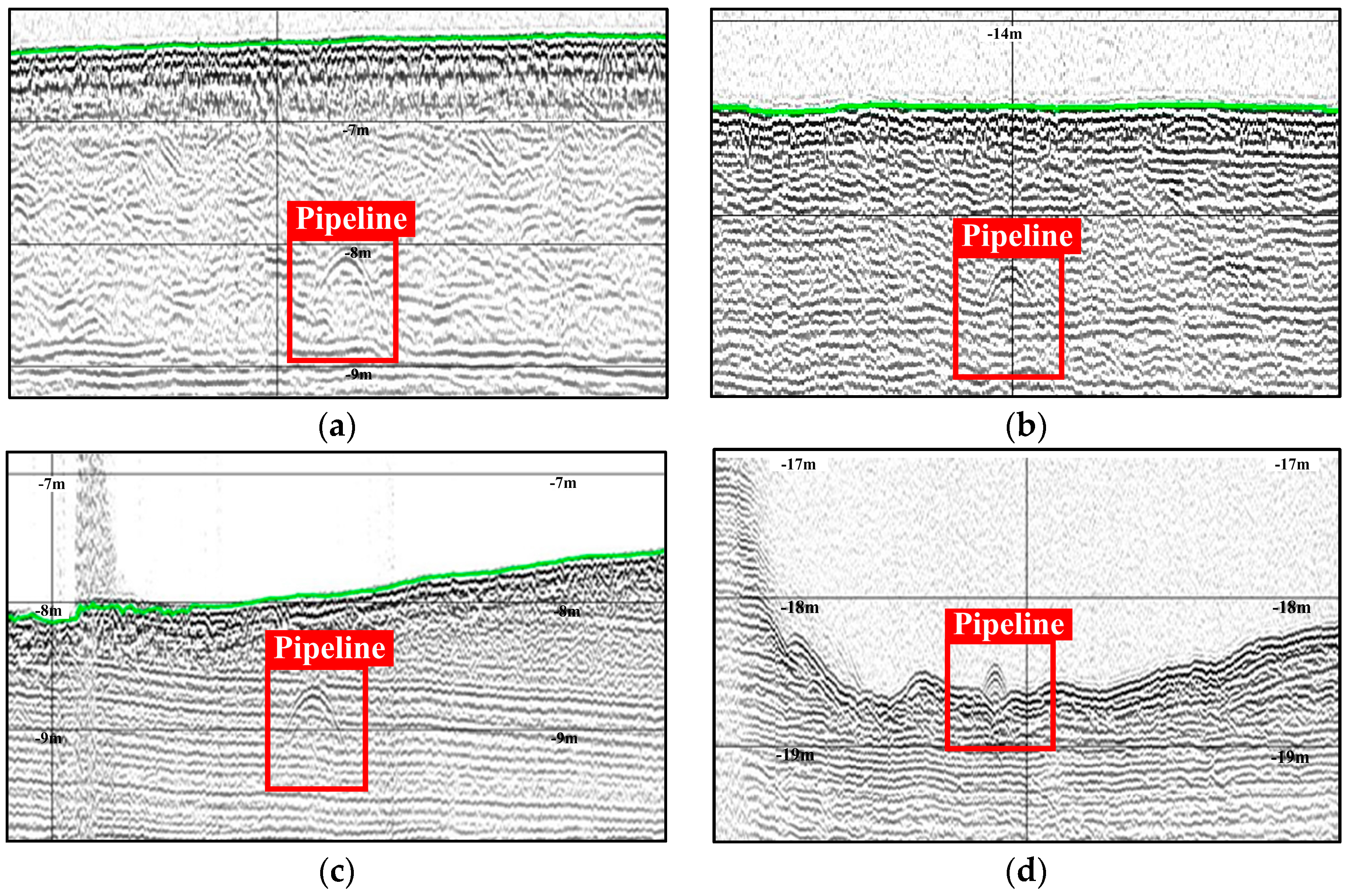
  • Noise impact: Within the bandwidth constraints of the system, extraneous acoustic signals can introduce interference into the sonar-generated image. When a pipeline is positioned near the water surface, the sonar effective beam aperture narrows, and hence reduces the apparent scale of the pipeline within the imagery. This situation presents challenges in differentiating the pipeline from other reflecting objects. Figure 6a.
  • Substrate influence: Different depths and substrates require different detection frequencies. Hard seabeds such as sand, rock, coral reefs, and shells severely limit the depth of acoustic penetration. This restriction hinders the instrument exploration depth, preventing the SBP from effectively receiving echo signals. Figure 6b depicts the impact of a substrate influence on pipeline mapping.
  • Ship swing: During measurement operations, fluctuations in the ship velocity and heading can lead to vessel oscillations. This motion has an effect on the distance between the survey equipment and the pipeline, resulting in distortions to the representation of the pipeline shape within the captured image. Figure 6c shows distortions in pipeline shape caused by ship swing.
  • Air bubble effect: When a considerable volume of air bubbles encircles the transducer within the water medium, the vibrational wave generated through the transducer fails to transmit efficiently into the water as an acoustic pulse. This causes the loss of the pipeline image information such that the SPB will not effectively receive echo signals. Figure 6d shows the loss of the pipeline image information caused by air bubble effect.
The proposed model predicted the best results in practical detection for pipes at different depths, including bare leakage pipelines. Figure 7 presents the specific pipeline detection images.

4. Conclusions

The present study proposes an automated detection method for submarine pipelines using a deep learning model. The approach enhances the feature extraction capability by incorporating the S2-MLPv2 and SE attention modules into the YOLOv5s model. The introduction of the SAHI module addresses challenges associated with detecting small targets in large-sized, low-resolution images with inconspicuous features. This method ensures the effective recognition of SBP pipeline images, eliminating the low efficiency associated with manual identification in traditional submarine pipelines. It efficiently performs automatic identification, assessment, and localization of exposed submarine pipelines, ensuring both efficiency and accuracy in detection. Compared to traditional submarine pipeline methods, significant savings in terms of labor, economic resources and time can be achieved. The improved network model is tested on actual SBP submarine pipeline data collected in Xiangshui County and Dafeng District, Jiangsu Province, China. Experimental results demonstrate that the YOLOv5s+S2-MLPv2+SE model improves recall on the training set by 21.3%, reaching 65.1%, and mAP by 7.9%, reaching 76.0%, compared to the original YOLOv5s benchmark model. On the actual SBP dataset, the recall is enhanced by 41.6%, reaching 99.2%, and the F1 score is improved by 20.2%, reaching 90.0%, in comparison to the base model YOLOv5. The model demonstrates robust identification capabilities for pipes with different buried depths and bare leakage pipes, indicating strong generalization capability. The experimental results show that the improved YOLOv5 model meets the requirements for SBP data pipeline detection. The proposed model demonstrates robustness and a generalization capability, outperforming other target detection algorithms in terms of recall rate and harmonic mean. In addition, there is room for improvement in the accuracy of the model in detecting pipelines. In this experiment, the precision of the enhanced model is 6% lower than that of its baseline model in detecting pipes using real data. There are two main reasons for this; one is that the precision and recall of the model are usually inversely proportional to each other in the data, which results in the phenomenon of higher recall and lower precision. Secondly, because the factors affecting the imaging of pipeline targets in the actual data are noise impact, substrate impact, hull swing and bubble impact, these factors will eventually lead to a large gap between the actual imaging results; the ideal results have difficulty in accurately predicting the shape of the pipeline, which will result in a reduction in the pipeline identification precision. In summary, since the experiments in this paper were conducted in the sea with small topographic undulations, future research work will be conducted in the area of model accuracy improvement and in the sea with large topographic undulations, so as to further verify the robustness and applicability of the model.

Author Contributions

Conceptualization, B.D., S.W., Z.C. and C.L.; methodology, B.D.; software, B.D.; validation, Z.C.; formal analysis, B.D.; investigation, B.D.; resources, S.W.; data curation, S.W. and Z.C.; writing—original draft preparation, B.D.; writing—review and editing, B.D., S.W. and Z.C.; supervision, S.W. and Z.C.; funding acquisition, S.W. and Z.C. All authors have read and agreed to the published version of the manuscript.

Funding

This research was funded by the National Natural Science Foundation of China (42266006), the Jiangxi Provincial7 Natural Science Foundation (20232BAB204089, 20202ACBL214019), and the East China University of Technology Graduate Innovation Fund Project (DHYC-202328).

Institutional Review Board Statement

Not applicable.

Informed Consent Statement

Not applicable.

Data Availability Statement

Due to data security restrictions, the datasets presented in this article are not readily available.

Conflicts of Interest

The authors declare no conflict of interest.

References

  1. Healey, A.J.; Seo, Y.G.T. Dynamic Motions of Marine Pipelines on the Ocean Bottom. J. Energy Resour. Technol. 1984, 106, 65–69. [Google Scholar] [CrossRef]
  2. Wang, K.; Jin, W. The Application Of Acoustic Detection Technology In The Investigation Of Submarine Pipelines. J. Appl. Sci. Process Eng. 2023, 27, 2911–2921. [Google Scholar] [CrossRef]
  3. Gao, L.; Gu, H.-T.; Feng, L. Research on Submarine Buried Oil and Gas Pipeline Autonomous Inspection System of USV. In Proceedings of the ISOPE International Ocean and Polar Engineering Conference, Honolulu, HI, USA, 16 June 2019. [Google Scholar]
  4. Kumudham, R.; Lakshmi, S.; Rajendran, V. Detection of Pipeline Using Machine Learning Algorithm and Analysing the Effect of Resolution Enhancement on Object Recognition Accuracy. J. Xidian Univ. 2020, 14, 1026–1037. [Google Scholar] [CrossRef]
  5. Byrne, B.W. Book Review: Offshore Geotechnical Engineering: Principles and Practice. Géotechnique 2011, 61, 1093. [Google Scholar] [CrossRef]
  6. Baker, J.H.A. Alternative Approaches to Pipeline Survey: The Pipeline Engineer’s View. In SUT Subtech; Springer: Dordrecht, The Netherlands, 1991. [Google Scholar] [CrossRef]
  7. Kaiser, M.J. A Review of Deepwater Pipeline Construction in the U.S. Gulf of Mexico–Contracts, Cost, and Installation Methods. J. Marine. Sci. Appl. 2016, 15, 288–306. [Google Scholar] [CrossRef]
  8. Lurton, X. An Introduction to Underwater Acoustics: Principles and Applications; Springer: Berlin/Heidelberg, Germany, 2003; Volume 84, p. 265. [Google Scholar] [CrossRef]
  9. Jacobi, M.; Karimanzira, D. Multi Sensor Underwater Pipeline Tracking with AUVs. In Proceedings of the 2014 Oceans—St. John’s, St. John’s, NL, Canada, 14–19 September 2014; pp. 1–6. [Google Scholar] [CrossRef]
  10. Lv, Y.; Dong, Y.; Li, Y.; Wu, H.; Hu, K.; Hu, H.; Feng, W. Submarine Cable Fault Identification Based on FCN-GRU-SVM. E3S Web Conf. 2022, 360, 01055. [Google Scholar] [CrossRef]
  11. Bharti, V.; Lane, D.; Wang, S. A Semi-Heuristic Approach for Tracking Buried Subsea Pipelines Using Fluxgate Magnetometers. In Proceedings of the 2020 IEEE 16th International Conference on Automation Science and Engineering (CASE), Hong Kong, 20–21 August 2020; pp. 469–475. [Google Scholar] [CrossRef]
  12. Li, S.; Zhao, J.; Zhang, H.; Zhang, Y. Automatic Detection of Pipelines from Sub-Bottom Profiler Sonar Images. IEEE J. Oceanic Eng. 2022, 47, 417–432. [Google Scholar] [CrossRef]
  13. Guan, M.; Cheng, Y.; Li, Q.; Wang, C.; Fang, X.; Yu, J. An Effective Method for Submarine Buried Pipeline Detection via Multi-Sensor Data Fusion. IEEE Access 2019, 7, 125300–125309. [Google Scholar] [CrossRef]
  14. Wunderlich, J.; Wendt, G.; Müller, S. High-Resolution Echo-Sounding and Detection of Embedded Archaeological Objects with Nonlinear Sub-Bottom Profilers. Mar. Geophys. Res. 2005, 26, 123–133. [Google Scholar] [CrossRef]
  15. Wang, C.; Jiang, Y.; Wang, K.; Wei, F. A Field-Programmable Gate Array System for Sonar Image Recognition Based on Convolutional Neural Network. Proc. Inst. Mech. Eng. Part I J. Syst. Control. Eng. 2021, 235, 1808–1818. [Google Scholar] [CrossRef]
  16. Zheng, G.; Zhang, H.; Li, Y.; Zhao, J. A Universal Automatic Bottom Tracking Method of Side Scan Sonar Data Based on Semantic Segmentation. Remote Sens. 2021, 13, 1945. [Google Scholar] [CrossRef]
  17. Li, J.; Chen, L.; Shen, J.; Xiao, X.; Liu, X.; Sun, X.; Wang, X.; Li, D. Improved Neural Network with Spatial Pyramid Pooling and Online Datasets Preprocessing for Underwater Target Detection Based on Side Scan Sonar Imagery. Remote Sens. 2023, 15, 440. [Google Scholar] [CrossRef]
  18. Chen, Z.; Wu, R.; Lin, Y.; Li, C.; Chen, S.; Yuan, Z.; Chen, S.; Zou, X. Plant Disease Recognition Model Based on Improved YOLOv5. Agronomy 2022, 12, 365. [Google Scholar] [CrossRef]
  19. Yang, L.; Yuan, G.; Zhou, H.; Liu, H.; Chen, J.; Wu, H. RS-YOLOX: A High-Precision Detector for Object Detection in Satellite Remote Sensing Images. Appl. Sci. 2022, 12, 8707. [Google Scholar] [CrossRef]
  20. Keles, M.C.; Salmanoglu, B.; Guzel, M.S.; Gursoy, B.; Bostanci, G.E. Evaluation of YOLO Models with Sliced Inference for Small Object Detection. arXiv 2022, arXiv:2203.04799. [Google Scholar] [CrossRef]
  21. Jocher, G. YOLOv5 by Ultralytics 2020. Available online: https://github.com/ultralytics/yolov5 (accessed on 1 March 2024).
  22. Hou, Q.; Zhou, D.; Feng, J. Coordinate Attention for Efficient Mobile Network Design. In Proceedings of the 2021 IEEE/CVF Conference on Computer Vision and Pattern Recognition (CVPR), Nashville, TN, USA, 20–25 June 2021; pp. 13708–13717. [Google Scholar] [CrossRef]
  23. Weston, J.; Sukhbaatar, S. System 2 Attention (Is Something You Might Need Too). arXiv 2023, arXiv:2311.11829. [Google Scholar] [CrossRef]
  24. Hu, J.; Shen, L.; Sun, G. Squeeze-and-Excitation Networks. In Proceedings of the IEEE Conference on Computer Vision and Pattern Recognition, Salt Lake City, UT, USA, 18–23 June 2018; pp. 7132–7141. [Google Scholar] [CrossRef]
  25. Akyon, F.C.; Altinuc, S.O.; Temizel, A. Slicing Aided Hyper Inference and Fine-Tuning for Small Object Detection. In Proceedings of the 2022 IEEE International Conference on Image Processing (ICIP), Bordeaux, France, 16–19 October 2022; pp. 966–970. [Google Scholar] [CrossRef]
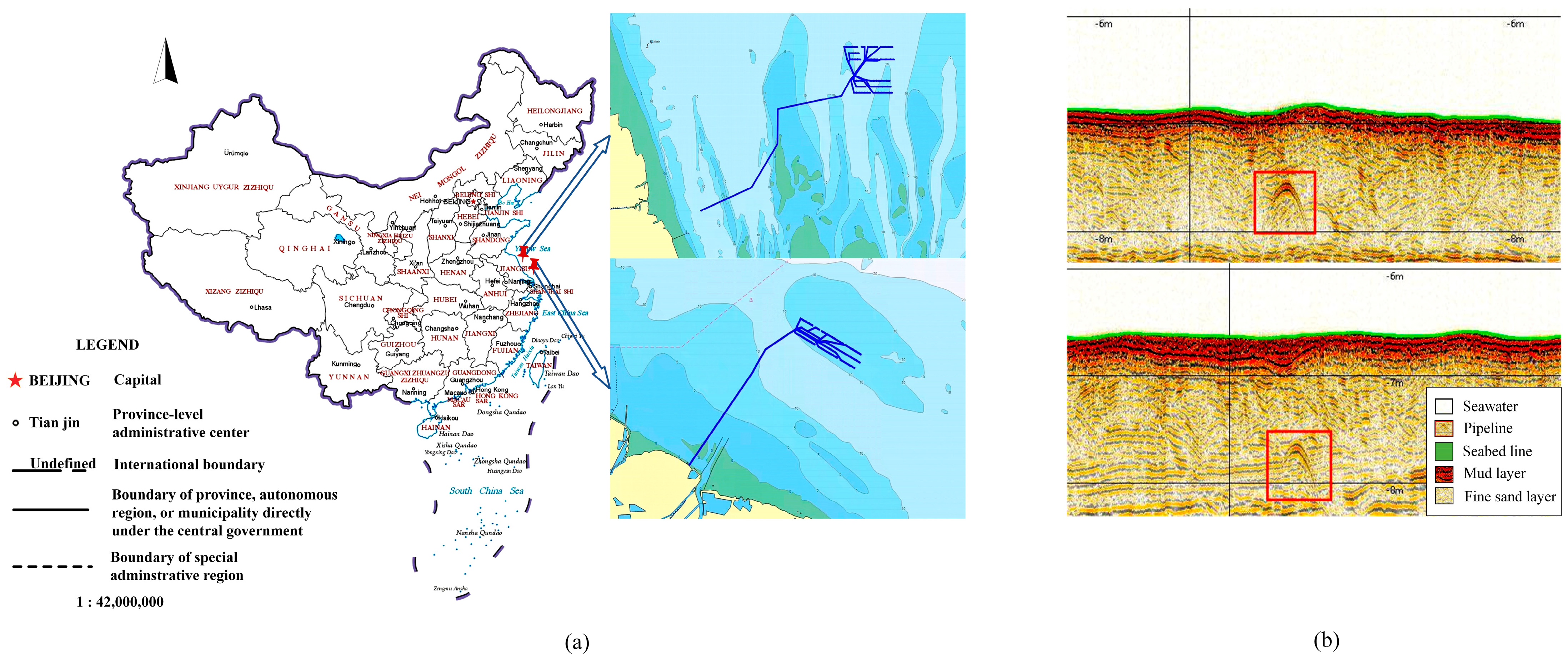
Figure 1. (a) Research area. (b) Sub-bottom stratigraphic map of the study area. The blue solid line in figure (a) indicates the track route of the collected data, and the one in the red box in figure (b) indicates the submarine pipeline.
Jmse 12 00451 g001
Figure 2. Flowchart of the proposed method.
Jmse 12 00451 g002
Figure 3. YOLOv5 network architecture with added attention mechanism.
Jmse 12 00451 g003
Figure 4. Detection process flowchart after incorporating the SAHI model.
Jmse 12 00451 g004
Figure 5. Experimental model PR curve graph.
Jmse 12 00451 g005
Figure 6. Graphs of the SBP produced by different influential factors (ad). The figures show measured pipeline images under various adverse conditions.
Jmse 12 00451 g006
Figure 7. Pipeline recognition effect diagram. (a) A pipeline detection diagram at buried depths of 1-1.5 m. (b) A pipeline detection diagram for buried depths greater than 1.5 m. (c) A pipeline detection diagram for buried depths less than 1 m. (d) An exposed pipeline detection diagram.
Jmse 12 00451 g007
Table 1. Other variables configuration for model execution.
ParameterConfiguration
Operating systemWindows 11
Deep learning frameworkPyTorch 1.9.1+cu111
Programming languagepython3.9
GPU accelerated environmentcuda11.1
GPUNVIDIA GeForce RTX 4060 Laptop
CPU12th Gen Intel(R) Core(TM) i7-12650H
Table 2. Table of Experimental Data Precision for Different Models.
ModelsPR[email protected]
YOLOv5s0.8520.4380.681
YOLOv5m0.8610.6100.749
YOLOv5l0.8400.5550.729
YOLOv5s+SE0.8450.6370.754
YOLOv5s+CA0.8120.6230.727
YOLOv5s+S2-MLPv2+SE0.8480.6510.760
Table 3. Accuracy SBP Submarine Pipeline Identification.
ModelsPRF1
YOLOv5s0.8850.5760.698
YOLOv5m0.7960.8720.832
YOLOv5l0.8700.8560.863
YOLOv5s+SE0.8080.8400.823
YOLOv5s+CA0.8240.8720.818
YOLOv5s+S2-MLPv2+SE0.8250.9920.900
Disclaimer/Publisher’s Note: The statements, opinions and data contained in all publications are solely those of the individual author(s) and contributor(s) and not of MDPI and/or the editor(s). MDPI and/or the editor(s) disclaim responsibility for any injury to people or property resulting from any ideas, methods, instructions or products referred to in the content.