1. Introduction
Computer-based approaches are progressively employed to estimate air quality and predict alterations in pollution levels. Air pollution has been established as a significant contributor to numerous health issues, leading to premature deaths [
1,
2]. Authors in [
3] demonstrated the negative effects of PM
10 pollutants on human health, and [
4] studied the health effects of particulate ambient air pollution exposure and elucidated the association between air pollution and cardiovascular disease. Diverse pollution models are presently in use throughout Europe. The focus of this research is the maritime area of the Bay of Algeciras, which contains a powerful and large chemical pole, the Gibraltar airport, which currently has a high flow of flights, and above all, the Algeciras port receiving thousands of vessels and trucks per year, and multiple roads full of private traffic. In recent years, different studies have been carried out in different countries using advanced statistical techniques and machine learning [
5,
6,
7,
8,
9]. This research aims to use a mixture of techniques: air pollution forecasting together with graphical methods. In the study area of pollution, namely in marine pollution, new applications in the field of graphical research have been studied [
10]. The geospatial analysis of pollution provides valuable insights into environmental changes and urban development. For this reason, geospatial modelling has been used in numerous fields including endangered species monitoring [
11]. An increasing demand exists for the application of geospatial artificial intelligence analysis to diverse environmental datasets in order to derive solutions that positively impact frontline communities. One such crucially needed solution involves predicting ambient ground-level air pollution concentrations, which are pertinent to public health. However, numerous challenges are associated with this endeavour, including the limited size and representativeness of ground reference stations for model development, the integration of data from multiple sources, and the interpretability of machine learning models. This research endeavours to address these challenges by utilising a strategically deployed and extensive network of low-cost sensors (LCS), which have undergone rigorous calibration through an optimised neural network approach [
12,
13,
14].
Many scientific papers have produced air pollution maps, including works by [
15,
16,
17,
18,
19,
20,
21]. While in a distinct field, the research by [
18] aims to accurately generate spatial interpolation patterns of combustion product concentrations, employing mapping techniques with ArcGIS and providing valuable information. In this research domain, various studies involving pollution mapping have been conducted. In [
19], an artificial neural network ensemble is proposed to estimate hourly NO
2 concentration maps, giving slightly better results than Inverse Distance Weighted (IDW) and kriging. Understanding that monitoring air quality in cities enhances the well-being of citizens, cyclists, and pedestrians is crucial. Therefore, ref. [
20] introduced a real-time monitoring method that utilises atmospheric maps, enabling individuals to choose the least polluted route. In the University of North Texas, as described in [
21], PM
2.5 particle monitoring is conducted using a dynamic bicycle equipped with a GPS system. Concentrations of this pollutant are then estimated and mapped. Numerous studies discuss the use of wireless sensors [
20,
22] for monitoring air quality, which is subsequently leveraged to predict pollutant concentrations and display them on maps [
22]. In [
23], publicly available TROPOMI-S5 satellite data are employed, compared with measurements obtained from ground stations in Poland. The approach proposed by [
24] aims to develop a method for deriving particulate matter (PM) emissions maps from in situ PM concentration measurements using an inverse model generating air pollution maps. The study by [
25] indicates that mobile sensors can improve the spatio-temporal resolution of the received pollution data but, nevertheless, the quality of the mobile sensors is important in order to be reliable. These mobile sensors are used in the study from [
26], where it is shown that by deploying low-cost wireless sensors, it is possible to obtain more accurate and real-time air pollution levels at different locations. Sensors installed on public transport vehicles complement the readings from stationary sensors. The study’s objective is to evaluate pollutant concentrations and establish a spatiotemporal pattern of changes in Central and Eastern Europe, specifically in Poland and Ukraine. The importance of reducing the waiting times of ships in ports in order to reduce the pollution associated with them is discussed in [
27]. The authors in [
28] proposed the raster datasets, generated through land use regression models derived from the European Study of Cohorts for Air Pollution Effects (ESCAPE) project. The need for interpolating irregularly spaced empirical areal data, representing diverse locations such as weather observation stations, surveyed sites, data-collection zones, or observation locations, is prevalent in various fields. As exposed in [
29], this interpolation is crucial for generating a continuous surface, facilitating the comparison and analysis of data points. Defining a continuous function that precisely fits the given values is essential to achieve this. This function allows for the creation of contour maps, perspective views, and the evaluation of interpolated information.
This work is framed in a similar line to the aforementioned studies. Previous work has focused on the prediction of air pollution using machine learning and meteorological data such as in [
30,
31,
32], highlighting the latest studies based on deep learning techniques in [
30,
31]. In [
31], the study focuses on predicting maritime traffic-related pollutant concentrations in the Bay of Algeciras, Spain. Using data from 2017 to 2019, various models, including artificial neural networks, were tested and compared for accuracy. The best models showed high sensitivities, indicating their potential for forecasting air pollution in port cities and aiding decision making for pollution prevention. The research by [
32] focuses on air quality prediction in the industrially intense Bay of Algeciras, Spain, from 2017 to 2019. The study serves as a valuable resource for informed decision making by authorities, companies, and citizens due to its relevance in predicting air quality in a highly industrialised area. By integrating data visualisation tools and digital mapping techniques, the research findings have been transformed into visual maps. These maps provide a comprehensive geospatial representation of pollutant concentrations across different zones in the region, enabling a holistic understanding of distribution patterns and identification of areas with elevated pollution levels.
This new article seeks to generate predictions across various forecasting timelines and present them graphically.
Section 2 includes the Materials and Methods,
Section 3 is the Results,
Section 4 presents the Discussion, and, finally,
Section 5 discusses the main conclusions.
2. Materials and Methods
2.1. Materials
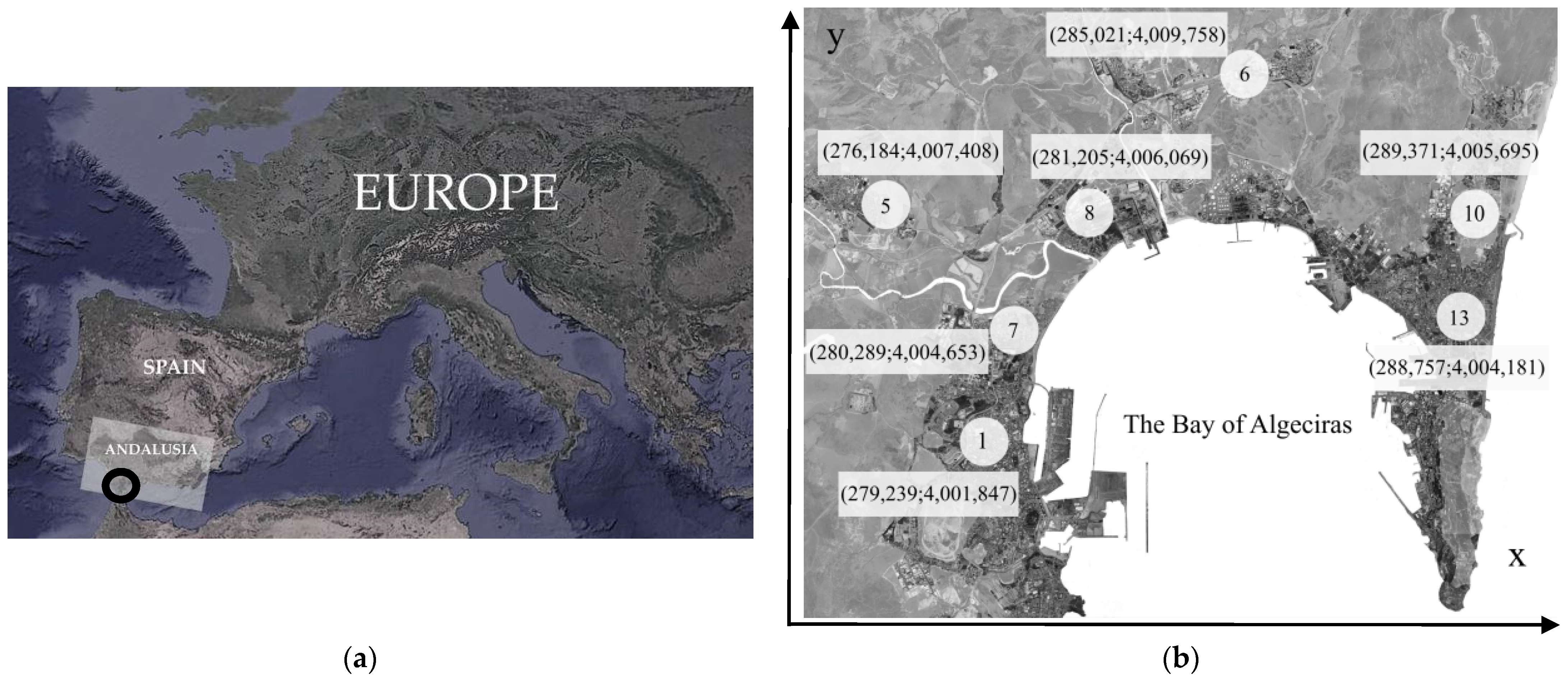
As part of a continuous endeavour to comprehend and tackle contemporary environmental issues, an exhaustive investigation was undertaken to observe levels of pollutants at various sites within the Bay of Algeciras region. The sensorised area of The Bay of Algeciras (in the South of Spain,
Figure 1a) is a highly polluted zone where industries, an airport, and a huge port coexist. This complex scenario is explained in more detail:
Industrial Activities: The Campo de Gibraltar region is heavily industrialised, with oil refineries, chemical plants, and industrial ports releasing significant PM pollution, contributing 30% to 50% or more.
Transportation: Road traffic, shipping, and other transport activities, especially diesel vehicles, are major PM sources. The Port of Algeciras may contribute 20% to 40% of PM pollution.
Natural Sources: Natural sources like wind-blown dust from the Sahara Desert, sea spray, and wildfires play a smaller role, typically contributing 5% to 15% of PM pollution.
In Andalusia, managed by Conserjería de Medio Ambiente, a variety of sensors are used for monitoring PM10 in the air quality monitoring and control network. These sensors typically include a combination of the following:
- -
Particle filters (gravimetric or impact): These sensors capture airborne particles on a filter over a specific period of time. The filters are then weighed to determine the concentration of PM10 particles.
- -
Optical analysers: These sensors use light scattering to measure the concentration of particles in the air.
- -
Impact sensors: These sensors use impact techniques to collect particles on a substrate and then measure the concentration of captured particles.
- -
Beta attenuation sensors: These sensors use the attenuation of a beta particle beam to measure the concentration of suspended particles in the air.
The sensors used in this work provide data validated by a public institution such as the Andalusian Regional Government in Spain. They do not exhibit errors in calibration precision or drift, but they may encounter errors due to random fluctuations caused by sensor electronics, environmental conditions, external factors, or the inherent nature of the sensor.
In this work, a three-year period of data on PM
10 pollutants, from 2017 to 2019, has been analysed. Seven particulate matter sensors (described in
Figure 1b and
Table 1) record this pollutant concentrations (µg/m
3) in several cities of the Bay. Andalusian authorities collected intricate PM
10 pollution data in the maritime environment of the Bay of Algeciras, which was graciously shared with the University of Cádiz.
The aim is to create a virtual network of pollution maps showing the predicted evolution of the concentrations of this pollutant at each sensor (or city). The UTM coordinates of each of the available monitoring stations in the Bay of Algeciras measuring PM
10, as described in
Table 1, were required, and they have been taken from the official website of the Andalusian air quality monitoring and control network.
The first step is database preprocessing, which involves the imputation of missing data using the available information using ANNs, modelling each station as a function of the rest of the stations. A percentage of less than 3% of gaps have been filled in La Línea station (which is the station with more gaps). In addition, a standardisation of the concentration of PM10 pollutants and outliers elimination has been developed using the method based on the standard deviation (σ) to the mean value. Any data point that falls outside the range ( 3·σ) is detected as an outlier. In this work, some peaks have been left in the database after a visual inspection.
The gathering of this information has not only enabled a comprehensive examination of past pollution patterns but has also established the foundation for a proactive strategy to anticipate forthcoming pollution levels in the area. Employing statistical modelling and machine learning methodologies, a precise predictive framework has been formulated, foreseeing potential pollution scenarios over a specified period.
The current study employs a two-stage methodology. Initially, a future forecast of pollutant concentrations is conducted at each monitoring station within the designated study area. Subsequently, leveraging the localised predictions, a geostatistical interpolation is executed using the Inverse Distance Weighting (IDW) algorithm, yielding concentration values for each () coordinate pair and facilitating the creation of a concentration prediction map.
In the first stage, the prediction is carried out by selecting the optimal model from various configurations. This selection is achieved through a cross-validation procedure and a multiple-model comparison procedure, employing the Friedman and Bonferroni methods. Once the most suitable model is identified, predictions are made at each station.
In data analysis, the crucial aspects to evaluate in a model revolve around its generalisation capabilities, which gauge its performance in real-world scenarios. This entails assessing how well a model operates when applied to authentic examples that were not utilised during its initial design. Therefore, the training and test stages are fundamental components of building and evaluating predictive models. The first step involves selecting a representative dataset that includes both input features (independent variables) and the corresponding output or target variable (dependent variable). This dataset is divided into two subsets: one for training and one for testing. During the training process, the algorithm learns patterns and relationships within the data to make predictions on new, unseen data. Additionally, a parameter tuning is developed. A 2-fold-cross validation (2-CV) is employed during the training and testing process to ensure robustness and reduce the impact of the specific dataset split. Once the model is trained, it must undergo evaluation on an independent dataset it has not encountered before, referred to as the testing dataset. This evaluation assesses the ability of the model to generalise to new, unseen data. The trained model is employed to predict features within the testing dataset, and these predictions are then compared against the actual values in the testing dataset. Various metrics, such as the determination coefficient (R) and mean squared error (MSE) for regression problems, are computed to gauge the performance of the model. Some analyses also incorporate a validation set during the training phase, aiding in decisions about model hyperparameters and preventing overfitting. In addition, we repeat the experiment a certain number of times since the result always depends on the initial random weights. Thus, for each configuration, we can have 20 performance measures, which are then compared with the Friedman test to determine if the means are equal, and if they are not, to determine which is the best model.
The methodology used in this article consists of preparing the database of PM10 concentration data, performing an imputation of missing data, studying outliers, selecting the best model, etc., and using artificial neural networks to predict future values of this pollutant at , and . Two experiments have been carried out for this purpose. The first one consists of making a simple prediction with the hourly databases one hour ahead. The second experiment also uses time jumps, generating an autoregressive matrix to be used as the input of the models ( consecutive previous values and jumps).
2.2. Methods
2.2.1. Shallow Artificial Neural Networks (Shallow ANNs)
Shallow Artificial Neural Networks (Shallow ANNs) used in this research are fully connected feedforward ANNs that can effectively model multi-dimensional mapping problems when provided with consistent data and a sufficient number of neurons in their hidden layer [
33]. They consist of a network of interconnected nodes called “artificial neurons” that are organised in layers (input layer, hidden or intermediate layer(s), and output layer). During training, the neural network is fed with data and adjusts the weights of the connections between the neurons so that the output of the network moves closer and closer to the desired output. The equation expressing a neural network is given by a well-known expression where the weights (
) are different by adjusting for each connection or neuron (see Equation (1)). It follows that the vector of weights
is a dynamic system that minimises the error.
The differential equation (general) performs the function of representing the learning law that is based on the task of finding the weights that allow the desired knowledge to be encoded in the network, in this case, using backpropagation supervised learning. Once this objective has been achieved, the network is ready to respond to new input vectors with coherent outputs, thanks to the generalisation capacity it has acquired. It is important to note that this generalisation capacity must be evaluated in each situation to measure the performance of the system.
In [
33], it was proved that ANNs with at least one hidden layer are universal approximators. Nevertheless, determining the optimal number of neurons required for learning to model the relationship between input and output variables is inherently uncertain. However, it is impossible a priori to know what number of neurons is necessary to learn to model a mapping between predicted values as a function of past values. Therefore, sampling procedures are employed to gather results across various iterations, using predicted values as a function of past values, followed by model comparisons using methods like ANOVA or Friedman’s test, or through the application of Bayesian optimisation procedures.
2.2.2. Inverse Distance Weighting (IDW)
Inverse Distance Weighting (IDW) was proposed for the first time by [
34] and assumes that each measured point has a local influence that decreases with distance. It gives higher weights to points closer to the prediction location and the weights decrease as a function of distance (hence, the name inverse distance weighted). IDW is a method used in spatial interpolation to estimate unknown values at unsampled locations based on observed values at known locations. This is a mathematical (deterministic) method that assumes that nearby values have more influence on the estimate than more distant values. The fundamental idea is to assign weights to known data points based on the inverse of their distance from the prediction location. Closer points have more weight in the estimate than more distant points. The weights (
) are assigned to the known data points, as Equation (2) shows.
where
is the Euclidean distance between the prediction point and the known data point
,
is the parameter that controls the influence of distance on weighting. The value of
≥ 1 may vary depending on the nature of the data and the spatial distribution of the known points. A common value is 2, but other values are also possible. The estimate of the value at an unsampled location (
) is made by weighting the observed values (
) as a function of their inverse distances and summing these weighted products (Equation (3)).
where
is the number of known data points. This technique is used in many manuscripts, such as [
35,
36,
37].
2.3. Experimental Procedure
A resampling technique has been employed to mitigate test set prediction errors and counteract overfitting. Performance results were exclusively gathered for the test set to estimate the generalisation error of each model using unseen data, following a methodology successfully implemented in prior studies [
30,
31]. We implemented a two-fold cross-validation technique to identify the optimal model, considering its generalisation performance. The data is initially partitioned into three separate categories: training, validation, and test sets. The validation set is employed to implement early stopping and prevent overfitting. Following this, we estimate the parameters for each model using one of the groups, specifically the training set. Subsequently, the test set is utilised to evaluate the results, simulating the practical performance of the model. This entire procedure is iterated 20 times, and the outcomes are averaged across these iterations.
Different configurations have been tested using different hidden neurons (1, 2, 5, 10, 20, 30, and 50) in two different experiments:
The first experiment is based on hourly data of PM
10 pollutants using an autoregressive scheme for a 1 h ahead forecasting using
consecutive lags in the past, as Equation (4) shows.
The second experiment is for a 4 h ahead forecasting and is also based on an hourly time series of PM
10 pollutants, but, furthermore, includes an autoregressive scheme using
consecutive lags and
consecutive “jumps” in the past as shown in Equation (5).
where
is the number of sequential lags to be considered ();
is the number of jumps to be considered ().
2.4. Multiple Comparison Methods
Finding the best prediction model at each monitoring station is the objective of this stage. Different ANN topologies are tested within a random resampling procedure where 20 replications were made and MSE and R values allow us to select the best configuration using a statistical multiple comparison procedure.
In this study, we employed the non-parametric variant of the ANOVA test, namely the Friedman test, to assess whether the means of all tested models are equivalent. If equality is observed, we may opt for the simplest model based on Occam’s razor criterion. However, if the means of the model outcomes differ, given that the Friedman method only determines the null hypothesis regarding equal means, we will utilise the Bonferroni method. This approach helps identify significant differences between the models, allowing us to select the most suitable one. Thus, the Bonferroni test is used to determine which is the best model at each location.
4. Discussion
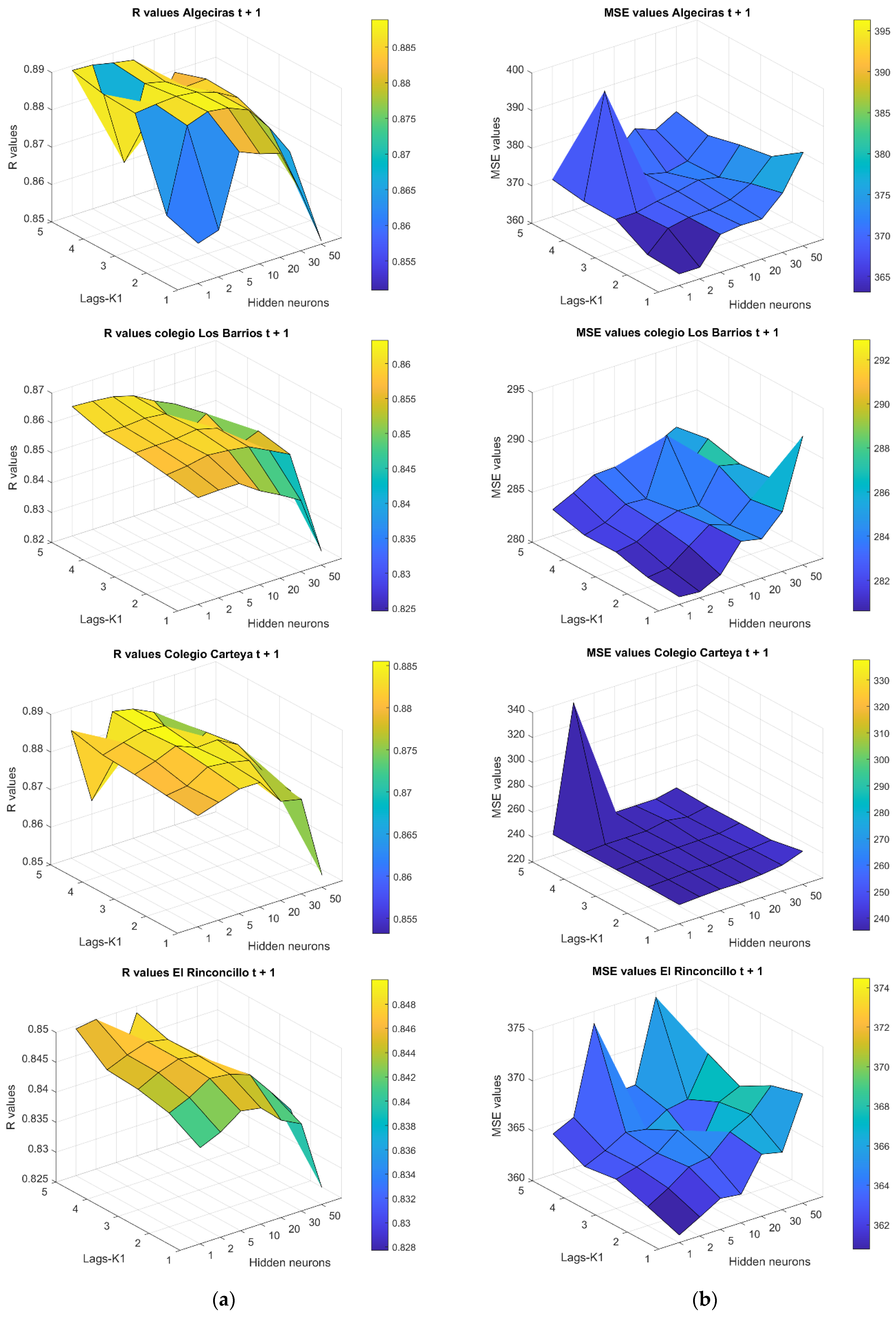
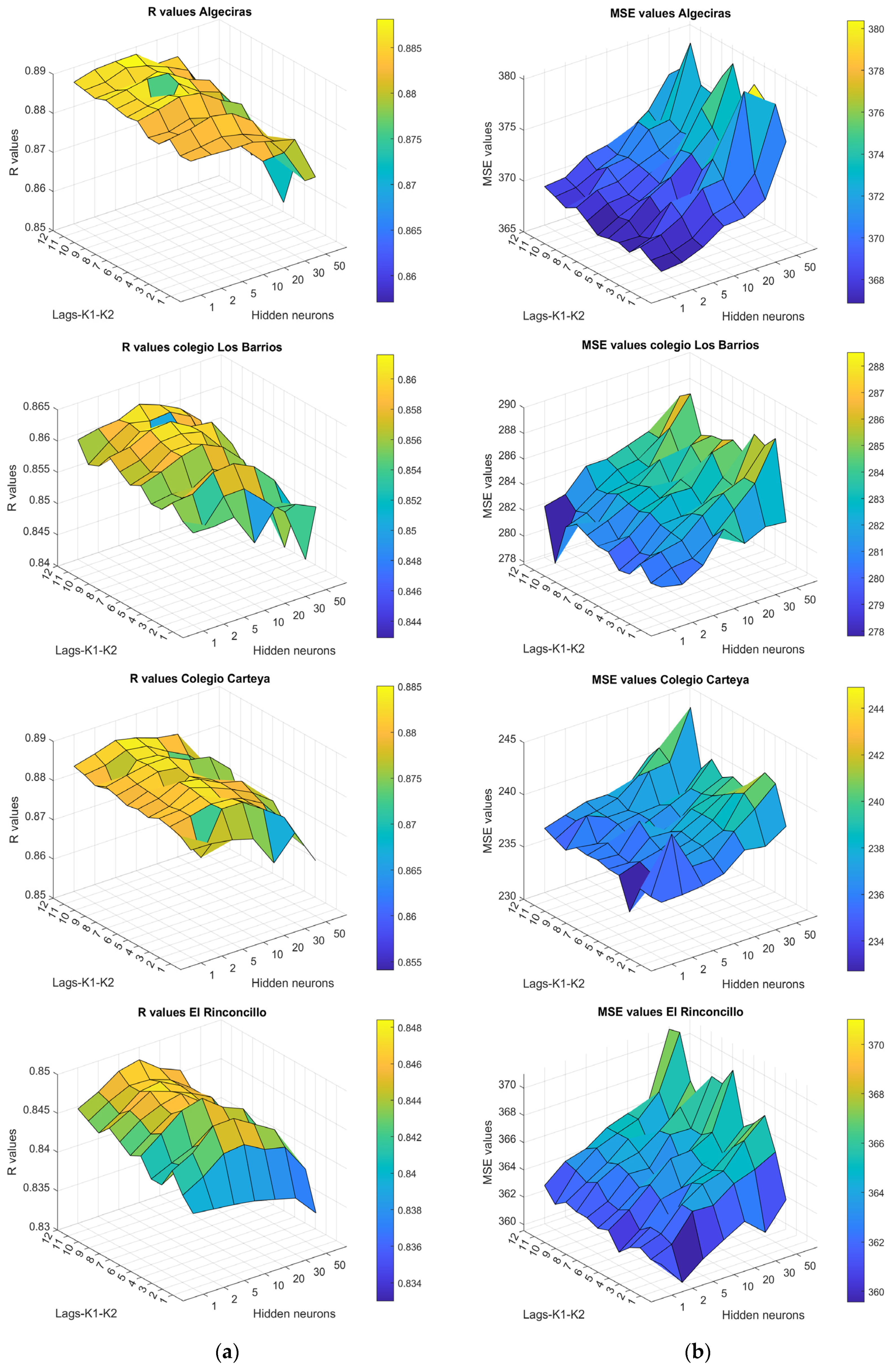
In general, the models perform quite well, with
R values higher than 0.85 in all cases as we can see in scenario 1. The correlation coefficient,
R, experiences little change with the amount of past information. In
Figure 2, the predictions at timestamp
indicate that optimal models tend to exhibit fewer neurons, and a limited depth of historical data is required. For the first station, station 1, Algeciras, the best model, with an
R value of almost 0.89 and an
MSE of 390, consists of 1 hidden neuron and 3 to 5 lags (
or steps backwards). The same number of neurons indicates the best model in Colegio Los Barrios, station 5, with a correlation value,
R, of 0.865 and an error,
MSE, of 290. In the case of Colegio Carteya, station 6, 5 hidden neurons yield the highest
R value, almost 0.89, and the lowest
MSE of 240, making it the best model for lags (
) from 1 to 4. Finally, in the case of El Rinconcillo, station 7, we observe that between 5 and 10 neurons indicate the best model with lags (
) from 1 to 4. The highest
R value in El Rinconcillo is nearly 0.85, with a
MSE of 365.
Likewise, concerning the predictions at timestamp
(scenario 2), it is generally observed that optimal outcomes are achieved by incorporating a specific number of historical data points, lags or steps backwards (
), varying depending on each monitoring station. The impact of past information on the correlation coefficient (
R) varies, leading to fluctuations rather than a consistent trend observed in the case of
. In
Figure 3, predictions at timestamp
(scenario 2) revealed that the optimal models are achieved with fewer hidden neurons. At the Algeciras station, a high
R value of nearly 0.89 and an
MSE of less than 370 are obtained. At Colegio Los Barrios station, the highest
R value reaches up to 0.86 with 10 hidden neurons and an
MSE of 284. Similarly, at Carteya station, the highest
R value is up to 0.88 with an
MSE of up to 235. At El Rinconcillo station, the highest
R value is approximately 0.845 with an
MSE of almost 364. Notably, in stations such as Carteya and El Rinconcillo, the most effective models are identified with an intermediary range of hidden neurons, ranging from 10 to 20. The error
MSE is in almost all models in the same line except for some sharp increase, especially in cases of 50 neurons in the hidden layer.
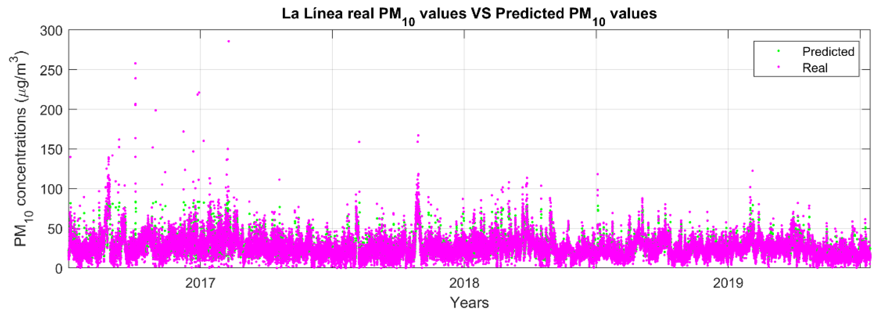
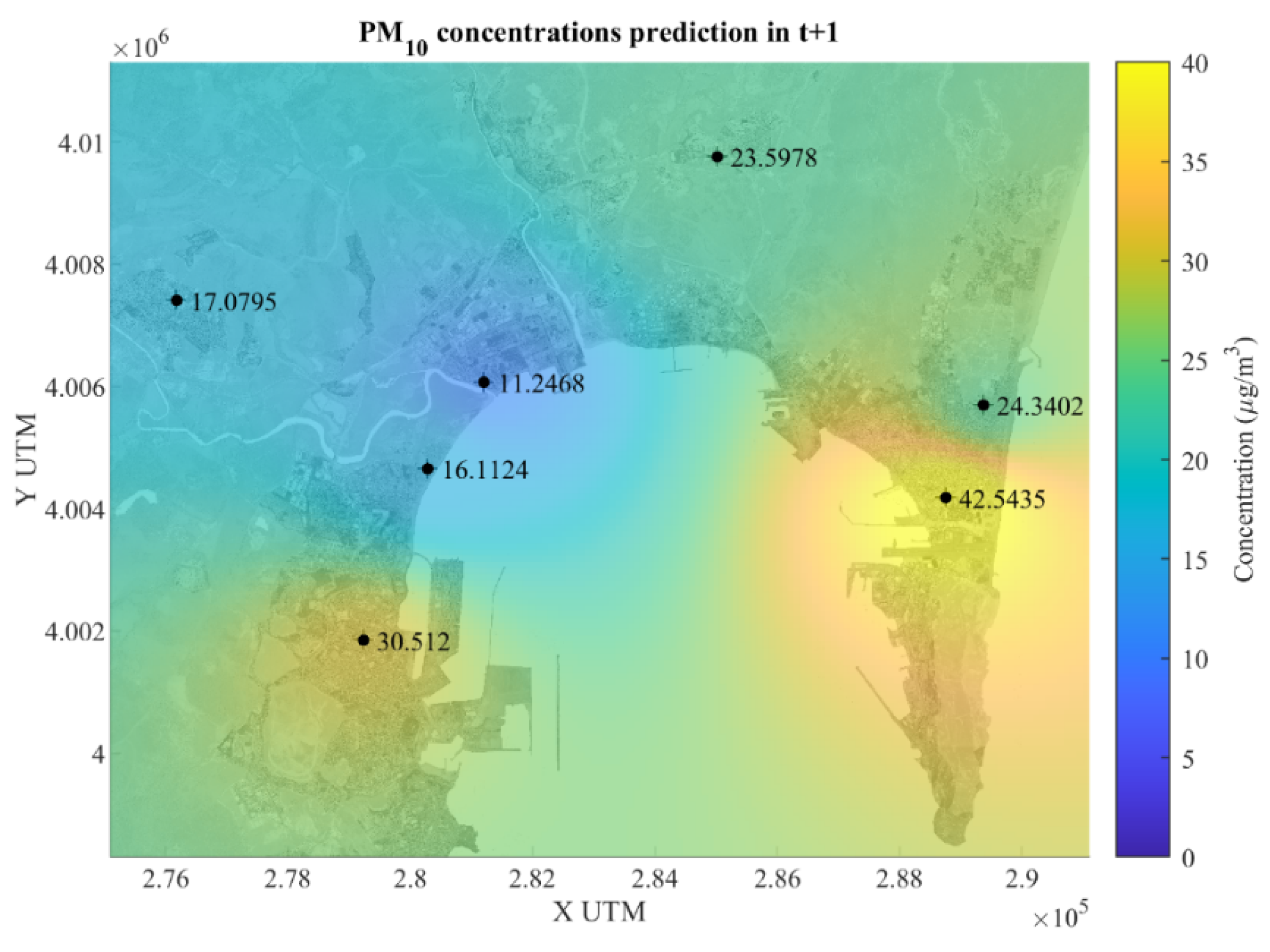
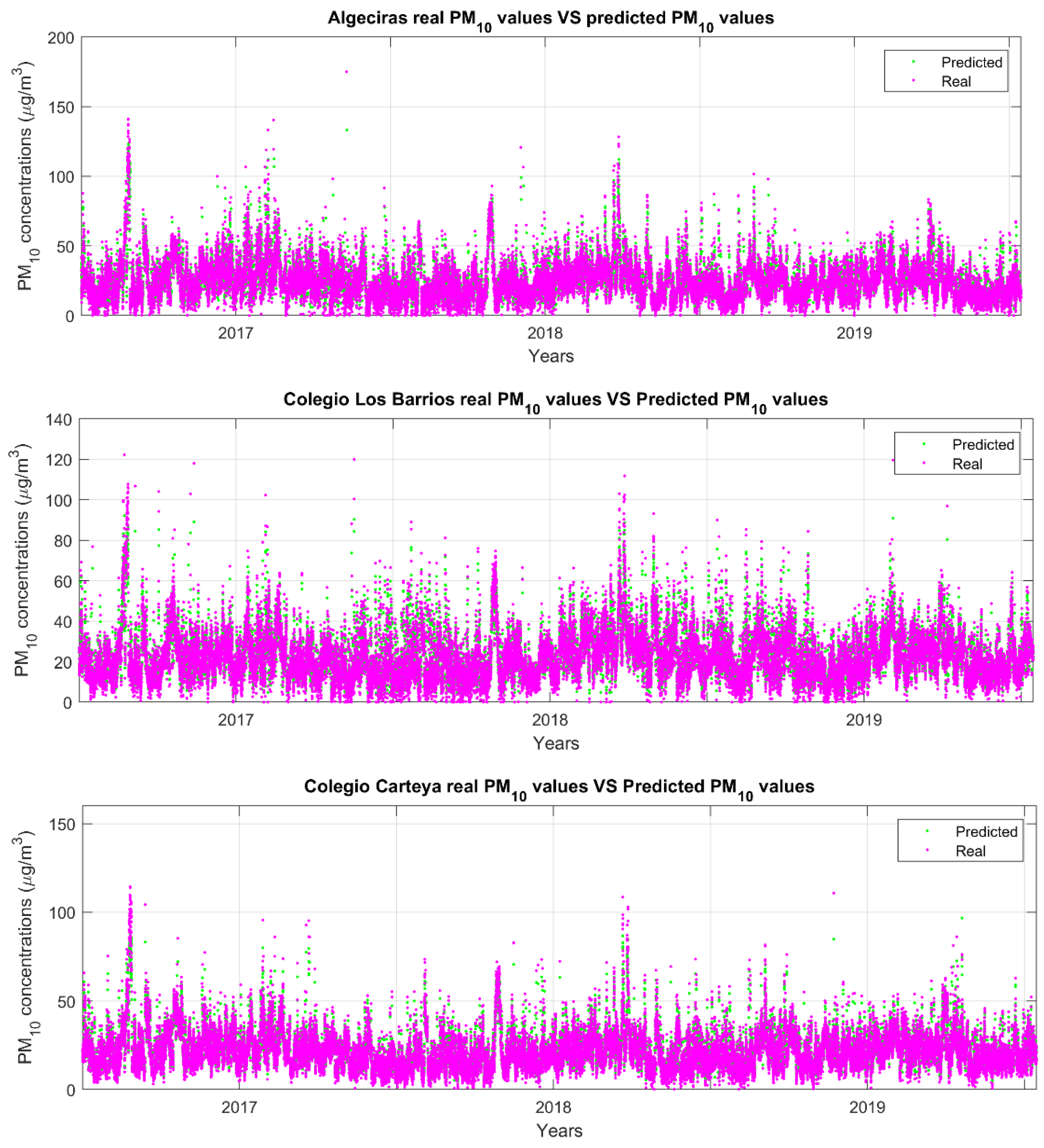
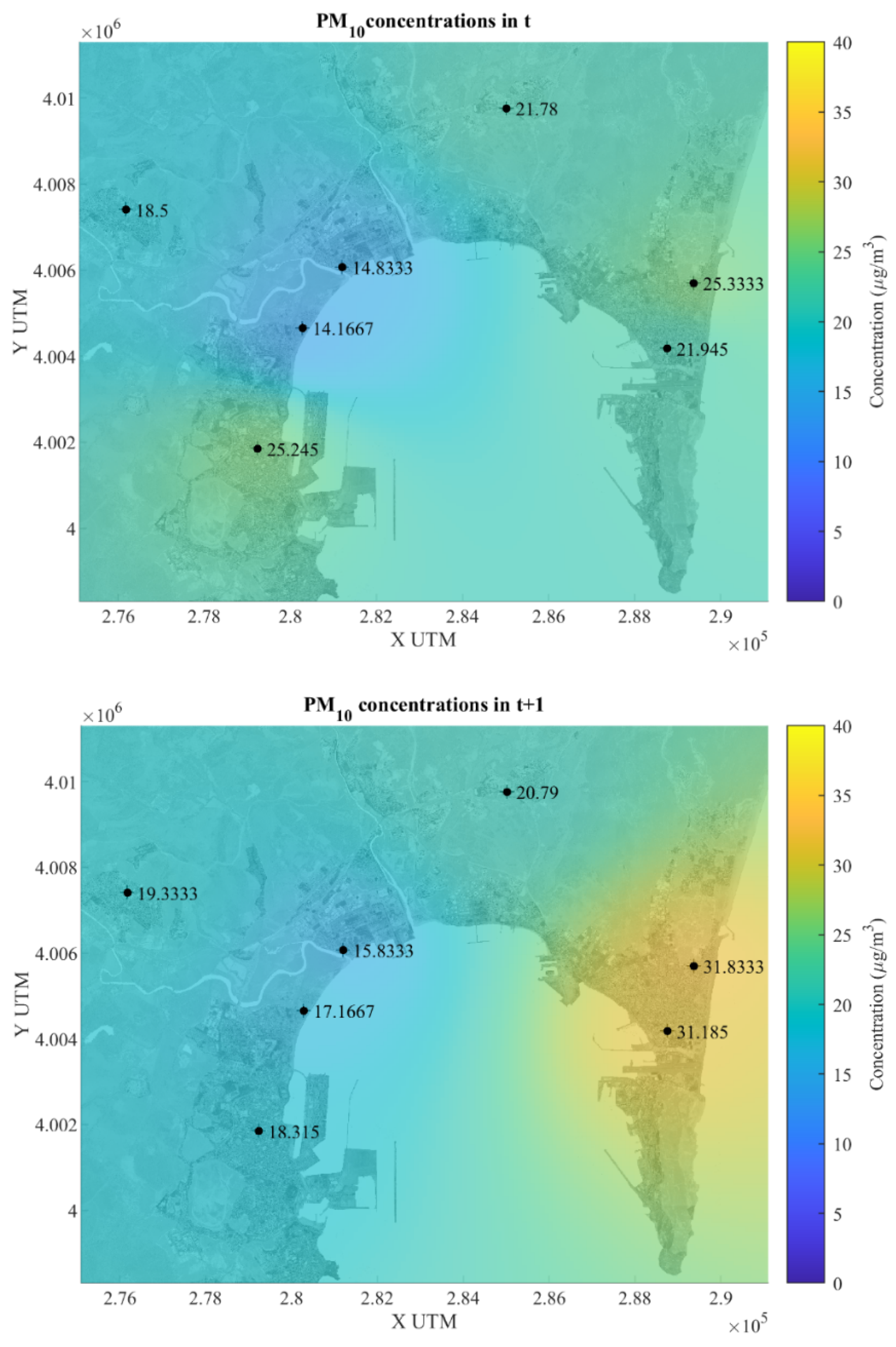
Figure 5 show an adequate performance to predict the behavior of PM
10 concentrations. If we examine
Figure 5 (real PM
10 concentration values in timestamps
and
, and also the prediction map for the timestamp
), a discernible ascending pattern is evident in the actual PM
10 concentration values (µg/m
3) at time
and one hour later (
). The highest increase happens in La Línea (station 13), going from 21.94 µg/m
3 to 31.18 µg/m
3 and a prediction of 42.54 µg/m
3. In the time series concentration maps, there is also an increase from 25.33 to 31.83 in El Zabal, station 10, and 14.16 to 17.16 in El Rinconcillo, station 7. Conversely, some stations exhibit a contrary downward trend, such as the shift from 25.24 to 18.31 in Algeciras, station 1, and 21.78 to 20.79 in Colegio Carteya, station 6. Regarding the one-hour forecast, the model yields relatively elevated values in certain stations, such as Algeciras, where the predicted value rises from the actual 18.31 in
time series to 30.51, and La Línea, escalating from the real value of 31.18 to the predicted 42.54. However, in nearly all other stations, the predictions demonstrate a decrease. This rise in pollution in the main cities of the Bay could be taken as a protection against decision making by both the population and the authorities.
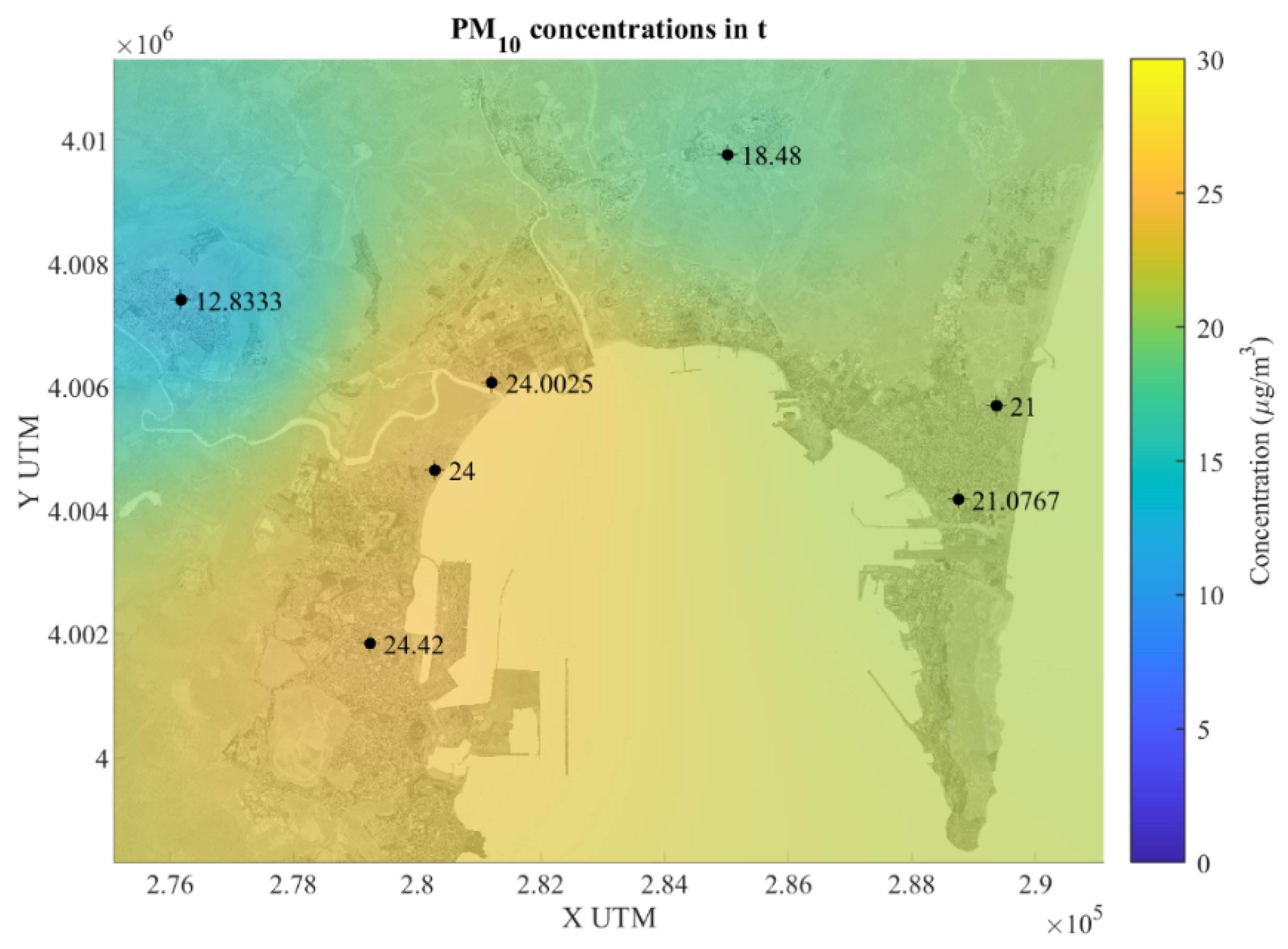
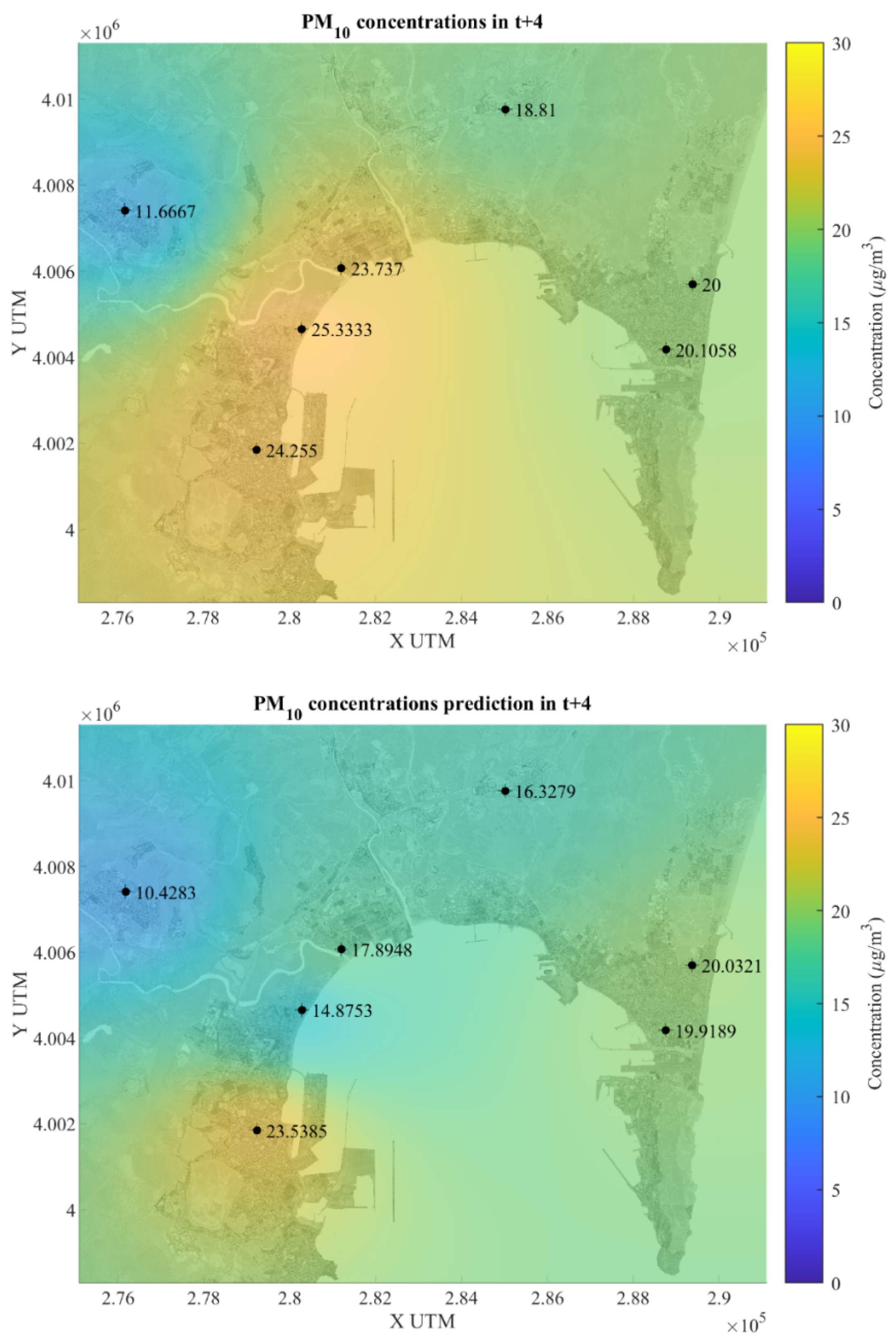
Observing
Figure 6, we appreciate that, in general, from the time series PM
10 concentration values at time
and four hours later,
, there is a decreasing trend in PM
10 pollution concentration values (µg/m
3) in almost all stations, except in El Zabal where there is a slight increase (from 20 to 20.03). In Algeciras, the values are almost imperceptible from 24.42 in
, 24.25 in
and a slight decrease in the prediction at
of 23.54.
It is predicted with quite good results 4 h ahead, and practically all stations show a similar trend in the predicted concentrations, which is promising and validates the goodness of the forecasting model.
The methodology used has been adequate to achieve the objectives of this work. The selection of the best model at each monitoring station statistically and comparatively has produced results above 0.85 in almost all cases. In addition, and above all, the use of jumps in the autoregressive scheme to predict at
produces very satisfactory results. The predictions at the locations of the monitoring stations have been combined with the IDW method to generate concentrations at each location
) of the region and the results show that the maps give us an interesting visualisation of the whole area and can be used for decision making by citizens or administrations. The predictions at each station vary because the historical time series of the pollutant differs across locations. This leads to slight differences in the optimal model for each station. For example, 1 station may require 5 neurons, while another may need 10, or it may require more or less historical data. This study is supported by similar research on the short-term prediction of PM
10 pollutants using non-linear variables. For instance, a study by [
38] demonstrated the effectiveness of ANN models in predicting daily PM
10 exposure, achieving an
R value of 0.81 for Vienna and 0.71 for Dublin. Notably, the results presented in this paper surpass these findings, achieving an
R value exceeding 0.85 even when incorporating historical data and considering prediction horizons of 1 and 4 h. Furthermore, our results show significant improvement over other similar studies, such as [
39], where an
R value of 0.78 was reported.
The results and methodology could be applied to any other area of study. We could even think of new techniques such as transfer learning [
40] to adapt the training to other scenarios, such as other locations or other prediction horizons.
5. Conclusions
The overall prediction results are quite good, with correlation coefficients reaching up to 0.845 across all stations and for both prediction horizons (1 h ahead and 4 h ahead) analysed. This indicates that the models predict with a high degree of accuracy.
The scheme presented in this paper is an effective procedure for the generation of air pollutant maps in a certain area, using, firstly, local prediction models at points in the area where historical time series data of pollutants are available, and, secondly, using a geostatistical interpolation method to estimate concentrations at other points where no data are available. Furthermore, it can be extended to other study areas.
The accessibility of these maps not only serves the scientific community and decision-makers but also enhances public awareness regarding pollution concerns and their possible consequences. By offering a lucid and user-friendly visualisation of intricate data, these dynamic maps function as a compelling educational resource, encouraging active engagement in the safeguarding and preservation of the natural environment.
This holistic approach showcases the capability of science and technology to tackle current environmental issues, fostering proactive measures for the well-being of human health and the entire ecosystem. This research aims to make these models comparable, thoroughly documented, and meticulously validated, to achieve reliable results.


 ,
, 


