Oil Spill Classification Using an Autoencoder and Hyperspectral Technology

Abstract

Hyperspectral technology has been playing a leading role in monitoring oil spills in marine environments, which is an issue of international concern. In the case of monitoring oil spills in local areas, hyperspectral technology of small dimensions is the ideal solution. This research explores the use of encoded hyperspectral signatures to develop automated classifiers capable of discriminating between polluted and clean water and distinguishing between various types of oil. The overall objective is to leverage these classifiers to be able to improve the performance of conventional systems that rely solely on hyperspectral imagery. The acquisition of the hyperspectral signatures of water and hydrocarbons was carried out with a spectroradiometer. The range of the spectroradiometer used in this study covers the ranges between [350–1000] (visible near-infrared) and [1000–2500] (short-wavelength infrared). This gives detailed information regarding the targets of interest. Different neural autoencoders (AEs) have been developed to reduce inputs into different dimensions, from 1 to 15. Each of these encoded sets was used to train decision tree (DT) classifiers. The results are very promising, as they show that the AE models encoded data with correlation coefficients above 0.95. The classifiers trained with the different sets provide accuracies close to 1.

1. Introduction

Hyperspectral technology has emerged as a leader in the field of monitoring, covering a broad spectrum of uses thanks to the remarkable advances and increasing availability that have been experienced in recent years [1]. This progress has consolidated the position of hyperspectral technology as a fundamental tool in various sectors. In particular, its relevance in oil spill monitoring stands out, where its ability to analyse and detect subtleties in spectral characteristics allows for more accurate and efficient monitoring [2].

Interest in oil spill monitoring dates back to 1954, when the first International Convention for the Prevention of Marine Pollution by Oil Spills (OILPOL) was enacted. This event marked the beginning of global efforts to address the negative impacts of oil spills on marine ecosystems. As the first marine pollutants to receive significant attention, oil spills led to the implementation of specific measures for their monitoring and reduction. This pioneering approach laid the foundation for future international conventions and protocols, such as The International Convention for the Prevention of Pollution from Ships (MARPOL), underlining the importance of global collaboration in safeguarding and conserving the oceans from oil pollution.

Nowadays, oil spill monitoring is even more important since the 2030 Agenda, resulting from the COP27, establishes Goal 14 “life underwater”, as a specific target for protecting 30% of the seas and oceans by 2030 [3]. Their significant consequences and far-reaching impacts [4], both in the marine domain and human activities [5,6], as well as the oceanic economy [7], place oil spills in the spotlight as one of the 32 main issues to be tackled by science before 2030 [8].

All the efforts made over the years have succeeded in reducing large (>700 t) and medium spills (700–7 t) to marginal amounts in European waters. However, small oil spills still represent significant volumes.

Visual identification of oil spills is often made difficult by their intrinsic characteristics, such as their wide dispersion and sometimes low density, the variability in lighting conditions, or the influence of environmental factors such as waves and wind. Some studies, such as Li’s [9,10], develop wind prediction models to determine the dispersion conditions of oil spills. However, the development of advanced monitoring systems to achieve accurate and real-time detection is required, thus ensuring an effective and prompt response to oil pollution incidents in marine environments to minimise the adverse effects associated with oil spills. This is even more important when it comes to controlling oil spills in local areas with a high risk of incidents, such as waters in port areas and/or bunkering and refineries.

Hyperspectral technology of small dimensions has emerged as an innovative solution to overcome these challenges due to the combination of the spectral resolution of the hyperspectral technology with its high spatial resolution and flexibility for true continuous surveillance of local areas, as it can be installed on unmanned aerial vehicles (UAVs). The distinctive optical characteristics of materials, coupled with advancements in technology and the accessibility of sensors [1], place hyperspectral imaging of small dimensions as a solution for the monitoring of water pollution in local areas.

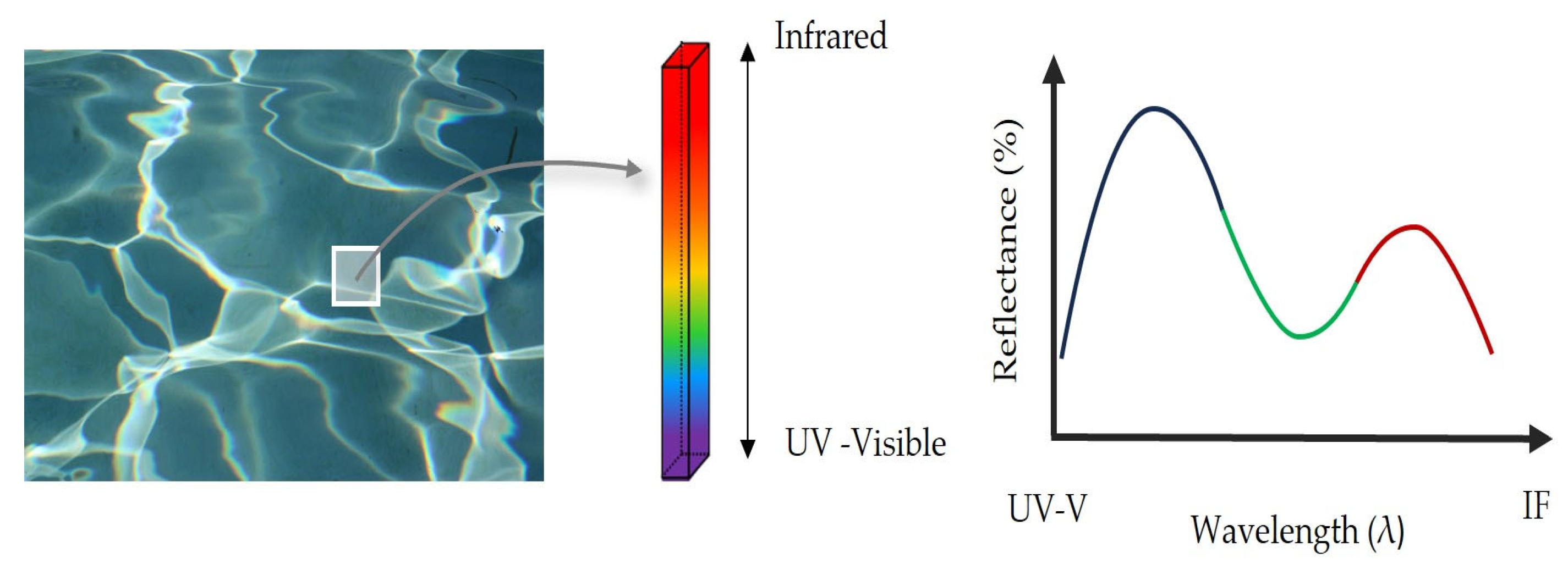
Hundreds of narrow and contiguous wavelength bands within the visible and infrared wavelength bands provide detailed spectral data. This rich and complete optical information defines quasi-continuous spectral signatures (Figure 1) that allow for identifying subtle differences between two similar targets at first sight. This capacity proves invaluable for the prediction of the thickness of oil film [11,12] as well as differentiating amongst seawater and oil films [13,14], among various other applications.

The development of a model based on hyperspectral signatures to control oil spills in local areas could help to improve the performance rates of a conventional system based solely on hyperspectral images. There is a wide range of techniques that can be used to classify targets according to the information embedded within the hyperspectral signatures [15,16,17]. Machine learning techniques can be applied to problems involving hyperspectral signatures since they represent one-point information without any other extra information. DTs are well-known classifiers, which have been extensively utilised in diverse fields [18], as well as in remote sensing [19,20].

A prior analysis of the relevance of hyperspectral signatures is convenient. This study provides information about the importance or contribution of each spectral band in the ability to distinguish or characterise different elements or phenomena in hyperspectral data. Hyperspectral data are characterised by the large volume of associated information, leading to high dimensionality. An analysis of the relevance of signatures allows for dimensionality reduction while retaining crucial information, thus simplifying the analysis. Furthermore, identifying the most relevant bands enhances the accuracy in classifying objects or materials, and by working only with the most relevant bands, the computational load can be reduced, thus improving analysis efficiency [21].

There are several research studies in which Principal Component Analysis (PCA) has been used successfully as a feature selection method for spectral responses [22,23]. However, the non-linear nature of spectral data [24] renders AE, also known as nonlinear-PCA, a much more convenient feature selection method in the remote sensing field [24,25]. AE has also been demonstrated to be a powerful tool for interpreting better and handling different types of data. Rodríguez-García et al. [26] apply AE for the further forecasting of SO₂, PM10, and NO₂ concentration. In the same way, Loy_Benitez et al. [27] use a variant of AE to develop a soft sensor validation technique. AE has also been employed in the field of chemistry, to create molecular representations [28], as well as in general industries, such as in intelligent fault diagnosis [29].

This research aims to stack a shallow AE and a DT classifier to create a model for the discrimination of hyperspectral signatures and to determine the dimensional reduction that provides the most optimal classification. Different shallow AEs will be tested to train different classifiers with each new projected dataset. A rigorous and comparative evaluation of the developed models will be conducted to determine their effectiveness in automatic classification. Multiple comparison techniques, such as the Bonferroni method and the Friedman test, will be used for the identification of differences in these methods. They will also be used to determine which were statistically superior. In Section 2, the preparation of samples is discussed. This section also discusses the method used for data collection and the shallow AE as well as DT classifier techniques and the multiple comparison methods including the Friedman test and the Bonferroni method. Section 3 shows the main results of this research. A discussion of the key findings of this work is provided in Section 4. A summary of the main ideas of this work is presented in the Conclusions Section.

2. Materials and Methods

The specific materials, tools, and equipment used for this research will be outlined here. Furthermore, the step-by-step procedures followed during the experiments will be explained, as well as the methodology.

2.1. Sample Preparation

This study was carried out under lab conditions in order to obtain an initial approach to the problem in a controlled environment.

Samples of both water only and hydrocarbon and water mixtures were included as part of the dataset samples.

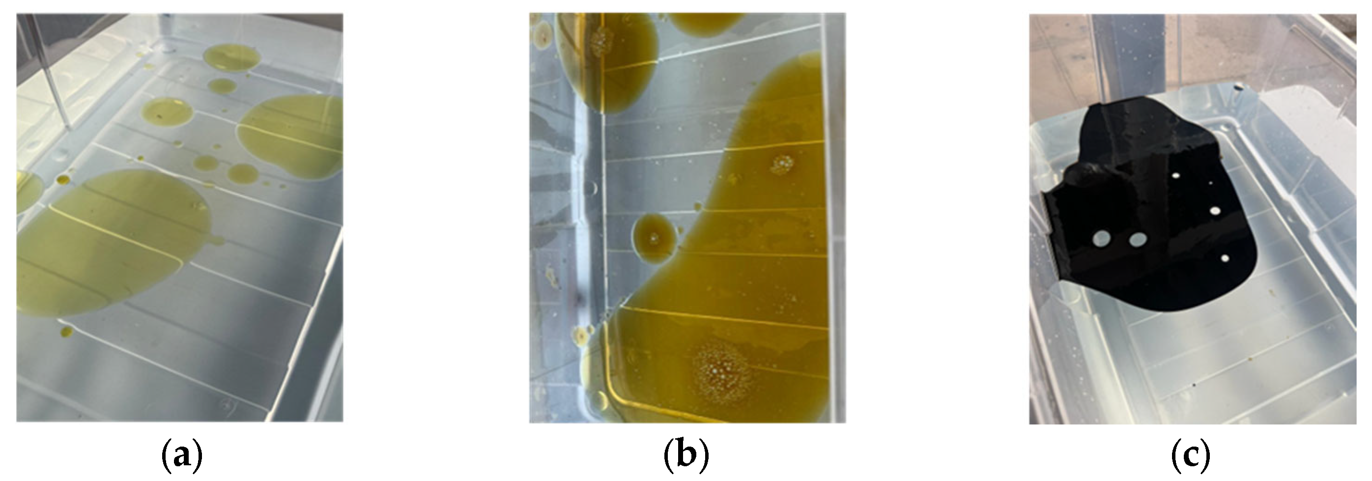
Real hydrocarbons that are susceptible to spills in marine areas were used to measure the performance level of the proposed method including the following: (a) diesel oil of vessels, (b) C10, and (c) high-sulphur fuel oil. Vessels and bunkering, among others, are possible sources of this type of oil entering the marine environment. These three hydrocarbons present different characteristics. Diesel oil is a hydrocarbon with a very low density and a yellowish colour when it is in high concentration. When it is spread over the entire surface, its appearance resembles that of water, forming rainbows. On the other hand, high-sulphur fuel oil is a very high-density hydrocarbon. Its colour is black and hardly spreads across the water’s surface. The oil C10 is an intermediate hydrocarbon, although is more like diesel oil than fuel oil. It is orange in colour when present in high concentrations but turns yellow as it spreads.

2.2. Dataset Acquisition

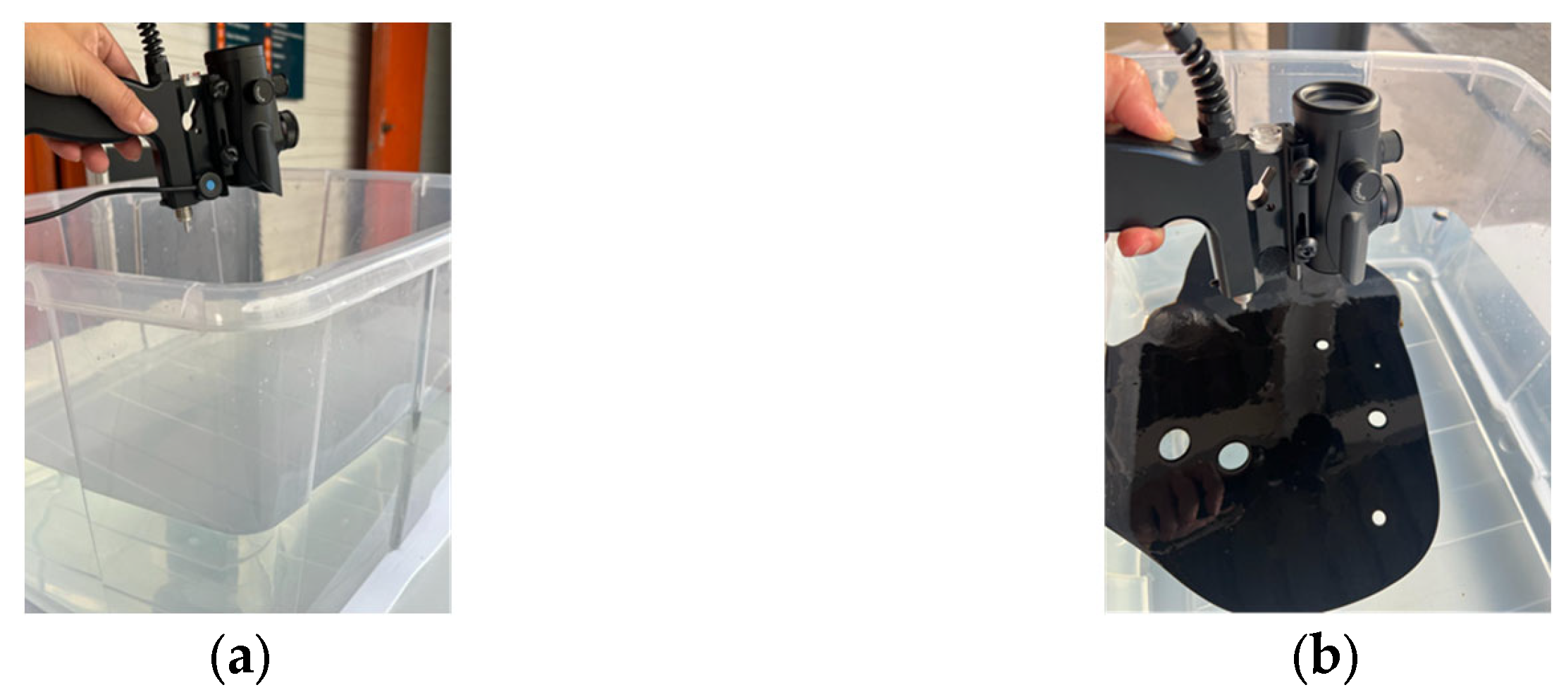
Hyperspectral signatures of water and the different oils and their boundaries were acquired with a spectroradiometer (Figure 2). This spectrometer was designed to enable the measurements of emitted, transmitted, absorbed, and reflected electromagnetic energy (EM) within the ranges of [350–1000 nm] (visible-near infrared) and [1000–2500 nm] (short-wavelength infrared). This instrument produces quasi-continuous signatures, as its bandwidth is less than 4 nm in some ranges. This electromagnetic information is collected by a set of optical fibres arranged in a gun-like handle. In this way, the hyperspectral signatures are point responses of the target to be measured.

Signature acquisitions were performed passively with the sun as the light source, ensuring that all spectral bands were available (Figure 3). The truthfulness of measurements was ensured by following the recommended techniques [30].

Reflectance was the optical property used to perform this research. To calculate the proportion of light that is reflected by the target, a previous measurement is required to determine the maximum quantity of light that is possible to reflect, i.e., 100% reflectance. For this purpose, a Lab spectralon board was used as a standard reference. This board acts as a white reference, providing a level of reflectance of almost 100% of the instrument’s range of work. Reference measurements were conducted at 5 min to ensure the precision of the signatures, including an initial measurement taken at the start of the experiment and the beginning of each hydrocarbon tested.

Two hundred and eighty sample spectrums were gathered. They included 40 water samples, 40 diesel oil samples of vessels, 40 samples of C-10, and 40 samples of fuel. A total of 40 samples of every boundary were also collected. All spectrums collected by the instrument correspond to the mean of 50 measurements.

2.3. Pre-Processing

The information provided by hyperspectral technology requires pre-processing before any subsequent analysis. In this initial stage, a specific part of the spectrum is selected to constrain the data. This reduction in the spectral range is necessary so that the results of the research can be applied as additional and complementary models to aid (such as a supplementary expert system) in the future when working with images acquired with a hyperspectral camera working in the VNIR range.

In addition, a normalisation process is carried out to counteract discrepancies in reflectance percentages, which can arise due to small variations in light intensity resulting from the position. This step is essential to ensure proper consistency and comparability in the data, establishing a solid basis for further analysis.

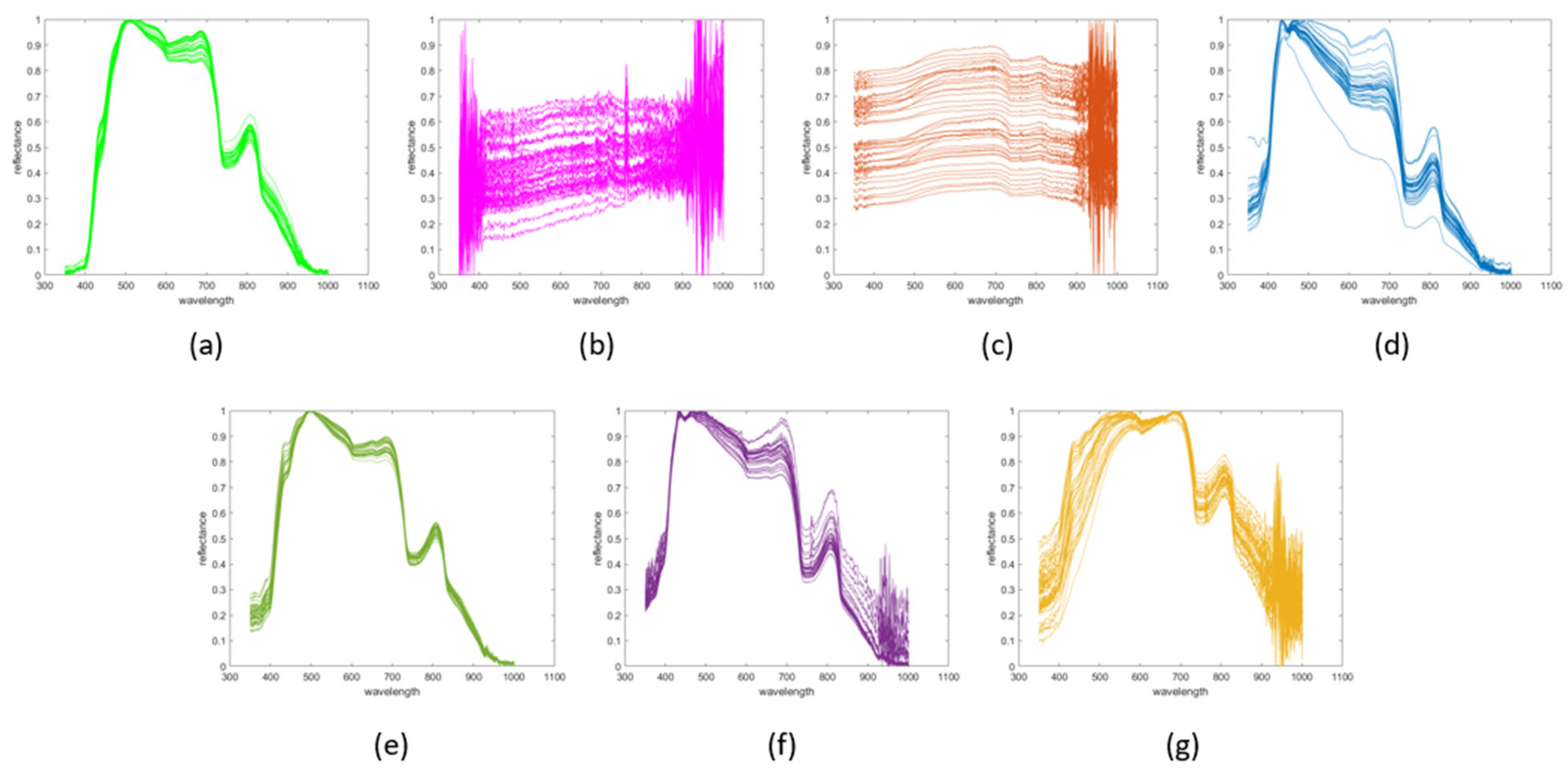
Figure 4 shows the final appearance of the hyperspectral trend signatures grouped by type of targets including the following: (a) diesel on water, (b) fuel oil on water, (c) C10 on water, (d) water, (e) diesel–water boundary, (f) fuel oil–water boundary, and (g) C10–water boundary, once the spectral range was reduced and the signatures were normalised. Each curve represents the spectral response of each measured point of the different targets.

2.4. Shallow Autoencoder

Once the pre-processing of the spectral signatures is completed, the first phase of the analysis begins, which consists of carrying out a relevance analysis using a shallow autoencoder. This step is crucial to identify and select the most informative features of the spectrum, allowing for a more efficient and compact representation of the data and effectively preparing it for more advanced analysis and subsequent modelling processes.

AE [31] is a well-suited technique for this task because, as a neural network model, it can learn complex patterns within the non-linear characteristics of spectral data [32]. AE is a particular case of pattern recognition where the outputs to be assigned are the inputs themselves. Both inputs and targets are identical data, and the outputs of the hidden layer serve as a non-linear encoded representation of the data. Consequently, the dimensions of the newly projected data are dictated by the number of hidden units used within the final hidden layer of the network model. In this work, compression was performed in one step so that the neural network consisted of a single hidden layer, as Figure 5 shows, as a shallow AE configuration.

The backpropagation neural network (BPNN) [33] stands out as the predominant neural model for pattern recognition. This is because it is trained based on the error that is propagated backwards to adjust the weight values of every neuron. Information is transmitted through a fully interconnected network starting at the input layer and moving towards the output one. The backpropagation method can be used to solve function approximation problems [34].

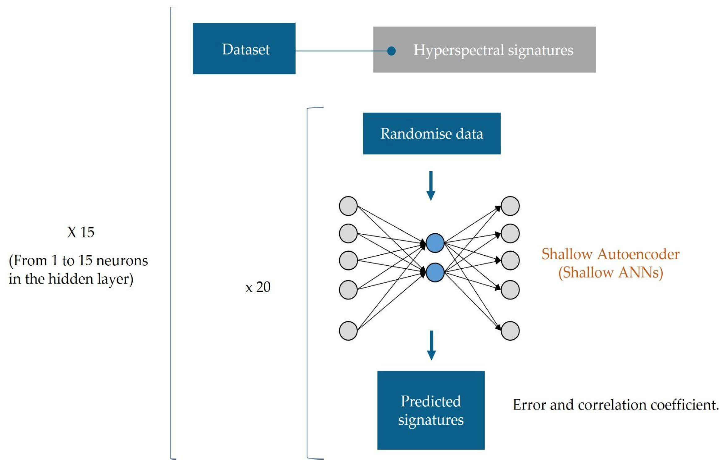
Different AE configurations were tested using different numbers of hidden units within the hidden layer. These ranged from a minimum of 1 to a maximum of 15 units to obtain new projected data in these dimensions. This approach allowed us to explore a diverse range of configurations, evaluating how the variation in the number of neurons affects the quality and efficiency of the compressed representations of the spectral data. Each configuration was trained 20 times, and the original database was randomly organised in each replicate. This process was intended to obtain the AE with the highest levels of generalisation capabilities and robustness. The number of hidden units was determined according to the desired dimension of the projected new database. The selection of the autoencoder for each dimension was based on the correlation coefficients obtained between the predicted and original signatures. Figure 6 shows the scheme used in the autoencoder calculation to obtain each of the new databases.

Following the assessment of the trained autoencoders, the original database was encoded in 15 different ways, resulting in new sets projected into spaces ranging from 1 dimension to 15 dimensions.

2.5. Decision Tree Classifier

DTs are supervised learning models that are inspired by a tree structure. Every internal node refers to a decision taken off a feature. Every branch represents a decision output. Finally, every leaf of the tree refers to a label value. In other words, a DT divides a dataset into smaller subsets based on the relevant features, intending to predict the target variable [35] accurately.

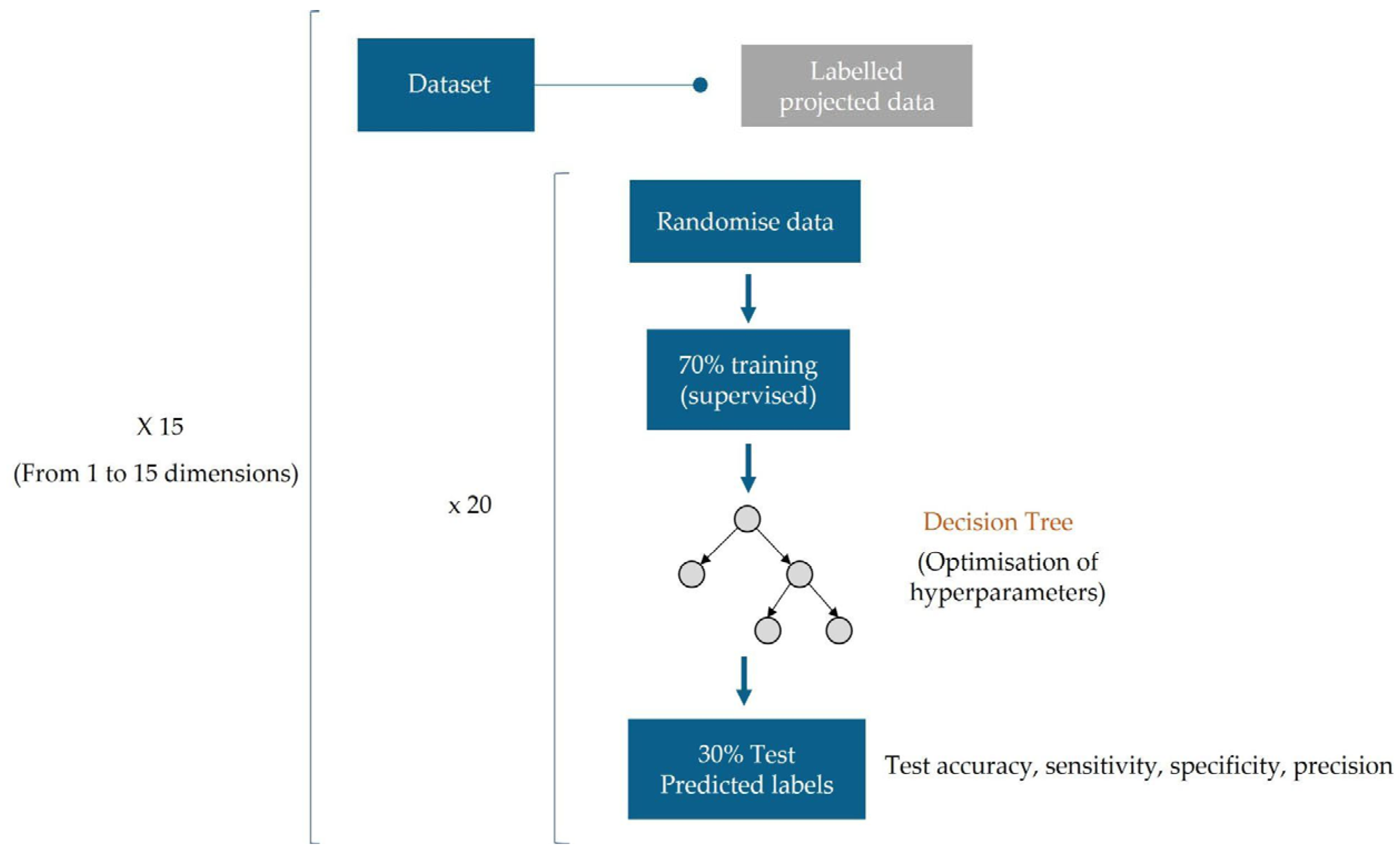
A total of 15 DT classifiers were developed, one for each new projected dataset (different units from within the hidden layer). Following the previous step, each classifier was trained 20 times, changing the inputs and hyperparameters each time to maximise the generalisation and robustness. First, input data were randomly organised to generate distinct training and test sets (70%–30%) for network training and testing purposes. The hyperparameters of the classifier were optimised at each attempt to achieve the best configuration for the DT classifier, minimising the cross-validation loss with which the training set was trained. The optimised hyperparameters were all eligible parameters, as listed below: (1) the maximum number of decision divisions (or branch nodes) that are integers; (2) the minimum number of leaf node observations, and (3) the split criterion. The classifier resulting from each iteration was evaluated using the test set, assessing metrics such as accuracy, sensitivity, specificity, and precision. The scheme followed in the calculation of the classifiers is presented in Figure 7.

2.6. Statistical Comparison

The developed models were rigorously evaluated and compared to determine their goodness of automatic classification and to assess which dimension of the projected data provides the best classifiers.

The Friedman [36] test was performed to statistically analyse the differences in the group means of accuracy, precision, sensitivity, and specificity obtained for the 20 replicates of the 15 classifiers. This test assesses whether there are significant differences between batches, i.e., whether the dimension on which to project the original dataset is significant.

Precision, sensitivity, and specificity parameters were evaluated for water classification, as this is the most relevant classification that the model must successfully achieve. The ultimate aim of the classified models is to be able to discriminate between polluted and clean water, representing a tool for environmental water monitoring.

The Bonferroni method [37] is a multiple comparison procedure used to identify differences in models and determine which are the best based on a statistical analysis. The accuracy levels obtained amongst the classifiers were evaluated.

3. Results

After performing the explained methodology, in which the pre-processed dataset of hyperspectral signatures of water, hydrocarbons on water, and their boundaries, was projected into new spaces of different dimensions, and their respective classifiers were trained, the main outcomes were summarised, highlighting the most significant results.

3.1. Feature Selection: Shallow Autoencoder

Table 1. Mean and standard deviation results using twenty replicates from the fifteen AEs.

Dimension of Projected Data	r (Mean)	Std Deviation
1	0.9087	7.54 × 10−7
2	0.9631	0.000471
3	0.9868	0.001809
4	0.9900	0.000368
5	0.9916	1.19 × 10−5
6	0.9927	0.000162
7	0.9935	0.000112
8	0.9938	0.000163
9	0.99424	0.000108
10	0.99450	0.000115
11	0.99472	9.65 × 10−5
12	0.99492	0.000130
13	0.99512	6.19 × 10−5
14	0.99530	0.000164
15	0.99539	0.000151

shows the results obtained after applying a shallow AE using a different number of hidden units to the pre-processed dataset of the hyperspectral signatures of water, oils on water, and their boundaries. This table represents the mean correlation coefficient of 20 attempts of each AE. Standard deviations of each correlation coefficient are also provided. This allows us to analyse the uniformity or disparity between the attempts of each AE.

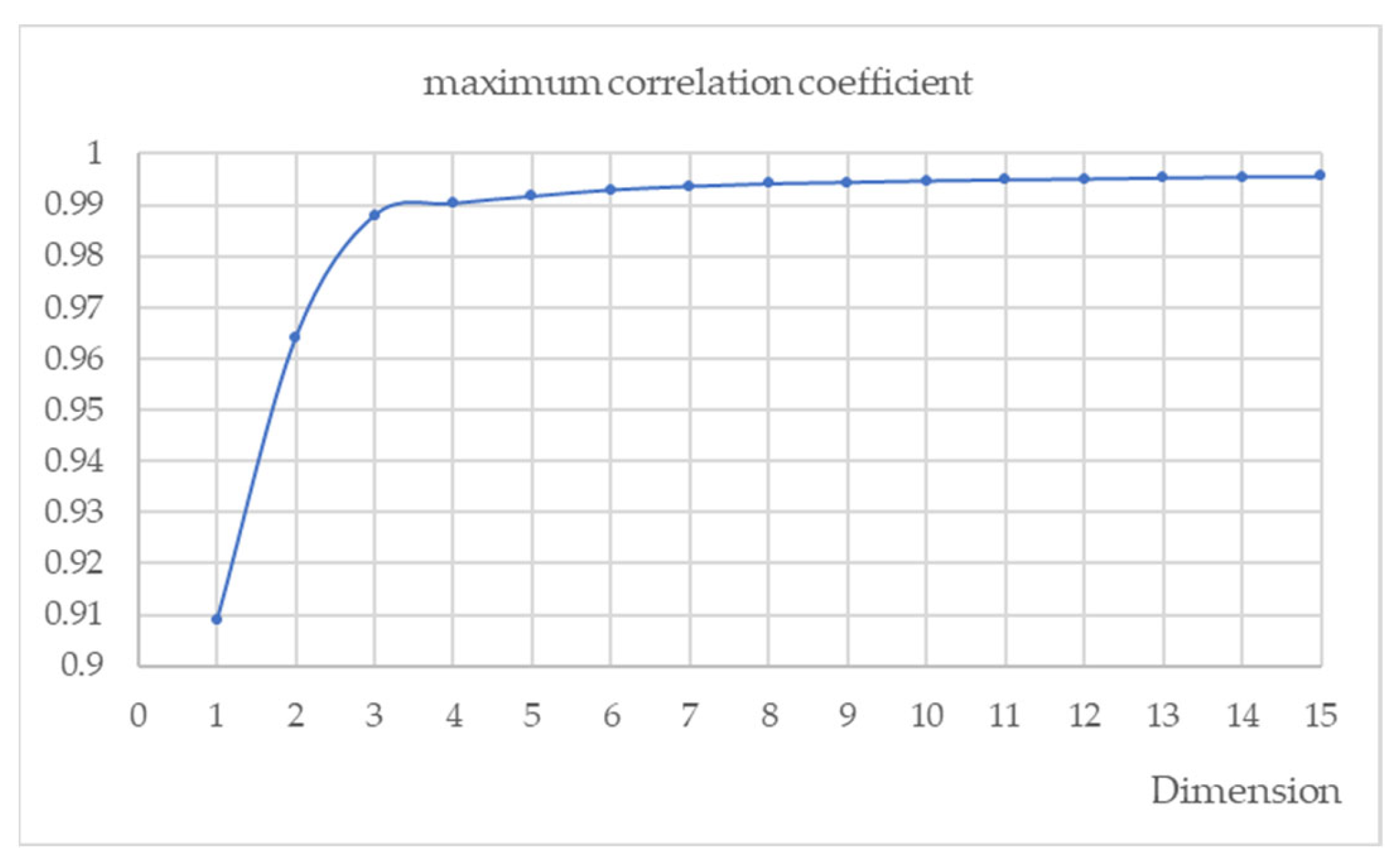
In addition to the mean values of the correlation coefficients, the maximum values obtained in each AE are also of interest. Figure 8 shows the values of the maximum correlation coefficients achieved in each AE. This representation provides a visual understanding of the evolution of the correlation coefficients regarding the number of hidden units used in the AE models.

3.2. Classification: Decision Trees

The mean results for accuracy, sensitivity, specificity, and precision of the 15 classifiers for the classification of water, the different oils on water, and their boundaries with the water are shown in

Table 2. Averages for accuracy, sensitivity, specificity, and precision of the 15 classifiers.

Dimension	Accuracy	Sensitivity	Specificity	Precision
1	0.8452	0.7050	0.9723	0.7842
2	0.7083	0.7750	0.9736	0.8078
3	0.9006	0.7700	0.9804	0.8599
4	0.8994	0.8100	0.9716	0.8121
5	0.9208	0.8200	0.9770	0.8381
6	0.9577	0.8250	0.9973	0.9771
7	0.9482	0.7850	0.9764	0.8393
8	0.9321	0.8150	0.9730	0.8139
9	0.9435	0.8550	0.9764	0.8496
10	0.9292	0.8500	0.9723	0.8138
11	0.9423	0.8100	0.9716	0.8208
12	0.9327	0.7950	0.9703	0.8089
13	0.9577	0.8900	0.9831	0.8893
14	0.9339	0.7950	0.9777	0.8508
15	0.9398	0.7800	0.9804	0.8578

. The best result is highlighted in bold.

Several statistical tests and methods were carried out in order to evaluate the different classifiers and to determine the best dimensional reduction to perform the model. This statistical analysis was carried out to evaluate the various classification parameters and to determine the presence of significant differences in these parameters as a function of the size of the inputs with which the classifier was trained.

Sensitivity, specificity, and accuracy parameters are related to the classification of water, which is the main target for identification by the models. This is essential for effective discrimination between contaminated and clean water.

Table 3. The Friedman test p-values, evaluating null hypothesis in the following three cases: (1) p-values obtained by applying the Friedman test to all the projected datasets (from dim. 1 to 15), (2) p-values obtained by applying the Friedman test to the projected dataset from dim. 2 to 15, and (3) p-values obtained by applying the Friedman test to the projected dataset from dim. 3 to 15.

Parameter	D1–D15 p-Value	D2–D15 p-Value	D3–D15 p-Value
Accuracy	4.86 × 10−26	1.95 × 10−20	9.42 × 10−13
Sensitivity	0.007091	0.089322	0.108005
Specificity	0.000132	0.000216	0.000274
Precision	3.74 × 10−5	0.000113	0.000231

presents the p-values produced after performing the Friedman test at the levels of sensitivity, generalisation, specificity, and precision of the 20 replicates of the 15 classifiers. Three different Friedman tests were carried out to enable the evaluation of the classification models without accounting for the impact of the encoded dataset that provided the worst coding. The first column shows the p-values resulting from the Friedman test and the classification parameter values of the 20 replicates of the 15 classifiers. The second column shows the p-values obtained after performing the Friedman test on the classifiers trained with the set of dimensions 2 to 15, leaving out the first dimension, which was the one that gave the worst correlation coefficient in the coding. The procedure was repeated to calculate the p-values of the third column, with the exclusion of the two first dimensions.

The accuracy levels after applying the Bonferroni method are presented in

Table 4. The Bonferroni method for accuracy. Evaluation of the significant differences among the different dimensional reductions regarding accuracy. C1: Dimension of the inputs. C2: Mean value of the evaluated parameter of the 20 repetitions of the classifier. Remaining columns: Classifiers for which there are no significant differences according to the Bonferroni method.

D	Mean	Non-Significant Differences
2	0.7083	2
1	0.8452		1
4	0.8994			4	3	5	10	8
3	0.9006			4	3	5	10	8	12
5	0.9208			4	3	5	10	8	12	14	15	11	9	7
10	0.9292			4	3	5	10	8	12	14	15	11	9	7	6	13
8	0.9321			4	3	5	10	8	12	14	15	11	9	7	6	13
12	0.9327				3	5	10	8	12	14	15	11	9	7	6	13
14	0.9339					5	10	8	12	14	15	11	9	7	6	13
15	0.9399					5	10	8	12	14	15	11	9	7	6	13
11	0.9423					5	10	8	12	14	15	11	9	7	6	13
9	0.9435					5	10	8	12	14	15	11	9	7	6	13
7	0.9482					5	10	8	12	14	15	11	9	7	6	13
6	0.9577						10	8	12	14	15	11	9	7	6	13
13	0.9577						10	8	12	14	15	11	9	7	6	13

. Column one specifies the dimension of the inputs, i.e., the dimension to which the original database was coded, with which the classifier was trained. The second column presents the mean value of the evaluated parameter of the 20 repetitions of the classifier. The remaining columns indicate the classifiers for which there are no significant differences according to the Bonferroni method.

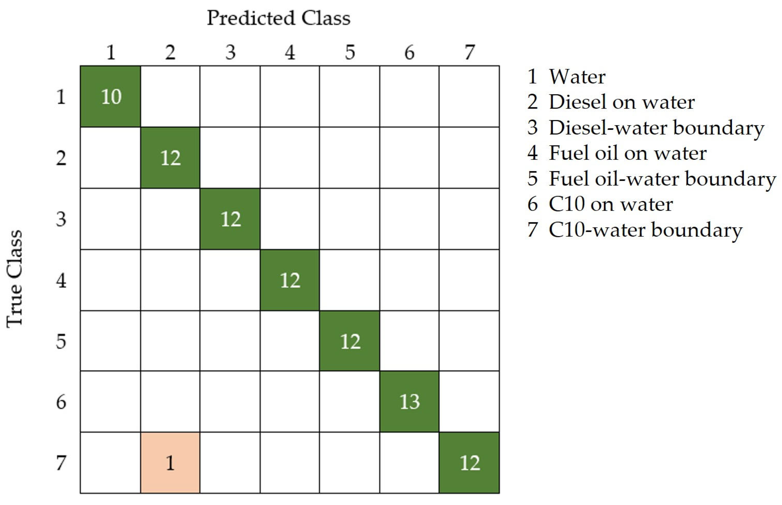
The statistical comparison indicates that the best classifier is the one using six-dimensional encoded data as input (highlighted in bold), with a mean accuracy of 0.9577 for the 20 replicates. The effectiveness of this classifier in the discrimination of the different targets, including water, diesel on water, C10 on water, fuel oil on water, and their boundaries, is presented with the confusion matrix of the test group (30% of the input) in Figure 9. The best replicate of the classifier trained with six variables as input, with an accuracy of 0.9881, only misclassifies one hyperspectral signature of the C10–water boundary, being identified as diesel on water, achieving a perfect detection of polluted water.

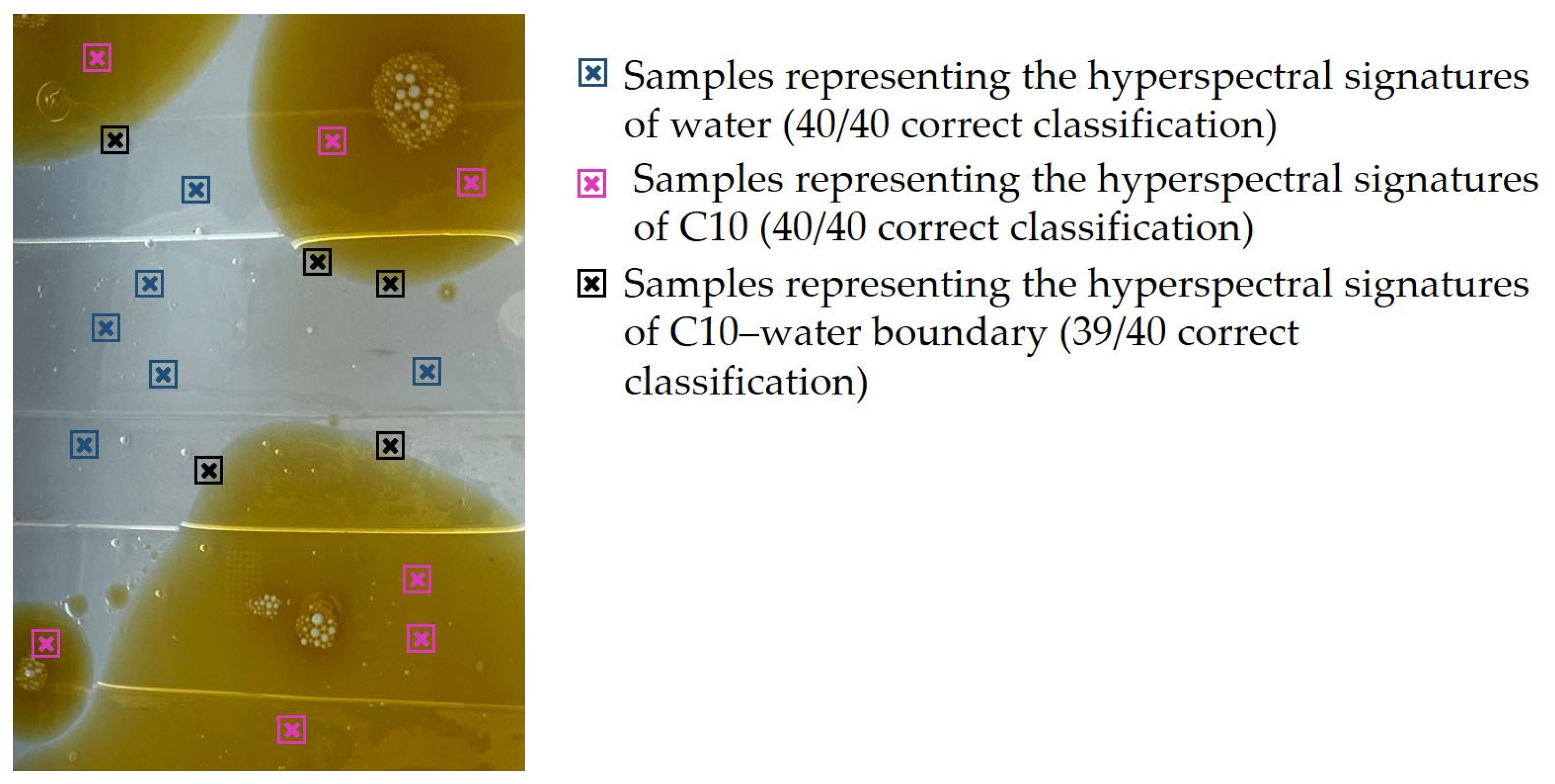
In addition to this, Figure 10 shows a visual representation of the C10 experiment in water. This figure displays a subset of the 120 samples belonging to hyperspectral signatures representing the following three classes: water (40 samples), C10 (40 samples), and the C10–water boundary (40 samples). All the polluted water samples were correctly classified, and only 1% of the water boundary samples were misclassified.

4. Discussion

The results presented in Table 1 about the different codifications of the original database offer two interpretations. On the one hand, regarding the means of the correlation coefficients, the larger the size of the projected space, the higher the correlation coefficient obtained. AE with more neurons keeps more original information. This finding is to be expected, and this is the reason for the subsequent analysis of the classifiers: to determine the optimal dimensionality reduction. On the other hand, regarding the standard deviations of these means, their low values show that there are no major differences in coding ability between the replicates of each classifier. Consequently, the replicate with the highest correlation coefficient of each classifier was selected to encode the original database, resulting in 15 encoded datasets.

There is one more interpretation that can be made of the feature selection task regarding the highest correlation coefficients for each classifier. The visual representation displayed in Figure 7 shows that dimensions larger than three do not provide a significant difference in the encoded process. However, the determination of the optimal dimension for the classification task with which to code the original database was performed through rigorous statistical analysis.

The results of the classifiers in Table 2 show that DT classifiers have a very good predictive capability. They reach values of accuracies close to 1, and they also present high levels of specificity and precision in the classification of water.

The Friedman test yields really interesting results (Table 3). There are significant differences among the classifiers when all 15 classifiers are tested, regardless of the classification parameter evaluated. This difference is most pronounced when it comes to accuracy. As the tests are reduced to the classifiers trained with the best-encoded inputs, the p-values increase. This increase in p-values in the second and third columns means that the classifiers trained with the 1-D and 2-D sets have associated poor performance. Nevertheless, p-values remain low in terms of accuracy.

This conclusion is clearly shown in the results of the Bonferroni method (Table 4). Inputs of 1-D and 2-D provide the classifiers with the worst accuracies and, moreover, no other is significantly similar to them. At the other extreme are the trained classifiers with encoded inputs to 6 and 13 variables. Both have the same mean accuracy, the highest of the 15 classifiers. Furthermore, the Bonferroni method explains that there are no inputs of dimension less than six that generate a classifier statistically similar to this one. Consequently, the optimal encoding corresponds to reducing the original database to six variables, i.e., an AE with six neurons in its hidden layer.

The best replicate of the trained classifier with six variables achieves an accuracy of 0.9881, misclassifying only one hyperspectral signature of the C10–water boundary as diesel out of the eighty-four hyperspectral signatures in the test dataset (Figure 9 and Figure 10). This means that a classifier with only six variables as input can perfectly classify 100% of polluted water.

5. Conclusions

In conclusion, the results of this research underline the effectiveness of AE in extracting key features from hyperspectral data and reducing their dimensionality. Remarkable correlation coefficients above 0.99 were achieved using AEs with only four neurons in their hidden layer.

Furthermore, it was proven that a basic classifier, such as DT, with a reduced dataset, can perform classifiers with accuracies very close to 1.

In addition to this, through the statistical analysis of the computed classifiers, it was demonstrated that more information is not associated with better classification results.

This knowledge could lay the foundation for future research in which the developed machine learning classifier based on hyperspectral signatures of water and hydrocarbons on water can be applied as a complementary and combined model for the real-time detection of oil in water in hyperspectral imagery of local areas.

The main disadvantage of using a spectroradiometer as prior knowledge of the different targets, such as water and hydrocarbons, lies in the fact that this instrument cannot be used for continuous monitoring of water because of its dimensions. However, the information derived from hyperspectral signatures can enhance the performance of a traditional system that relies exclusively on an imaging system with a hyperspectral camera on board a UAV, and it could also make computational improvements.