Article

Application of Modified BP Neural Network in Identification of Unmanned Surface Vehicle Dynamics

School of Information Engineering, Shanghai Maritime University, Shanghai 201308, China
*
Author to whom correspondence should be addressed.
J. Mar. Sci. Eng. 2024, 12(2), 297; https://doi.org/10.3390/jmse12020297
Submission received: 18 December 2023 / Revised: 3 February 2024 / Accepted: 4 February 2024 / Published: 7 February 2024

Abstract

:
Over the past few decades, unmanned surface vehicles (USV) have drawn a lot of attention. But because of the wind, waves, currents, and other sporadic disturbances, it is challenging to understand and collect correct data about USV dynamics. In this paper, the Modified backpropagation neural network (BPNN) is suggested to address this issue. The experiment was conducted in the Qinghuai River, and the receiver collected the data. The modified BPNN outperforms the conventional BPNN in terms of ship trajectory forecasting and the rate of convergence. The updated BPNN can accurately predict the rotational velocity during the propeller’s acceleration and stability stages at various rpms.

1. Introduction

Unmanned surface vehicles (USVs) have recently garnered significant interest from researchers and developers. Compared to traditional manned vehicles, the USV’s ability to operate in severely hazardous environments is one of its most remarkable advantages. USVs can perform tasks that conventional ships cannot achieve in terrible ocean environments and other situations. At the same time, these types of ships are of great importance for national defense security and environmental monitoring. However, controlling Unmanned surface vehicles is a notoriously challenging task that remains poorly understood due to various uncontrollable phenomena, including wind, wave, current, and other random disturbances. The unpredictability and dynamic nature of these external forces render the control of USVs particularly intricate. This is further compounded by the complex interactions between these disturbances and the vehicle’s dynamic characteristics. To compound the matter even further, USVs are often required to perform precise maneuvers in cluttered environments, which requires a high level of control authority and adaptability. To address these challenges, researchers have been exploring innovative control strategies that can enhance USV performance in hostile environments. These strategies often combine traditional control techniques with advanced algorithms and machine learning methods to develop more robust and adaptive control systems. Additionally, the use of simulation platforms has become an essential tool for testing and validating these control strategies before deploying them in real-world scenarios. In Antonelli’s research, it has been shown that using artificial intelligence algorithms for data processing has certain pattern recognition capabilities and can be analyzed without a physical model. However, this method currently lacks a comprehensive scientific explanation and cannot be falsified. However, he believes that data-driven artificial intelligence algorithms are still very worthwhile to study [1].
Numerous studies have been conducted to explore the control methods of Unmanned Surface Vehicles (USVs). The identification of the dynamic coefficient of the unmanned vessel plays a decisive role in the accurate motion control and automatic driving of the unmanned vessel, especially in the case of external interference. At present, no unmanned vessel can have accurate control ability in complex waters, which is also one of the problems of dynamic identification of hydrodynamic coefficients. The most common technique for handling an indescribable system from input–output data is system identification. In the process of system identification, Nagumo and Noda utilized continuous least squares estimation with error-correcting training [2]. Holzhuter employed recursive least square estimation to identify ship dynamics [3]. Kallstrom and Astrom demonstrated the use of recursive estimation of maximum likelihood in ship steering motion in 1981 [4], yielding well-predicted outcomes. To anticipate motion variables, hydrodynamic force, vehicle speed, and current direction, Yoon and Rhee suggested the extended Kalman filter approach and modified Bryson–Frazier smoother [5]. Shin et al. combined Particle Swarm Optimization (PSO) with an adaptive control technique to anticipate the trajectory of autonomous surface vehicles [6]. Additionally, Selvam described a frequency domain identification system for linear steering equations in ships’ maneuvering under calm seas [7].
Daniele’s research shows that it is very difficult to establish the dynamics model of both USV and ROV. The system delay problem of the dynamic system and the interference of the external environment lead to the failure of accurate control. Therefore, adaptive control algorithms, especially data-driven algorithms, are needed to solve these problems [8]. The dynamic model of ship dynamics poses a formidable nonlinear challenge due to the influence of wind, ocean currents, and various arbitrary disturbances. The nonlinear issue that emerged last year was successfully addressed through the application of Artificial Neural Networks (ANN). In order to tackle the system identification challenges posed by large oil tankers, Rajesh and Bhattacharyya proposed an artificial neural network approach [9]. The network was trained using the Levenberg–Marquardt algorithm, and multiple hidden neuron densities were evaluated to determine the optimal configuration. Oskin et al. introduced Recurrent Neural Networks (RNN) for identifying both linear and nonlinear behaviors in ship dynamics [10]. Additionally, Pan et al. employed an effective Neural Network (NN) method to track the movements of autonomous surface vehicles with unknown ship dynamics [11]. This series of studies provides crucial insights and innovative approaches for understanding and addressing the complexity of ship dynamics.
This study utilized a Back Propagation Neural Network (BPNN) to address the nonlinear dynamics problem of Autonomous Underwater Vehicles (AUVs). The benefit of the BPNN is that it has a robust non-linear mapping capability and a flexible network topology, making it ideally suited to the problem of vessel dynamic system identification. However, the traditional bp neural network has the ability of self-adaptation and self-learning and has strong nonlinear mapping ability, but it also has some defects such as slow convergence and easy fall into the local optimal solution. The additional inertia method and the adapted learning rate method are also chosen to improve the BPNN method in order to minimize these shortcomings. The training data comes from actual experiments that were conducted in the Qing-Huai river.
In order to study the motion control ability of the BPNN algorithm in USV, the algorithm is designed to take the speed of the left and right thrusters as input and output the surge velocity, swing velocity, rotation velocity, and trajectory through black box calculation, which can realize the motion control solution of USV. The above parameters are selected as input and output because these data can be obtained on the experimental model or can be calculated. This study includes two hidden layers. Through the expert experience method, the weight of the hidden layer is assigned, and the various parameters are correlated.

2. USV Dynamic System

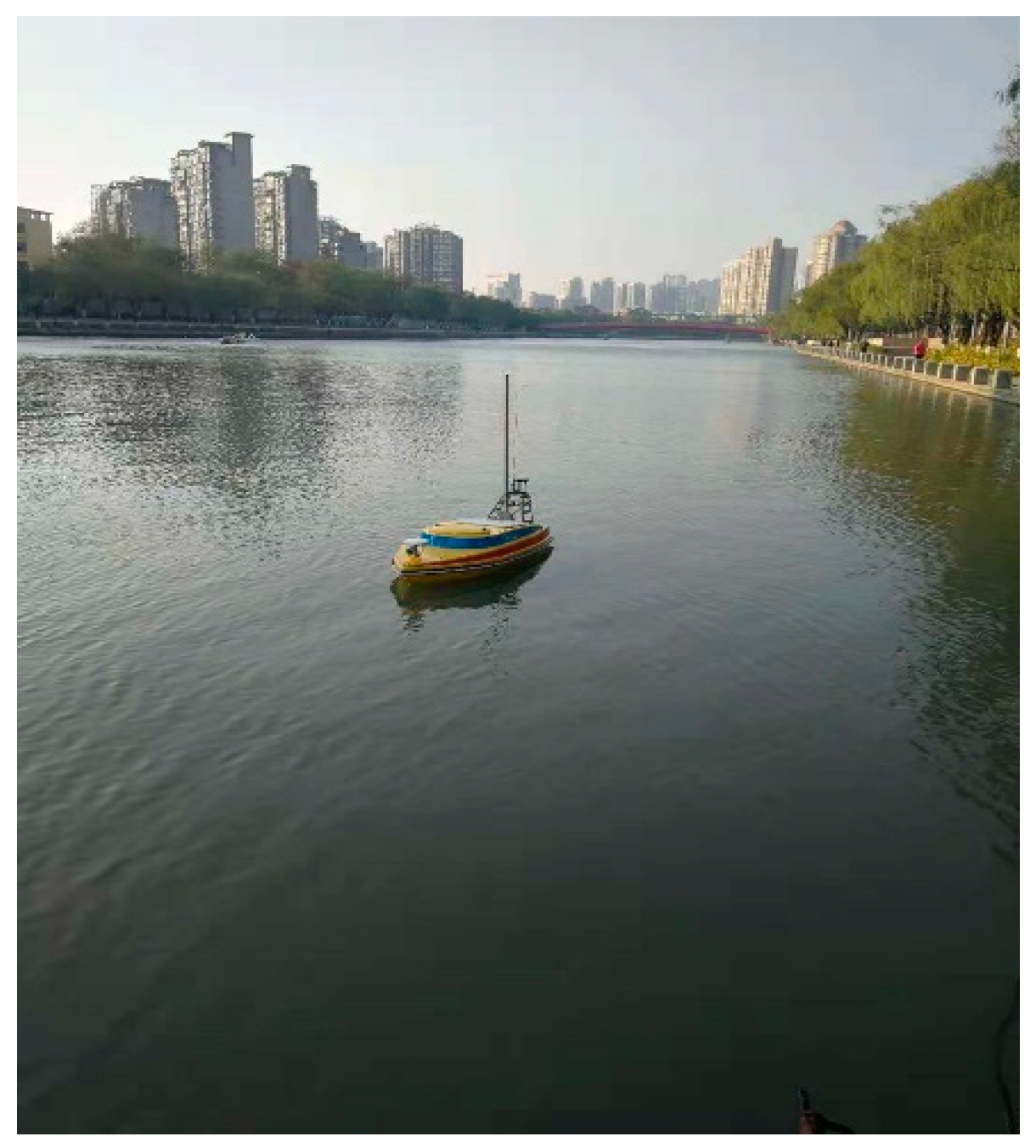
2.1. Deepsea Warriors uBoat (YL1300M)

We propose the following development requirements for the USV to be able to perform algorithm verification in a real environment. The real ship is shown in Figure 1.
a.
The body of the YL1300M is shaped to be more streamlined in order to reduce resistance.
b.
The YL1300M must have good stability in order for the USV to function in a freshwater and inshore environment.
c.
The vessel features a sizable storage area for carrying a variety of tools and supplies.
d.
The boat’s upper deck features a sizable cover that can be used to disassemble and repair equipment.
e.
There are two electric propulsion modules in the car. Due to the lack of a rudder and gimbaled thruster on the YL1300M, the steering motion can be produced by altering the RPM (revolutions per minute) of the two primary thrusters.
The YuanLi-1300M measures 1.3 m in length, 0.64 m in width, and 0.55 m in height. The vehicle is equipped with various sensors, including two differential GPS units located at the bow and stern, respectively, as well as an electronic compass capable of measuring position, speed, and heading angle.

2.2. USV Dynamic Model

In Marco’s paper, the rigid-body dynamics equations for the UUV are described. He described the motion of the vehicle as an equation of six degrees of freedom. When considering the influence of the external environment, the coupling relationship is ignored and only the simplified uncoupling model is considered [12]. In order to characterize the motion of the USV in a simple manner, the three degrees of freedom (surge, sway, and yaw) in horizontal planar motion are taken into account in this work. The USV and its coordinate frame are described in Figure 2 using the nomenclature proposed by Fossen [13].
The u ,   v , and V indicate the upsurge, swing, and overall speed of the USV in a body-fixed frame, respectively while the x i ,   y i denote the north and east direction of the USV in the inertial frame, respectively. In addition, ψ and β denote the heading angle and course angle of the USV, respectively while X represents the side slip angle.
The kinematic model of the USV can be expressed as follows [14]:
η ˙ = R ( η ) v ,
v = ( u , v , r ) T ,
η = ( x i , y i , ψ ) ,
R ( η ) = cos ( ψ ) sin ( ψ ) 0 sin ( ψ ) cos ( ψ ) 0 0 0 1 ,
where indicates the velocity vector v, the position vector η, and the rotation matrix R(η) that maps the vector from the object’s fixed coordinate system to the inertial coordinate system.
The surface vehicle’s planar dynamic model can be explained as follows:
M v ˙ + C ( v ) v + D ( v ) v = f ,
where M indicates the mass matrix, which consists of the body’s mass and included mass, C(v) indicates the Coriolis and centripetal matrices, D(v) indicates the damping coefficient matrix and the present matrix Equation (6). Given that the YL1300M ‘s propulsion system is a differential thruster type, Sonnenburg et al. describe it as follows [15]:
f = τ X τ Y τ N = T p o r t + T s t b d 0 T p o r t T s t b d B / 2 ,
where T p o r t and T s t b d denote the port side thruster’s thrust force and the starboard side thruster, respectively. B the beam of the YL1300M.
Consequently, the following is an illustration of the three degrees of freedom nonlinear dynamic motion equations:
m X u ˙ u ˙ m ( x G r 2 + v r ) + Y v ˙ v r + Y r ˙ + N r ˙ 2 r 2 + X u u + X u u u u = τ X ,
( m Y v ˙ ) v ˙ + ( m x G Y r ˙ ) r ˙ + ( m X u ˙ ) u r + Y v v + Y r r + Y v v v v + Y r r r r = τ Y ,
m x G N v ˙ v ˙ ( I z z N r ˙ ) r ˙ + m x G u r Y v ˙ u v Y r ˙ + N r ˙ 2 u r + X u ˙ u v + N v v + N r r + N v v v v + N r r r r = τ N ,
where X · , Y · , and N · in Equations (7)–(9) represent constant hydrodynamic coefficients, which are partial derivatives of surge, sway force, and yaw moment, respectively.

3. Neural Network

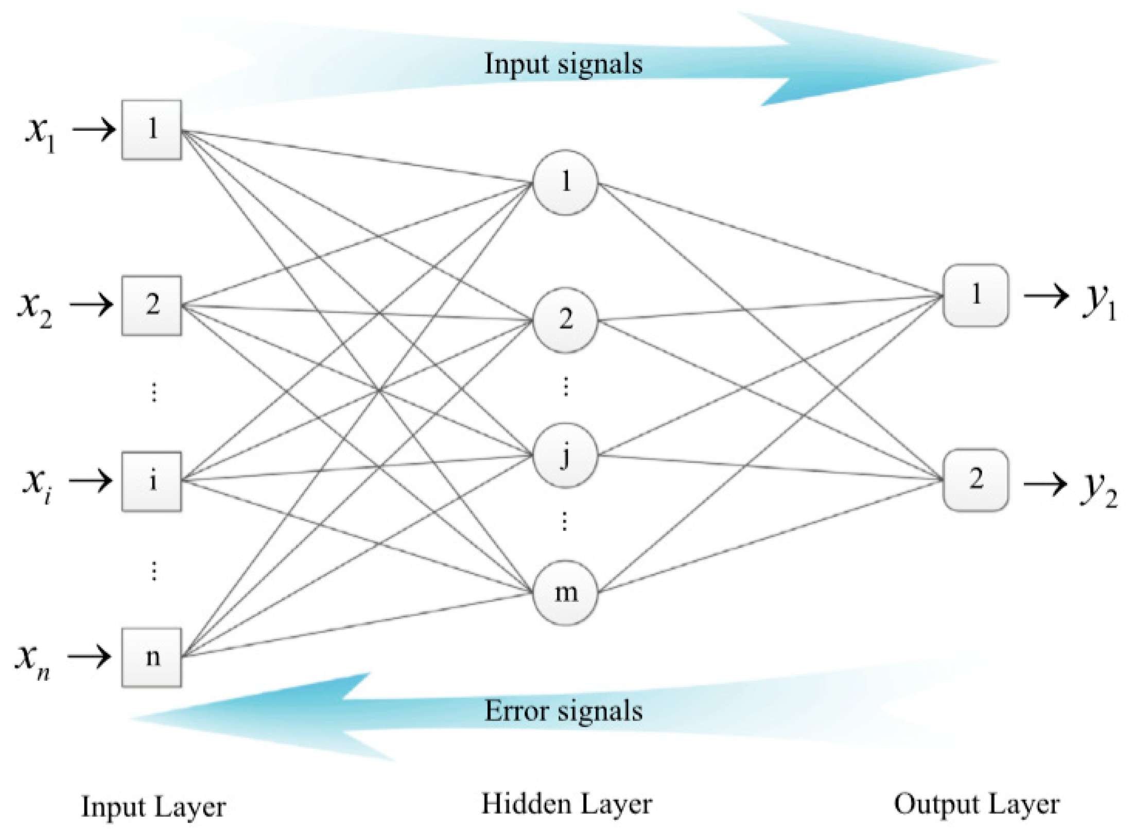
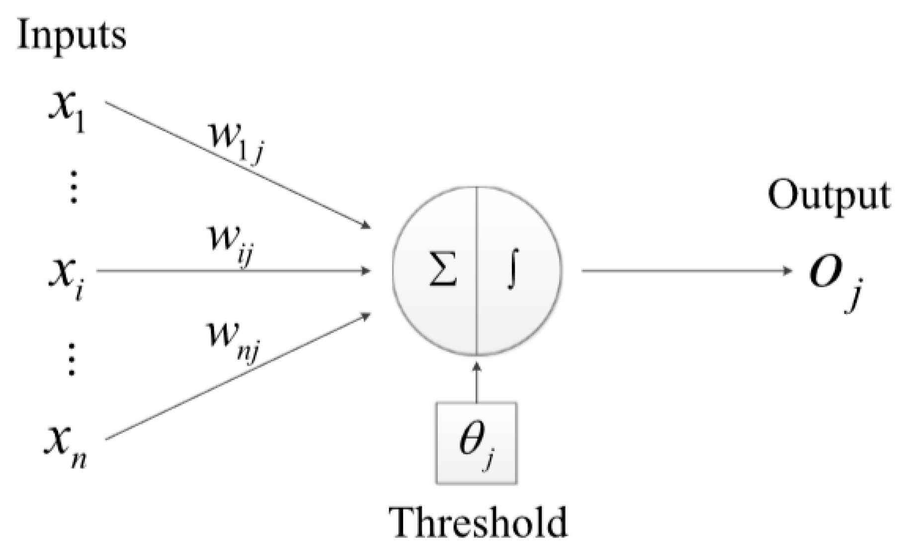
3.1. The Back Propagation Neural Network Principle

In 1986, the back propagation neural network (BPNN) was proposed by Rumelhart and colleagues and McClelland. The input layer, hidden layer, and output layer of the BPNN are depicted in Figure 3. The relationship between the number of the input layer, hidden layer, and output layer may be understood using the empirical formula given by Li et al. [16]:
M = N + K + φ ,
where indicates the hidden layer’s unit number, N the input layer’s unit number, K the output layer unit number, and φ a constant number that falls within the (1, 10). φ is set to 5.
Back propagation and forward propagation are two of the methods used in BPNN. The outcome of the neural network can be obtained during this process to be contrasted with the intended data; this discrepancy is regarded as an error and is employed in the backward propagation process to generate the loss function valve. The input data is propagated from the input layer to the output layer. Using optimization techniques, the link weights and threshold can be changed to reduce the loss function.
As can be demonstrated in Figure 4, Assume n input signals are propagated in a neural unit j, and the following is the way the result can be determined:
O j = f i = 1 n x i w i j θ j ,
where w i j represents the value of the weight coefficient of friction, θ j the neural unit’s threshold, f · an activation function, and the Sigmoid function are used, as shown below:
f ( X ) = 1 1 + exp ( X ) ,
Substituting Equation (12) into Equation (11) and the output O j can be expressed as:
O j = 1 1 + exp i = 1 n x i w i j θ j .
The neural network’s i - th output value is compared to the real value, and the difference is known as the unit error of the output layer. Its error function is depicted below:
E i = 1 2 k = 1 k y d , k y k 2 ,
where y d , k and y k denote expected value and real value of neural unit k, respectively, within the output layer. The entire mistake E for m samples of training is expressed as follows:
E = 1 m i = 1 i E i .
The malfunction indicator is obtained layer-by-layer via recursive propagation and the weights will be adjusted to reduce the error. The next will show that how to adjust weights to decrease the error. In the p-th iteration, the mistaken indioncate of the output layer of neuronal cells unit k is as follows:
e k p = y d , k p y k p .
Then the error will be utilized to modulate the weight in the next iteration and can be shown as:
w j k p + 1 = w j k p + Δ w j k p .
However, Equation (17) is not able to maintain the accumulation of the learning experience which means the velocity of the convergence is slow. This paper adopts the additional momentum method, which is as follows:
w j k p + 1 = w j k p + Δ w j k ( p ) + α w j k ( p ) w j k ( p 1 ) ,
where α denotes the rate of the momentum learning.
The adjusting part of the weight Δ w j k ( p ) can be calculated as:
Δ w j k p = η × y i p × λ k p ,
where η denotes the learning rate, y i ( p ) the output signal of neuron unit j, and λ k ( p ) the error gradient of neuron unit k.
The standard η is belonging to (0, 1), but the η is difficult to determine, if the η is too large which result in generating the oscillation in the learning process while the η is too small which cause the velocity of convergence become slowly. The adaptive learning rate method is adopted which can be shown as follow:
η ( t ) = η max ( η max η min ) × t t max ,
where η max indicates the highest rate of learning, η min the lowest possible rate of learning, t max the greatest quantity of iteration, and t the current number of iteration.
The error gradient can be calculated as:
λ k ( p ) = y k ( p ) X k ( p ) × δ k ( p ) ,
where X k ( p ) denotes the neural unit’s weighted input k, δ k ( p ) the error of the neural unit k. If neural unit k is in the output layer,
δ k ( p ) = e k ( p ) .
Figure 5 demonstrates the error gradient’s back-propagation process for a unit and the error of the neuron can be written as:
δ K ( P ) = i = 1 l δ i ( p ) × w k i ( p ) ,
where l denotes the result of the layer’s neural unit count.
In Equation (21):
y k ( p ) X k ( p ) = 1 1 + exp X k ( p ) X k ( p ) = exp X k ( p ) 1 + exp X k ( p ) 2 = y k ( p ) × 1 y k ( p ) .
Substitute Equations (21)–(23) into Equation (24):
When the output layer’s neural unit k:
λ k ( p ) = y k ( p ) × 1 y k ( p ) × e k ( p ) .
When the hidden layer’s neural unit k:
λ k ( p ) = y k ( p ) × 1 y k ( p ) × i = 1 l δ i ( p ) w k i ( p ) .

3.2. BPNN for Dynamic Model Identification

According to Equations (7)–(9), The thruster force determines the surge velocity, sway velocity, rotational velocity, and trajectory. The RAND function in Matlab is used to assign random weight values and thresholds in the range of −1 to 1. The magnitudes of the thruster forces are contingent upon the rotational velocity of the propeller. Hence, the variables included as inputs in this study are the left RPM and right RPM, whereas the variables considered as outputs are the surge velocity, sway velocity, rotational velocity, and trajectory. The Levenberg–Marquardt (LM) backpropagation algorithm is utilized for the purpose of error minimization. The LM backpropagation algorithm is a very efficient technique utilized in neural networks and has gained significant recognition in academic research (Hagan and Menhaj, 1994; Suri et al., 2002) [17,18]. The threshold values and weight values are updated using the additional momentum method in conjunction with the LM backpropagation algorithm. In the context of computer simulation, a training set consisting of 70% of the available data is employed to train the Backpropagation Neural Network (BPNN), while a separate testing set comprising 30% of the data is used to evaluate the performance of the trained BPNN.
This article uses the LM algorithm as a calculation method to minimize errors in the improved BPNN algorithm, which is an estimation method for minimizing regression parameters in nonlinear regression. This method is a combination of the steepest descent method and linearization method. When facing the identification of hydrodynamic coefficients for USVs, it has better calculation speed and the ability to solve nonlinear equations.

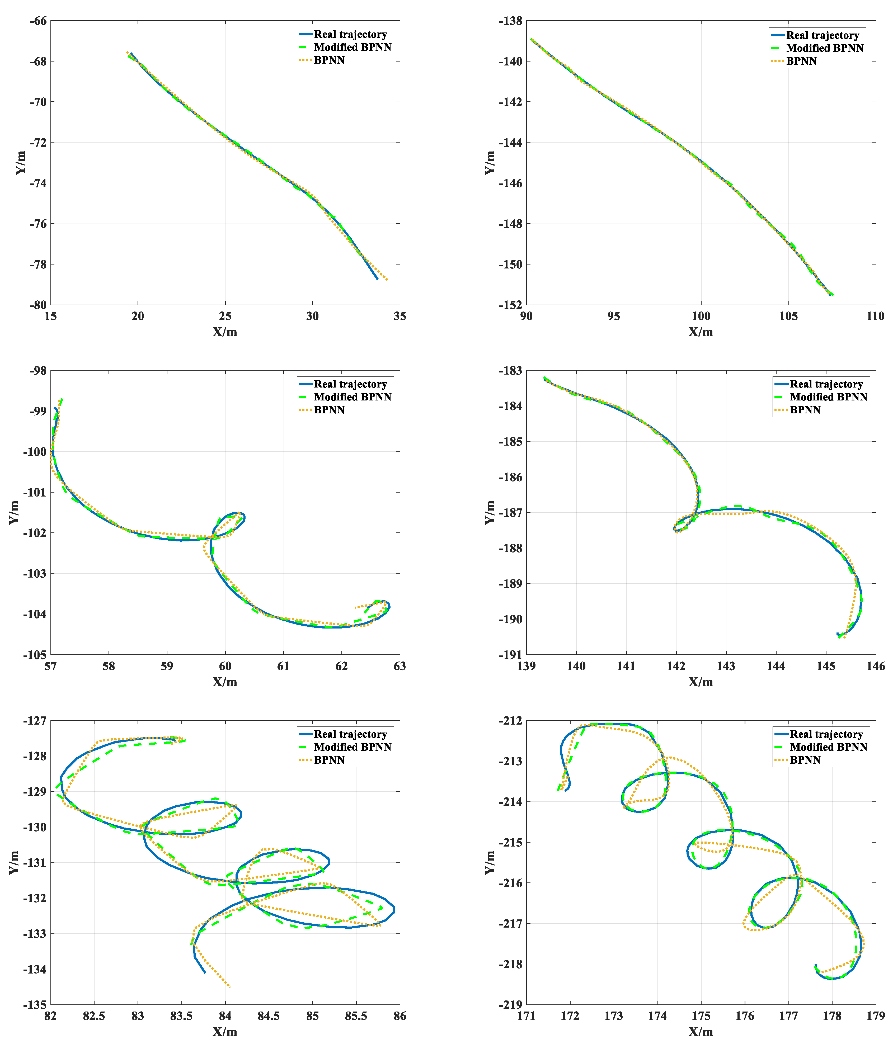
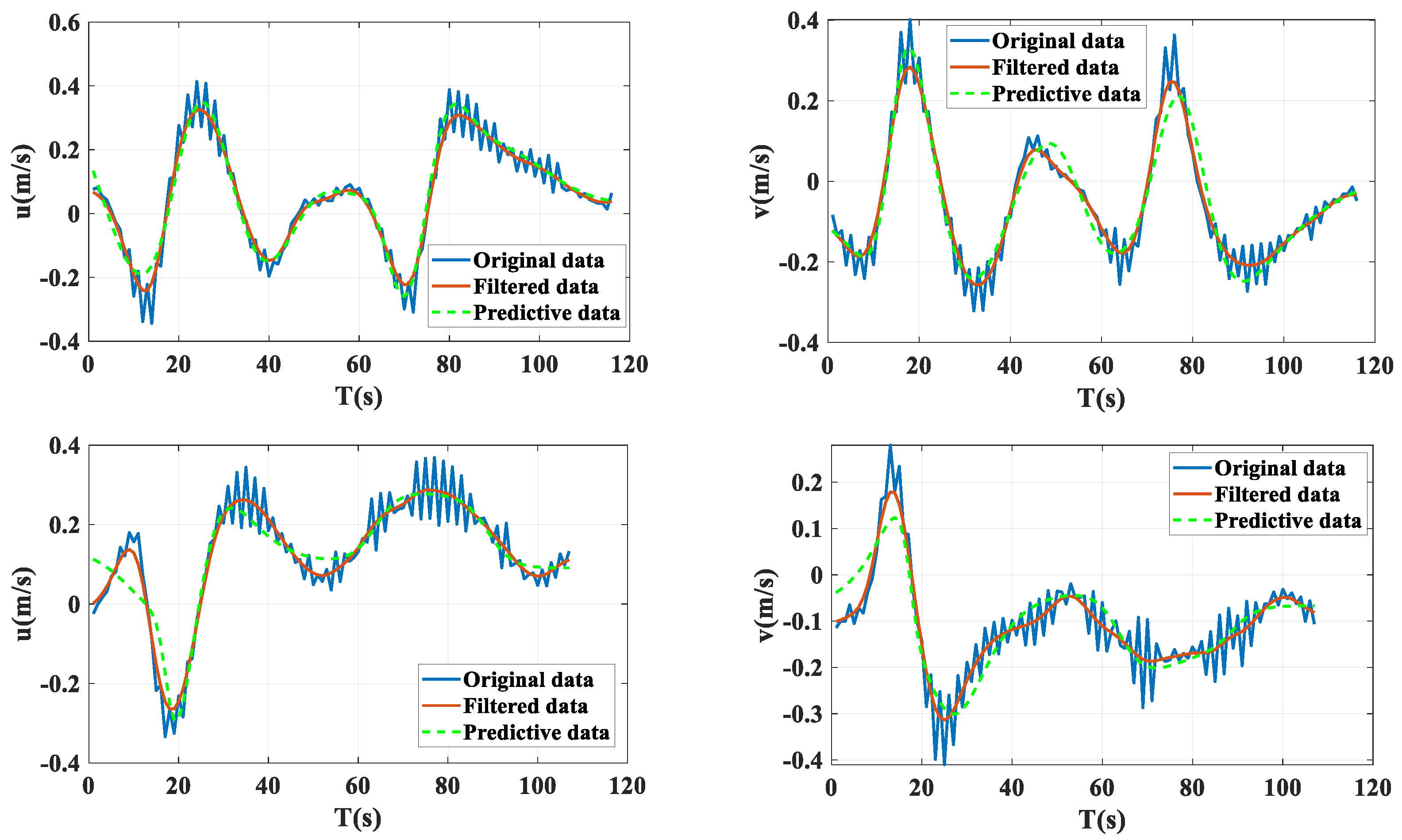
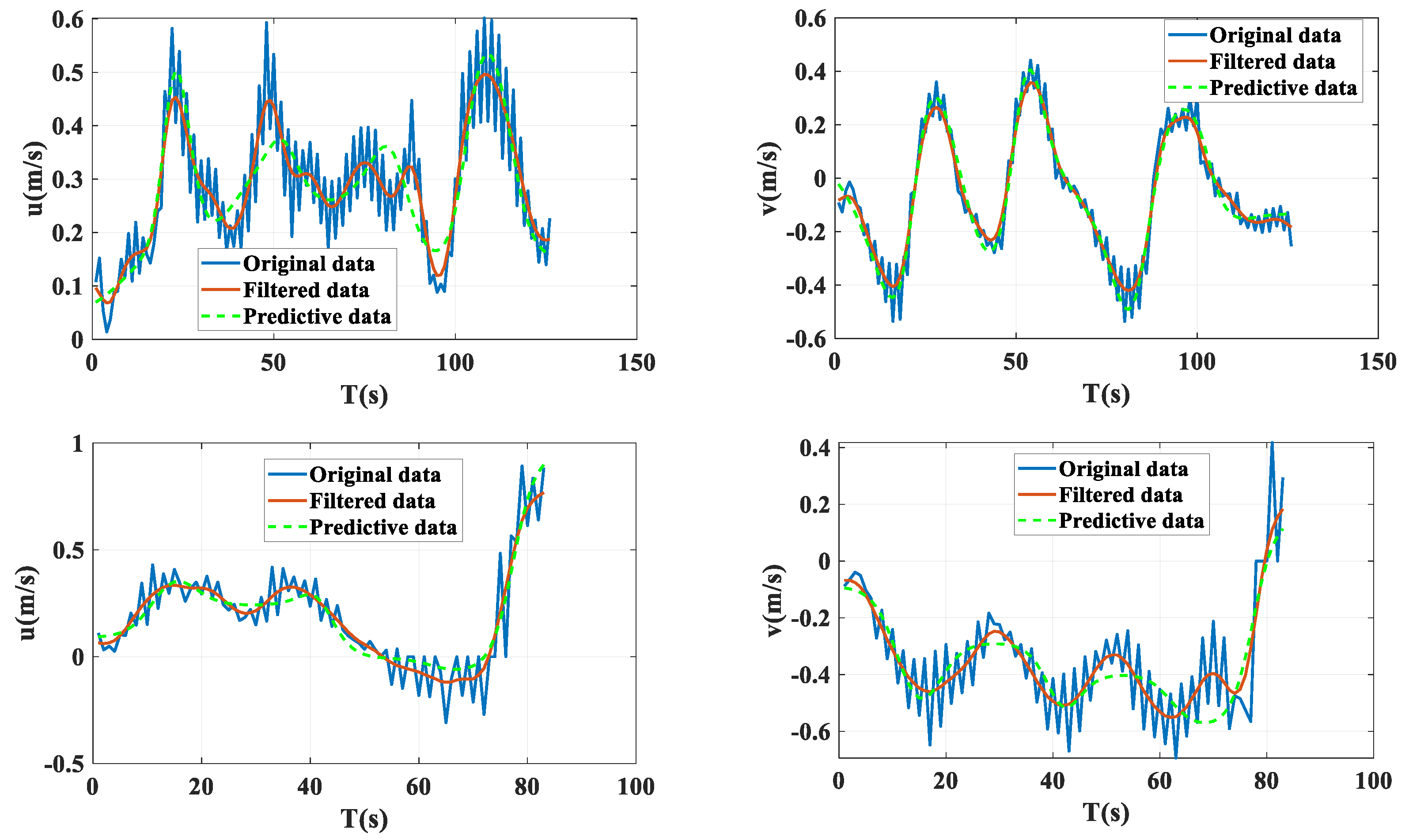
4. Experimental Setup and Simulation Results

In order to realize the experimental demonstration of the improved BPNN algorithm, we prepared a USV, which is equipped with a propeller that can feedback the speed. At the same time, it is also equipped with a wealth of sensors, including GPS, attitude sensors, electronic compass, and other sensors, which can provide us with track, heading Angle, speed, Roll, Pitch, Yaw, and other data. The USV ship is equipped with a radio communication radio, which can transmit these data to the shore control software at a frequency of 5 Hz in real time and can display and store the data in real time. The topological relationship of the ship control system is shown in Figure 6.
The investigation was carried out in Nanjing’s Qing-Huai River, as shown in Figure 7. It is worth noting that wind and current were consistently present at this particular site. Figure 8 displays the YL1300M expeditions throughout the Qing-Huai river. The turning experiments for the unmanned surface vehicle were conducted by varying the revolution speed of the propeller. The selection of distinct revolution speeds for the left and right propellers is evident in Table 1. Initially, the vehicle came to a halt on the water, utilizing the distinct revolutions per minute (RPM) of both the left and right propellers to push the YL1300M. This enabled the acquisition of rotation performance data under intricate circumstances. The neural network was trained using 70% of the available data, while the remaining 30% was reserved for testing purposes.
Figure 9 provides a visual representation of the YL1300M ‘s trajectory under varying propeller revolution speeds. The insightful depiction allows us to observe how the left and right propellers contribute to the vehicle’s movement at rotational speeds of 100 rpm, 500 rpm, and 1000 rpm. In the left column, a sequence of three images elucidates the trajectory of the left propeller, while the right column concurrently showcases the trajectory of the right propeller at the same rotational speeds. It becomes evident that the YL1300M‘s path deviates from the anticipated conventional circular trajectory. The images in the left column exhibit the subtle nuances in the trajectory as the propeller revolution speeds increase. At 100 rpm, the trajectory seems relatively stable, maintaining a certain symmetry. However, as the rotational speed escalates to 500 rpm and 1000 rpm, we begin to observe deviations in the circular path, hinting at the influence of external factors or system dynamics. Interestingly, the right column reveals a complementary set of images illustrating the trajectory under negative rotational speeds (−100 rpm, −500 rpm, and −1000 rpm). This adds a layer of complexity to the analysis, as negative rotational speeds might introduce counteracting forces, potentially affecting the overall stability and direction of the YL1300M. The visual representation in Figure 8 not only captures the expected circular trajectory but also unveils subtle deviations and nuances induced by varying propeller revolution speeds. This nuanced analysis provides valuable insights into the dynamic behavior of the YL1300M, shedding light on potential factors influencing its trajectory under different operational conditions.
Due to the influence of wind and current, the actual trajectory deviates from a circular path and instead takes the form of a linear or spiral trajectory. When the propellant’s velocity of rotation is low, the trajectory of the vehicle resembles a straight line. The lateral velocity is significantly smaller in comparison to the velocity of the current, resulting in the current exerting a dominant influence on the vehicle’s motion. Consequently, the ship moves in accordance with the current, leading to a linear trajectory. When the rotational velocity of the propeller reaches a high magnitude, the resulting path followed by the ship can be described as a spiral progression. The surge speeds and sway speeds exceed the magnitude of the current velocity, resulting in a ship’s motion characterized by a combination of circular trajectory and forward movement. Furthermore, the overall trajectory of the movement aligns with the direction of the current, as depicted in Figure 7. The predictive trajectory determined by the modified BPNN is represented by the blue dotted lines, while the traditional BPNN is represented by the yellow dotted lines. Table 2 demonstrates that the modified Backpropagation Neural Network (BPNN) has superior predictive capabilities for trajectory estimation compared to the conventional BPNN. This approach also exhibits a strong compatibility with the actual trajectory of the vehicle in the presence of wind and current. Furthermore, the modified backpropagation neural network (BPNN) exhibits a higher rate of convergence compared to the original BPNN. Hence, the utilization of the additional momentum method and adaptive learning rate method in enhancing the BPNN yields superior results in predicting the motion of vehicles. There are three types of track types in the experiment: smooth curve without turning, one turning circle, and multiple turning circles. After the experimental demonstration, BPNN can still predict more accurately in the first two working conditions, but when encountering multiple groups of rotation or the greater the curvature, BPNN will completely predict out of control. In contrast, the modified BPNN algorithm has better adaptability, and the effect is far superior to the traditional BPNN.
Figure 10 offers a comprehensive visualization of the interplay between empirical observations and predictive data, meticulously acquired through the sophisticated application of a refined Backpropagation Neural Network (BPNN) operating across a spectrum of propeller revolution speeds. The deliberate alignment of the six images in Figure 9 mirrors the arrangement in Figure 8, facilitating a detailed comparative analysis. The discernible rhythmic behavior captured in the data is a consequence of the inherent noise introduced during the meticulous process of data collection. In response to this challenge, the Gaussian filter technique emerges as a pivotal tool, systematically employed to mitigate and filter out noise from the dataset. The outcome is depicted graphically by the red line, unveiling a nuanced narrative delineated by two distinctive phases: acceleration and stability.
Within the intricate interplay of data and model predictions, it becomes evident that the forecasted data elegantly conforms to the intricate dynamics of both acceleration and stabilization stages. However, an analytical eye acknowledges a peak in the error rate, reaching a maximum of 11.33%. This nuanced observation underscores the inherent complexity of the system and hints at potential areas for refinement in the predictive modeling process. Nevertheless, the overall accuracy of the improved Backpropagation Neural Network (BPNN) in delineating the complete rotational speed process across the diverse spectrum of propeller revolution speeds remains notably high, showcasing the model’s capacity for capturing and interpreting the intricate dynamics of the propulsion system. The data and curves in Figure 9 and Figure 10 and Table 2 significantly show that the improved BPNN algorithm is relatively reliable in predicting different propeller speeds and track stability.
Transitioning to Figure 11, Figure 12 and Figure 13, these visual representations intricately dissect the surge velocities and sway velocities observed across varying propeller revolution speeds. The rhythmic patterns discernible in both surge and sway velocities are attributed to the intricate interplay of factors, intertwined with the rotational speed of the propeller. The meticulous projection of these patterns is encapsulated by the green dotted lines, serving as visual overlays that encapsulate the predicted values and patterns extrapolated from the empirical data obtained under distinct propeller revolution speeds. The analysis extends to the amplitude of the predicted values, revealing an admirable alignment with the actual observed values. The meticulous calibration of the predictive model is further emphasized by the recorded maximum inaccuracy rate of 8.9%. This attests to the model’s robustness, demonstrating a commendable efficacy in navigating the complexities of forecasting surge and sway velocities even under dynamically intricate conditions. The multifaceted analysis presented in Figure 10, Figure 11, Figure 12 and Figure 13 encapsulates the synergy between empirical data and predictive modeling, shedding light on the intricate dynamics of the propulsion system under varying operational conditions. The nuances observed in the rhythmic behavior and predictive accuracy offer valuable insights for future refinements, emphasizing the perpetual pursuit of precision and understanding in the realm of marine propulsion systems.

5. Conclusions

This study focused on the identification of a three-degree-of-freedom unmanned surface vehicle named YL1300M. Due to the influence of wind, ocean currents, and various unpredictable disruptions, researchers decided to employ a neural network in order to accurately discern and analyze the dynamics of ships. The Backpropagation Neural Network (BPNN) is a valuable approach for addressing complex nonlinear problems, while it does possess certain limitations. The traditional backpropagation neural network (BPNN) was enhanced by using the additional momentum method and the adaptive learning rate approach. Avoiding local minima is a challenging task that can enhance the convergence speed and precision of conventional Backpropagation Neural Networks (BPNNs). The findings indicate:
(1)
The modified BPNN exhibits enhanced convergence speed and superior ship trajectory prediction capabilities compared to the conventional BPNN. The calculated trajectories of the propeller at various rotational speeds exhibit a strong correlation with the actual trajectories.
(2)
The improved BPNN demonstrates effective estimation capabilities for the rotational velocity throughout both the acceleration and stability stages at various revolutions per minute (rpm) of the propeller. Furthermore, reliable predictions have been made for the acceleration of an increase and sway, in comparison to their actual values.
For the dynamic coefficient of the USV, the trajectory of the receiver and the main engine rotation speed are predicted by the improved BPNN algorithm. Compared with the traditional BNPP algorithm, the proposed algorithm has a larger lift, but still has a higher error when compared with the actual data of the real ship. By analysis, it is thought that there may be unreliable data when acquiring real-time data, or the weight allocation of the algorithm needs to be adjusted. Further studies could be made on this basis in the future. At the same time, the improved idea of this algorithm can be extended to other engineering fields, such as unmanned aerial vehicles, and inverted pendulums, especially in the scenes where the coefficients of nonlinear kinematic equations need to be recognized. The future identification algorithm based on data-driven dataless models will inevitably have more and wider applications.

Author Contributions

Conceptualization, S.Z.; Methodology, S.Z.; Validation, C.C.; Investigation, S.Z.; Data curation, C.C.; Writing—original draft, S.Z.; Writing—review & editing, G.L.; Supervision, G.L.; Project administration, S.Z. All authors have read and agreed to the published version of the manuscript.

Funding

This research received no external funding.

Institutional Review Board Statement

Not applicable.

Informed Consent Statement

Not applicable.

Data Availability Statement

Data are contained within the article.

Conflicts of Interest

The authors declare no conflict of interest.

References

  1. Gianluca, A.; Stefano, C.; Paolo, D.L. On data-driven identification: Is automatically discovering equations of motion from data a Chimera? Nonlinear Dyn. 2023, 111, 6487–6498. [Google Scholar] [CrossRef]
  2. Nagumo, J.I.; Noda, A. A learning method for system identification. IEEE Trans. Autom. Control 1967, 12, 282–287. [Google Scholar] [CrossRef]
  3. Holzhuter, T. Robust identification scheme in an adaptive track controller for ships. In Proceedings of the 3rd IFAC Symposium on Adaptive System in Control and Signal Processing, Glasgow, UK, 19–21 April 1989; pp. 118–123. [Google Scholar]
  4. Kallstrom, C.G.; Astrom, K.J. Experiences of system identification applied to ship steering. Automatica 1981, 17, 187–198. [Google Scholar] [CrossRef]
  5. Yoon, H.K.; Rhee, K.P. Identification of hydrodynamic coefficients in ship maneuvering equations of motion by estimation-before-modeling technique. Ocean Eng. 2003, 30, 2379–2404. [Google Scholar] [CrossRef]
  6. Shin, J.; Kwak, D.J.; Lee, Y.-I. Adaptive path following control for an unmanned surface vessel using an identified dynamic model. IEEE/ASME Trans. Mechatron. 2017, 22, 1143–1153. [Google Scholar] [CrossRef]
  7. Selvam, R.P.; Bhattacharyya, S.; Haddara, M. A frequency domain system identification method for linear ship maneuvering. Int. Shipbuild. Prog. 2005, 52, 5–27. [Google Scholar]
  8. Di Vito, D.; Cataldi, E.; Di Lillo, P.; Antonelli, G. Vehicle Adaptive Control for Underwater Intervention Including Thrusters Dynamics. In Proceedings of the 2018 IEEE Conference on Control Technology and Applications (CCTA), Copenhagen, Denmark, 21–24 August 2018; pp. 646–651. [Google Scholar]
  9. Rajesh, G.; Bhattacharyya, S. System identification for nonlinear maneuvering of large tankers using artificial neural network. Appl. Ocean Res. 2008, 30, 256–263. [Google Scholar] [CrossRef]
  10. Oskin, D.A.; Dyda, A.A.; Markin, V.E. Neural Network Identification of Marine Ship Dynamics. In Proceedings of the 9th IFAC Conference on Control Applications in Marine Systems, Osaka, Japan, 17–20 September 2013. [Google Scholar]
  11. Pan, C.Z.; Lai, X.Z.; Yang, S.X.; Wu, M. An efficient neural network approach to tracking control of an autonomous surface vehicle with unknown dynamics. Expert Syst. Appl. 2013, 40, 1629–1635. [Google Scholar] [CrossRef]
  12. Bibuli, M.; Zereik, E. Analysis of an unmanned underwater vehicle propulsion model for motion control. J. Guid. Control Dyn. 2022, 45. [Google Scholar] [CrossRef]
  13. Fossen, T.I. Marine Control Systems: Guidance, Navigation and Control of Ships, Rigs and Underwater Vehicles; Marine Cybernetics: Trondheim, Norway, 2002. [Google Scholar]
  14. Woo, T.; Park, J.Y.; Yu, C.; Kim, N. Dynamic model identification of unmanned surface vehicles using deep learning network. Appl. Ocean Res. 2018, 78, 123–133. [Google Scholar] [CrossRef]
  15. Sonnenburg, C.R.; Woolsey, C.A. Modeling, identification, and control of an unmanned surface vehicle. J. Field Rob. 2013, 30, 371–398. [Google Scholar] [CrossRef]
  16. Li, J.C.; Zhao, D.L.; Ge, B.F.; Yang, K.W.; Chen, Y.W. A link prediction method for heterogeneous networks based on BP neural network. Physica A 2017, 495, 1–17. [Google Scholar] [CrossRef]
  17. Hagan, M.T.; Menhaj, M.B. Training feedforward networks with the Marquardt algorithm. IEEE Trans. Neural Netw. 1994, 5, 989–993. [Google Scholar] [CrossRef] [PubMed]
  18. Suri, R.N.; Deodhare, D.; Nagabhushan, P. Parallel Levenberg_Marquardt-based neural network training on Linux clusters—A case study. In Proceedings of the Third Indian Conference on Computer Vision, Graphics & Image Processing, Ahmadabad, India, 16–18 December 2002. [Google Scholar]
Figure 1. The design of the YL1300M.
Jmse 12 00297 g001
Figure 2. A schematic representation of the USV’s differential thrust.
Jmse 12 00297 g002
Figure 3. A BP neural network.
Jmse 12 00297 g003
Figure 4. A neural unit.
Jmse 12 00297 g004
Figure 5. The procedure of mistake the gradient backpropagation for a unit.
Jmse 12 00297 g005
Figure 6. Topology diagram of USV control system.
Jmse 12 00297 g006
Figure 7. The Qing-huai river in google map.
Jmse 12 00297 g007
Figure 8. YL1300M expedition on the Qing-Huai River.
Jmse 12 00297 g008
Figure 9. The trajectory of the YL1300M.
Jmse 12 00297 g009
Figure 10. Real and estimated outputs of the different rotation speeds.
Jmse 12 00297 g010
Figure 11. The surge velocities and sway velocities in left propeller and right propeller at 100 rpm and −100 rpm.
Jmse 12 00297 g011
Figure 12. The surge velocities and sway velocities in the left propeller and right propeller are at 500 rpm and −500 rpm.
Jmse 12 00297 g012
Figure 13. The surge velocities and sway velocities in left propeller and right propeller are at 1000 rpm and −1000 rpm.
Jmse 12 00297 g013
Table 1. The different revolution speeds of the propeller were operated in experiments.
Left (RPM)Right (RPM)Left (RPM)Right (RPM)Left (RPM)Right (RPM)
−10000−100−100−100
−20000−200−200−200
−30000−300−300−300
−40000−400−400−400
−50000−500−500−500
−60000−600−600−600
−70000−700−700−700
−80000−800−800−800
−90000−900−900−900
−100000−1000−1000−1000
10000100100100
20000200200200
30000300300300
40000400400400
50000500500500
60000600600600
70000700700700
80000800800800
90000900900900
100000100010001000
Table 2. The standard deviation of error at different RPM.
100 RPM500 RPM1000 RPM
X (m)Y (m)X (m)Y (m)X (m)Y (m)
Traditional BPNN0.0550.0330.1390.1510.1470.325
Modified BPNN0.0480.0280.1210.1470.1330.287
−100 RPM−500 RPM−1000 RPM
X (m)Y (m)X (m)Y (m)X (m)Y (m)
Traditional BPNN0.0620.1030.1180.1030.1380.289
Modified BPNN0.0440.0880.1050.0960.1150.244
Disclaimer/Publisher’s Note: The statements, opinions and data contained in all publications are solely those of the individual author(s) and contributor(s) and not of MDPI and/or the editor(s). MDPI and/or the editor(s) disclaim responsibility for any injury to people or property resulting from any ideas, methods, instructions or products referred to in the content.

