Abstract
When we tested the water jet propulsion pump, we found that there were significant vibrations in the pump, especially at small flow points that deviated from the design conditions. The water jet propulsion pump is a mixed-flow pump with guide vane, which is commonly employed for water jet propulsion. However, the guide vane mixed-flow pump is susceptible to a phenomenon known as “hump”, which can cause flow disturbances, increased vibration, and noise when the pump operates within the hump region. According to the vibration phenomenon found in our experiment, the mechanism of vibration needs to be revealed. This study focuses on vorticity and turbulence distributions of a mixed flow water jet propulsion pump under the valley and peak operating conditions of the hump region. The research is conducted using experimental and numerical simulation methods. The SST k-ω turbulence model is employed for turbulence calculations. The experiments are conducted on a closed test rig for axial (mixed) flow pumps. A comparison of experimental and numerical simulation results of hydraulic performance curves are conducted to validate the accuracy of the numerical simulation. Cavitation flow structures of the critical cavitation stage under valley conditions and under peak conditions are compared. A comparative analysis is conducted to examine the differences in internal vortex core distribution and turbulence kinetic energy distribution between the valley and peak operating conditions when working within the hump region. The pressure and velocity vectors of the pump impeller blades and the velocity streamline distribution between the impeller and the guide vane blades are compared. To further analyze the flow state in different flow channels under valley and peak conditions, the streamline distribution at Span = 0.5 in the impeller and diffuser basin is extracted. This study provides theoretical foundations and technical support for the design of high-performance, low-vibration water jet propulsion pumps.
1. Introduction
A water jet propulsion pump is a type of pump used to generate propulsion for watercrafts. It works by drawing in water and then expelling it at a high velocity through a nozzle, creating a powerful jet that propels the vessel forward. This technology is commonly used in boats and ships, particularly in applications where high maneuverability and shallow-water operations are required. Water jet propulsion pumps have issues like lower efficiency compared to propeller-based systems, cavitation which can damage the impeller, high maintenance requirements, noise and vibrations, and reduced efficiency at high speeds [1]. Despite these issues, water jet propulsion pumps offer advantages in certain applications, such as increased maneuverability in shallow waters and a reduced risk of damage from submerged objects. Advances in design and technology continue to address the challenges associated with their operation.
As a rotating machine, the water jet propulsion pump has a very complex flow, and the flow in the flow channel between the blades is symmetrical in design. However, in practice, the flow in the flow channel between the blades is asymmetrical, especially the hump region operation condition.
Unlike the development of propeller propulsion that dates to the 19th century, water jet propulsion has emerged as a distinct propulsion method in the past 40 years. It utilizes the reactive force of the water jet expelled by the propulsion pump to propel the vessel forward. Compared to conventional propeller propulsion, water jet propulsion offers advantages such as low noise, excellent cavitation resistance, good maneuverability, and high propulsion efficiency at high speeds [2]. As a result, it has found increasingly widespread application in high-performance vessels. The water jet propulsion pump is responsible for the energy conversion function of the water jet propulsion system and is considered the core component of the system. Due to installation and layout constraints, axial-flow pumps or guide-vane mixed-flow pumps are commonly selected for water jet propulsion pumps [3,4,5,6]. However, high-specific-speed mixed-flow pumps and axial-flow pumps tend to exhibit humps or even double humps in their flow-head characteristic curves. When the pump operates within the hump region, flow disturbances, increased vibration, and noise may occur throughout the pump and the entire system. During the variable-speed navigation of the vessel, the water jet propulsion pump needs to undergo corresponding speed changes. However, the pump may enter the hump region during speed variation, which is detrimental to the efficient and low-noise operation of the vessel, affecting the comfort of the crew and the stealth of military vessels, and even causing damage to the propulsion system.
The abnormal phenomenon of a turning point on the pump head flow (flow coefficient QnD and energy coefficient EnD) curve, as shown in Figure 1, is referred to as the pump hump phenomenon. The region where the hump phenomenon occurs is known as the hump region or saddle region, according to some scholars. Currently, scholars worldwide generally agree that the hump phenomenon originates from changes in the flow state within the pump. However, there are two main viewpoints regarding the direct cause of the hump phenomenon. One viewpoint suggests that the changes in the flow state within the pump result in non-monotonic variations in hydraulic losses, leading to the occurrence of the hump phenomenon. The other viewpoint proposes that the changes in the flow state within the pump cause variations in the impeller’s functional capacity, resulting in the hump phenomenon.
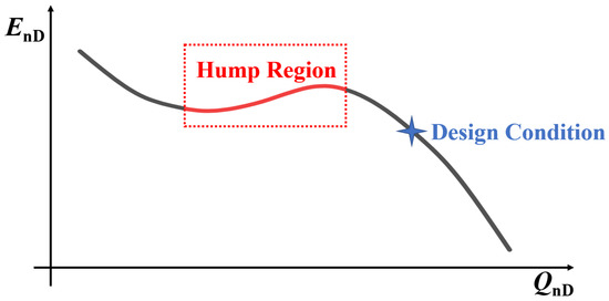
Figure 1.
Diagram of pump performance curve hump phenomenon.
For centrifugal pumps, the stability of their performance is related to the rising slope of the flow-head curve [7]. The larger the absolute value of this slope, the more stable the actual performance curve. When the pump is working within the hump region, the amplitude of low-frequency signal increases as a result of this [8]. Liu Yong [9] attributed the hump phenomenon in centrifugal pumps primarily to the reduction in impeller’s functional capacity due to rotational stall, followed by the increased asymmetry of the flow and turbulence intensity within the volute, resulting in increased hydraulic losses. The theoretical head-flow curve of centrifugal pumps is more prone to exhibit humps, and the selection of an appropriate blade outlet angle and blade profile curvature helps to address the hump problem in pumps [10,11,12].
Regarding mixed-flow pumps, Li Wei [13] and Li Enda [14] believe that the hump phenomenon in guide-vane mixed-flow water jet propulsion pumps is the result of a combination of factors such as rotational stall, leading edge flow separation, and trailing edge backflow. Weixiang Ye [15] identified a significant increase in energy losses in the impeller of mixed-flow pumps as the primary cause of the hump phenomenon, with a notable decrease in blade loading near the leading edge, ultimately resulting in reduced head.
For mixed-flow water pump turbines, Li Qifei [16] proposed that as the flow rate decreases, the axial velocity decreases, the incidence angle increases, and flow separation and the vortex phenomena occur on the suction surface, resulting in a blockage in the flow passage, increased energy losses, and reduced head. This leads to the formation of a valley point on the flow-head curve, ultimately resulting in the hump phenomenon. Yang Jun, G. Pavesi, Uroš Ješe, O. Braun, and others [17,18,19,20,21] attributed the hump phenomenon in pump-turbines under pump operation to the influence of the dynamic–stator interaction on the flow structure and pressure pulsation inside the runner outlet and adjustable guide vanes.
Liu Yong [22] proposed a new method based on the second-order derivative of external characteristics to characterize the energy coefficient. By quantitatively expressing the working capacity of the runner and the hydraulic losses of various hydraulic components, the key factors triggering the hump phenomenon can be determined. It suggests that the direct cause of the hump formation is the non-monotonic decrease in the runner’s functional capacity, where the blockage and pressure increase effect of the stalled vortex in the movable guide vanes affect the runner’s functional capacity, thereby inducing the hump phenomenon. Li Deyou and Chen Jinxia [23,24] suggested that the humps near the optimal operating conditions are mainly due to increased hydraulic losses, while the humps away from the optimal operating conditions are attributed to the decrease in Euler’s energy and the increase in hydraulic losses. The hysteresis effect of the hump phenomenon is caused by the different hydraulic losses and Euler’s energy in the directions of the decreasing and increasing flow rates, with hydraulic losses playing a dominant role.
In summary, many scholars have conducted extensive research on various types of pumps such as centrifugal pumps, mixed-flow pumps, axial-flow pumps, and pump turbines to understand the causes of the hump phenomenon. However, different viewpoints have emerged regarding the different types of pumps, and there is no consensus on the cause of the hump. Furthermore, there is relatively limited research on the mixed-flow water jet propulsion pump with the diffuser.
The current research on the complex flow structure of the water jet pump mainly includes several directions such as flow in the hump region, non-uniform inflow conditions, cavitation flow, and transient start-stop conditions, and has made many progresses. However, there are few studies on vorticity and cavitation flow in the hump region. In this paper, based on the hump phenomenon found in the experiments, the inner flow distribution and cavitation flow structure in the hump region of the water jet propulsion pump is studied and analyzed.
2. Experimental Model and Test Platform
2.1. Experimental Pump Structure and Parameters
In this experiment, a mixed-flow pump with a contraction vane is selected as the research object. The model pump’s main parameters are shown in Table 1. The hydraulic components of the model pump include the suction pipe, impeller, diffuser, pump shaft, and out pipe, as shown in Figure 2.

Table 1.
Design parameters of the experimental pump.
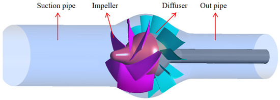
Figure 2.
The hydraulic components.
2.2. Test Platform and Method
2.2.1. Experimental Testing Method and Apparatus
The experiments were conducted on the closed test bench for axial or mixed flow pumps at National Research Center of Pumps in Jiangsu University. The test focused on hydraulic performance, cavitation performance, and the high-speed photography of the model pump. Experimental data acquisition was performed using the pump product testing system. The measured accuracy of the system was 0.2% for power, 0.02% for flow rate, and 0.02% for pressure measurement.
2.2.2. Experimental Principles and Methods
The hydraulic performance test of the model pump was conducted according to the national standard GB/T 3216-2016 [25]. The cavitation performance test was conducted according to the national standard GB/T 13006-2013 [26]. Pressure measurements were performed using pressure transmitters that convert pressure signals into current signals, which were then transmitted to the pump parameter measurement instrument.
A 3D model of experimental pump is shown in Figure 3a. Prior to starting the experiment, the test pipeline was connected according to Figure 3b. The impeller was made of a copper alloy. The diffuser was made of stainless steel. The torque meter was zero-calibrated under no-load conditions before filling the pipeline with water to eliminate mechanical losses caused by bearings and sealing components. As the test pump is a mixed-flow pump, it is started by opening the valve. The direct current variable frequency motor was adjusted to the test speed, and once the operation stabilized, the valve opening was adjusted to control the flow rate. Data were collected to complete the hydraulic performance test.
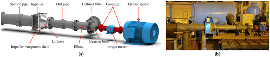
Figure 3.
Experimental loop and the model pump. (a) 3D model of experimental pump; (b) experimental loop.
3. Numerical Simulation Method
3.1. Grid Generation
TurboGrid was used to generate hexahedral structured grids for the impeller and diffuser domain. Long straight pipe sections were added at the inlet of the impeller and the outlet of the diffuser. ICEM CFD was used for the hexahedral structured grid generation. The computational grids for hydraulic components are shown in Figure 4.
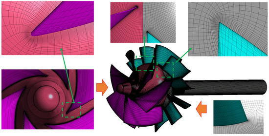
Figure 4.
Computational grid of hydraulic components.
3.2. Calculation Setting
3.2.1. Governing Equations
The commercial software ANSYS CFX 2021 R1 was used for the hydraulic performance calculations of the model pump. The liquid phase was assumed to be water at 25 °C, and the default material properties from the software’s database were used. The SST k-ω turbulence model was employed for turbulence calculations.
In the numerical simulation process of this paper, the fluid medium was incompressible viscous water. Because the temperature of the pump in the working process was almost unchanged, the calculation ignored the influence of heat transfer and heat exchange, and the control equation is expressed as follows:
- (1)
- Continuity equation
The mathematical expression in a Cartesian coordinate system is as follows:
where t is time, s; u is the velocity component of the fluid in the x direction, m/s; v is the velocity component of the fluid in the y direction, m/s; and w is the velocity component of the fluid in the z direction, m/s.
- (2)
- Momentum conservation equation
The mathematical expression for the momentum conservation equation is as follows:
where μ is the dynamic viscosity; τxx, τxy, and τxz, are the components of the viscous force τ acting on the surface of the micro-unit; and Fx, Fy, and Fz are the components of the volume force in three directions.
- (3)
- Turbulence model functions
In 1994, Menter proposed the SST model [27,28,29]. The SST model is accurate when calculating viscous flow in the near-wall region and when calculating far-field free flow, and in the mixed region, the two models are combined by a weighted function F1. The functions are as follows:
where y is the distance to the nearest wall, and ν is the kinematic viscosity. Furthermore, where γ = 5/9, β′ = 0.09, β = 0.075, σk = 0.5, σω = 0.5, and σω2 = 0.856. Gk is the term representing the generation of turbulent kinetic energy k. For free shear flow with unsuitable assumptions, F2 is used to constrain the limit number of wall layers, and F2 is a mixture function similar to Fl, which restricts the limiter to the wall boundary layer, as the underlying assumptions are not correct for free shear flows. S is an invariant measure of the strain rate.
3.2.2. Turbulence Model
It is very important to select the appropriate turbulence model for numerical calculations. In order to obtain the energy characteristic curve, which is more similar to the experimental curve, four different turbulence models, namely the standard k-ε model, RNG k-ε model, standard k-ω model, and SST k-ω model, which are commonly used in practical engineering, were selected for the comparison of the preliminary numerical simulations.
In the direction of increasing flow, five flow conditions, QnD = 0.0063, QnD = 0.0087, QnD = 0.0122, QnD = 0.0151, and QnD = 0.0181 (corresponding to 0.32Qd, 0.44Qd, 0.62Qd, 0.76Qd, and 0.92Qd, respectively) are selected for the numerical simulation and experimental verification. In the numerical calculation, only the turbulence model is different, and the other settings are consistent.
The head, torque, and efficiency data obtained by the numerical calculation of different turbulence models were dimensionless and transformed according to International Standard Committee (IEC) standards, and the results are shown in Figure 5. From the figure, it can be seen that the selected four turbulence models had basically the same change trend under the four flow conditions. The overall deviation of the k-ω model was small, and the deviation of the RNG k-ε model was large. However, only the SST k-ω model shows the same downward trend as the experimental energy coefficient EnD under the flow condition of QnD = 0.0181, although the decline was small. The SST k-ω model was deemed suitable for the water jet propulsion pump as it exhibited significant flow separation and backflow in the hump region under low flow conditions. Therefore, after comprehensive consideration, the SST k-ω model was adopted for numerical calculation in this paper.
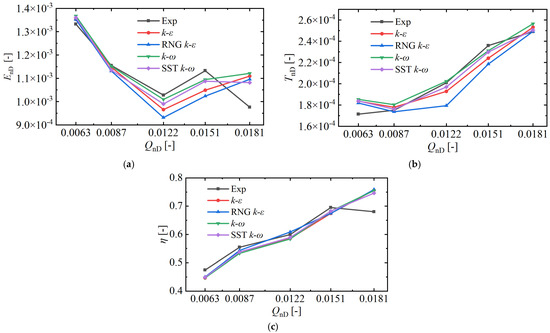
Figure 5.
Comparison of CFD results with different turbulence models and experiment. (a) Energy efficiency; (b) torque coefficient; (c) efficiency.
3.2.3. Boundary Conditions
The fluid domain of the impeller was defined as a rotating domain. The other fluid domains were set as stationary domains. The rotation was set as 750 r/min. The reference pressure was set as 0 Pa. The inlet boundary condition was set as the total pressure. The outlet boundary condition is set as mass flow rate, which is related to the operating condition.
For the wall boundary conditions, a no-slip wall condition was applied. The impeller blades, impeller hub, diversion cap, and shaft were defined as rotating walls, with the rotational speed matching the impeller speed. The impeller shroud was defined as a reverse rotating wall, while the remaining walls were set as stationary walls.
The interface between rotating and stationary components was defined as a frozen rotor interface. The advection scheme option was set to high resolution. The difference scheme was selected as first order upwind. The maximum number of iteration steps was 1000 steps. The convergence criterion was set as 10−4 for residual values. We selected the results of the calculating step whose convergence residual was reach to 10−4 for analysis.
3.3. Grid Independence Verification
To ensure grid independence, five sets of grid schemes were generated by adjusting the grid density while maintaining the topology and the first layer height near the walls. The number of grid cells for each component and the corresponding calculation results are shown in Figure 6. In the figure, the abscissa shows the five schemes, the left vertical coordinate shows the number of meshes of different hydraulic components of each scheme, and the right coordinates are the energy coefficient EnD, torque coefficient TnD, and efficiency η. From the figure, it can be observed that as the grid was refined, the energy coefficient EnD, torque coefficient TnD, and efficiency η tended to stabilize. Scheme 4 and Scheme 5 yielded nearly identical results. However, to capture the finer flow field structures as much as possible, Scheme 5 was chosen for the final calculation. It consisted of a total of 12.54 million cells, with 1.74 million cells for the inlet pipe, 4.09 million cells for the impeller, 5.42 million cells for the diffuser, and 1.29 million cells for the outlet pipe.
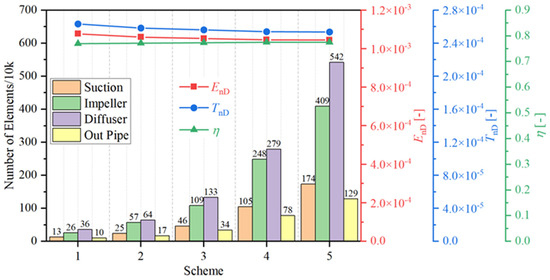
Figure 6.
Composition of grid numbers for different schemes and its computational results.
4. Results and Analysis
To enhance the universality of the experimental and numerical results, the flow rate Q, head H, and impeller torque T data obtained from the experiments and simulations were made non-dimensional according to the International Electrotechnical Commission (IEC) standards using the following equations:
In the equations, the flow coefficient QnD, energy coefficient EnD, and torque coefficient TnD are all dimensionless. The flow rate Q is in m3/s; rotational speed n is in rev/min; impeller nominal diameter D is in m; head H is in m; gravitational acceleration g is in m/s2; density ρ is in kg/m3; and torque T is in N·m.
4.1. Comparison of Experimental and Numerical Simulation Results of Hydraulic Performance Curves
The numerical simulation results are non-dimensional and compared with the experimental data to validate the accuracy of the numerical simulation. The comparative results are shown in Figure 7. The abscissa shows the flow coefficient QnD, the left vertical coordinate shows the energy coefficient EnD, and the right vertical coordinates represent the torque coefficient TnD and efficiency η.
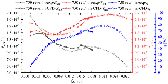
Figure 7.
Comparison of experimental and numerical simulation results of hydraulic performance curves.
From Figure 7, it can be observed that when the flow coefficient QnD is less than 0.004, the energy coefficient EnD obtained from the numerical simulation shows a significant deviation. However, for the remaining flow conditions, the deviations are relatively small, and there is a high degree of overlap in the hump region. The trend of the torque coefficient obtained from the numerical simulation is consistent with that obtained from the experiments. Additionally, the efficiency obtained from the numerical simulation is generally comparable to the experimental efficiency.
4.2. Cavitation Flow Structure of Water Jet Propulsion Pump under Hump–Peak–Valley Condition
The main difference between the cavitation flow of the model pump under the valley and peak conditions is that the tip leakage vortex obviously exists under the peak condition. The tip leakage vortex is usually caused by the pressure difference between the pressure surface and the suction surface, and the tip leakage vortex under the peak condition mainly exists in the tip front end. At the same cavitation development stage, the cavitation size in the pump under the peak condition is slightly larger than that under the valley condition.
The i-SPEED 3 high-speed camera from the British brand IX Cameras was used to capture the position and morphological evolution of cavitation inside impellers.
In order to observe the cavitation flow pattern of the water jet propulsion pump impeller, the impeller casing was made of organic glass material. To reduce image distortion caused by light refraction, the impeller casing was designed with an inner circular and outer square shape. During the shooting, the camera should be adjusted to be perpendicular to the shooting area, i.e., the camera’s vertical axis is perpendicular to the impeller’s axial plane. For ease of arrangement and adjustment, both should be placed at the same height, i.e., the impeller’s axial line and the camera’s axis line should be on the same horizontal plane, and the camera should be shooting from the side. The layout scheme of the test bench is shown in Figure 3.
According to the lighting conditions of the test site and the requirement for image clarity, combined with the functional parameters of the i-SPEED 3 high-speed camera, the shooting frame rate of the high-speed camera for this experiment was finally determined to be 2000 fps, corresponding to an image resolution of 1280 × 1024.
The shooting angle α for capturing the cavitation flow of the test pump, with the impeller rotating speed n and shooting frequency f, was calculated as
where α represents the impeller rotation angle (°), and n represents the impeller rotating speed (r/min). In this experiment, only the cavitation flow structure at a test speed of 1200 r/min is captured. The high-speed camera had a frame rate of 2000 fps, which means that a photo was taken every 3.6° of impeller rotation.
As shown in Figure 8a, in the critical cavitation stage of the near-valley condition, there are mainly vortex cavitation, cloud cavitation, vertical cavitation vortex, and other cavitation forms in the flow channel. LE and TE are the leading edge and trailing edge. SS is the suction surface and PS is the pressure surface. Cloud cavitation occurs at the suction side of the impeller blade near the leading edge. As the impeller rotates, grows, and gradually falls off, the shedding cloud cavitation gradually shifts downstream and is accompanied by the rotation of the cavitation vortex. The size of the hole between different flow channels is different. In the two adjacent channels, one channel is almost completely blocked by the hole, and the other channel is blocked by about 1/3 in the circumferential direction. At this time, the head of the test pump under this flow condition is about 3% lower than that under the initial condition. As shown in Figure 8b, in the critical cavitation stage of the near-peak conditions, there are mainly vortex cavitation, tip leakage vortex, cloud cavitation, vertical cavitation vortex, and other cavitation forms in the flow channel. Cloud cavitation occurs at the position where the suction surface of the impeller blade is close to the inlet edge. As the impeller rotates, the shedding cloud cavitation gradually shifts downstream and is accompanied by the rotation of the cavitation vortex. From the experimental observation, it is found that with the development of cavitation, the cavity size in the flow channel in the critical cavitation stage increases continuously. However, the hole size between different channels is still very different. In the two adjacent channels, one channel is almost completely blocked by holes, and the other channel is about half blocked in the circumferential direction. At this time, the head of the test pump under this flow condition is 3% lower than that under the initial condition.
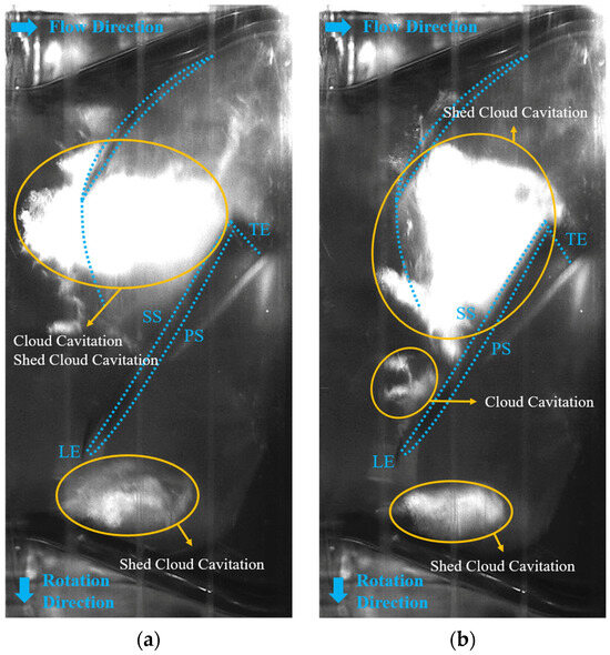
Figure 8.
Cavitation flow structures of critical cavitation stage under valley and peak conditions. (a) Valley condition; (b) peak condition.
4.3. Entropy Generation Distribution
To investigate the flow loss characteristics of the energy characteristic curve of the water jet propulsion pump under valley and peak flow conditions, a comparative analysis is performed using two flow conditions: valley and peak. Table 2 provides the distribution of entropy generation in different flow regions, where the entropy generation ratio represents the proportion of entropy generation in a specific fluid domain to the total entropy generation. From Table 2, it can be observed that compared to the valley flow condition, the entropy generation values within the inlet pipe and outlet pipe regions increased, while the entropy generation values within the impeller and diffuser regions decreased, resulting in a decrease in total entropy generation for the peak flow condition. Under the valley flow condition, entropy generation mainly occurred within the impeller, diffuser, and outlet pipe regions, with the diffuser region accounting for the largest proportion at 39.6%. Under the peak flow condition, entropy generation also predominantly occurred within the impeller, diffuser, and outlet pipe regions. However, the proportion of entropy generation within the impeller and diffuser regions decreased, while the proportion within the outlet pipe region increased and became the largest at 36.3%. In summary, the energy dissipation within the pump under valley and peak flow conditions mainly originates from the impeller, diffuser, and outlet pipe regions. Further analyses will be conducted to examine the energy dissipation components within the impeller, diffuser, and outlet pipe regions.
Table 2.
Entropy generation distribution in different flow domains.
Table 3, Table 4 and Table 5 present the composition of different forms of energy dissipation within the impeller, diffuser, and outlet pipe regions, respectively. From the tables, it can be observed that for both valley and peak flow conditions, the energy dissipation within the impeller, diffuser, and outlet pipe regions is primarily attributed to turbulent dissipation, followed by wall dissipation, while direct dissipation accounts for a very small proportion, not exceeding 1%. Under the valley flow condition, both the turbulent dissipation entropy generation value and proportion within the impeller, diffuser, and outlet pipe regions are higher compared to the peak flow condition. Specifically, within the impeller region, the proportion of turbulent dissipation entropy generation reaches 84.7%. This may be due to the larger turbulent structures and intensity within the pump under the valley flow condition. Under the peak flow condition, both the turbulent dissipation entropy generation value and proportion within the impeller and diffuser regions decrease, possibly due to reduced turbulent structures and intensity within the pump. Additionally, due to increased flow rate and velocity within the pump, the wall dissipation entropy generation value and proportion increase.
Table 3.
Composition of entropy generation in the impeller flow domain.
Table 4.
Composition of entropy generation in the diffuser flow domain.
Table 5.
Composition of entropy generation in the out pipe flow domain.
In conclusion, the energy dissipation entropy generation within the pump under valley and peak flow conditions mainly originates from the impeller, diffuser, and outlet pipe regions, with turbulent dissipation accounting for the highest proportion. Compared to the peak flow condition, the valley flow condition exhibits higher values and proportions of turbulent dissipation entropy generation within the impeller and diffuser regions.
4.4. Vorticity and Turbulence Distributions
The intensity of turbulent dissipation is closely related to the intensity of vortex structures. The Ω method [30] is used to extract the internal vortex structures within the pump under valley and peak flow conditions. Figure 9, Figure 10 and Figure 11 show the distribution of vortex cores within the impeller, diffuser, and out pipe, respectively.
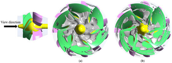
Figure 9.
Distribution of vortex cores inside the impeller under valley and peak conditions. (a) Valley condition; (b) peak condition.
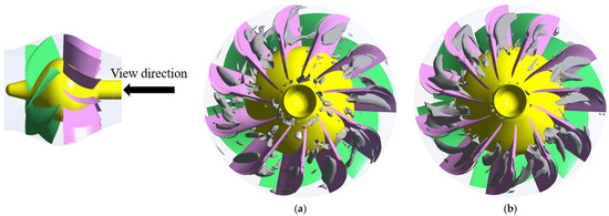
Figure 10.
Distribution of vortex cores inside the diffuser under valley and peak conditions. (a) Valley condition; (b) peak condition.
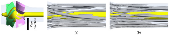
Figure 11.
Distribution of vortex cores inside the out pipe under valley and peak conditions. (a) Valley condition; (b) peak condition.
From Figure 9, compared to the peak condition, it can be observed that the valley operating condition exhibits a higher intensity of vortex cores near the hub region within the impeller. The intensity of the vortex cores near the shroud region in valley condition is higher. This means that in valley conditions, there is a large amount of energy dissipation in the impeller, resulting in a decrease in pump performance.
From Figure 10, compared to the peak condition, there are many more small-scale vortex cores near the diffuser hub region in the valley condition. However, there are obvious differences in the scale and strength of vortex structures between impeller flow channels. The scale of vortex structures present in the peak condition is larger.
From Figure 11, compared to the peak flow condition, the size of the vortex in the out pipeline of the valley condition is larger and more coherent. Under the peak condition, some large-scale vortices appear broken and reshaped.
Turbulent kinetic energy (TKE) is a physical quantity that characterizes the turbulent fluctuation intensity of the fluid, which is related to velocity fluctuation and turbulent dissipation. Its expression is as follows:
where u is the average velocity, m/s; and l is the turbulence intensity. The turbulent kinetic energy is proportional to the average velocity and turbulence intensity. The larger the value of turbulent kinetic energy, the more severe the energy dissipation of the fluid.
Figure 12 shows the distribution of turbulent kinetic energy within the pump under valley and peak flow conditions. The figure is based on a blade-to-blade view at different circumferential heights (from hub to shroud, Span = 0.1, 0.3, 0.5, 0.7, 0.9) within the impeller and diffuser. From the figure, it can be observed that the regions with high turbulent kinetic energy within the impeller region are mainly located near the shroud under both valley and peak flow conditions. Within the diffuser region, there are regions with high turbulent kinetic energy at different circumferential heights, but the distribution patterns vary. As the circumferential height increases, the turbulent kinetic energy at the inlet of the diffuser increases, while it decreases at the outlet.
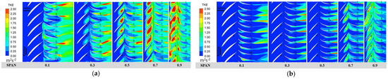
Figure 12.
Distribution of turbulence kinetic energy inside the pump under valley and peak conditions. (a) Valley condition; (b) peak condition.
Additionally, under the valley flow condition, there are regions with high turbulent kinetic energy near the hub within the clearance between the impeller and diffuser. This indicates a higher turbulent intensity in that region. Overall, under the valley flow condition, the impeller and diffuser regions exhibit higher turbulent kinetic energy compared to when under the peak flow condition. The regions with high turbulent kinetic energy align well with the regions with high entropy production, indicating that the entropy production within the pump is mainly composed of turbulent dissipation.
4.5. Pressure and Velocity Distributions
From Figure 13, it can be seen that under the valley condition, the streamline of the pressure surface of the impeller blade is also relatively smooth and uniform overall, and there is a small local backflow near the leading edge of the blade at the top of the blade. However, there are flow structures such as flow separation and vortex on the suction surface with a large spanwise height (as shown in the right block of Figure 13a), and the flow on different blades is quite different; particularly, the distribution of vortices on the suction surface on each blade is not uniform. Under the peak condition, the streamlines of the pressure surface and the suction surface of the impeller blade are relatively smooth and uniform, and the streamlines of the pressure surface appear to converge from the root to the trailing edge of the blade tip. The suction surface is close to the leading edge and the tip of the blade, and there is an obvious low pressure zone. At the same time, the range of the low pressure zone is not uniform on each blade, and the low pressure zone of one blade is not obvious.
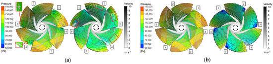
Figure 13.
Pressure and streamline distribution of impeller blades under valley and peak conditions. (a) Valley condition; (b) peak condition.
To further analyze the flow state in different flow channels under valley and peak conditions, the streamline distribution at a height of 0.5 in the impeller and guide vane basin was extracted (as shown in Figure 14). It can be seen from Figure 14a that there are large-scale backflow vortices and flow separation in the impeller and diffuser under the valley condition. The flow distribution in the impeller mainly appears at the trailing edge of the suction surface, the scale of the vortex structure in the six flow channels is not evenly distributed, and the vortex structure in each flow channel is quite different. Similarly, the scale of the vortex structure in the 11 flow channels in the diffuser is not evenly distributed, and the vortex structure in each flow channel is quite different. The vortex structure scale on the back of the sixth, eighth and tenth blades of the diffuser is more obvious. The vortex structure on the back of the eighth blade is particularly special, and there are three groups of vortices, which disturb each other. The vortex in the diffuser channel, especially the vortex at the inlet of the diffuser, also has an obvious influence on the flow in the impeller. From Figure 14b, it can be seen that under the peak condition, the streamlines of the impeller and the diffuser at the spanwise of 0.5 are smooth and uniform, and the flow is regular. Only a small backflow vortex appears on the back of the diffuser.
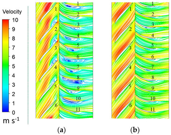
Figure 14.
Streamline distribution of inside the pump under valley and peak operating conditions (Span = 0.5). (a) Valley condition; (b) peak condition.
4.6. Discussion
The flow loss in the pump under valley and peak conditions mainly occurs in the impeller, diffuser, and outlet pipe basin, but the loss in diffuser basin accounts for the largest proportion under the valley condition and the largest proportion of outlet pipe basin under the peak condition. Flow losses in impeller, diffusers and outlet pipe basins under valley and peak conditions are mainly due to turbulent dissipation losses, followed by wall dissipation losses. In the valley condition, there is a large-scale reflux vortex and flow separation inside the impeller and diffuser. As the spreading height increases, the reflux vortex and flow separation gradually shift from the diffuser to the impeller. From the distribution of turbulent kinetic energy, when the pump is running in the hump valley, there is significant turbulent energy dissipation in the impeller and diffuser flow channel. From the slight differences, it can be found that there are obvious differences and asymmetries in the flow channels of different blades, among which the flow asymmetry in the diffusers is more prominent when Span = 0.1. When Span is in the range of 0.5~0.7, there is a more obvious flow asymmetry in the impeller, and the turbulence of some flow channels is stronger, while some are weaker. The correlation between these flow asymmetries and the vortex structure in the pump, as well as the flow excitation properties they induce, are complex. Subsequently, attention should be paid to the role of the flow angle and the leading edge of the blade in the pump under the valley and peak conditions, especially whether there is a phenomenon such as rotational stall, and whether the mechanism of flow-induced vibration should be solved from the flow perspective.
5. Conclusions
Here, we summarize the more complex discussion above. We have come to the following conclusions:
- (1)
- When we tested the water jet propulsion pump, we found significant vibrations in the pump, especially at small flow points that deviated from the design conditions. The performance curve of the pump was obtained by experimentation. A pronounced hump was found. According to the vibration phenomenon found in our experiment, the mechanism of vibration needs to be revealed.
- (2)
- Compared to the peak flow condition, the valley flow condition exhibits a higher intensity of vortex cores near the hub region within the impeller. The valley flow condition also has a greater number of small-scale vortex cores near the hub region within the diffuser. The intensity of vortex cores near the shroud region is approximately the same, but the overall intensity is higher. The valley flow condition has a lower overall intensity of vortex cores within the outlet pipe.
- (3)
- The regions with high turbulent kinetic energy in the impeller region are mainly located near the shroud under both valley and peak flow conditions. In the diffuser region, there are regions with high turbulent kinetic energy at different circumferential heights, but the distribution patterns vary. As the circumferential height increases, the turbulent kinetic energy at the inlet of the diffuser increases, while it decreases at the outlet. Additionally, during the valley flow condition, there are regions with high turbulent kinetic energy near the hub within the clearance between the impeller and diffuser. This indicates a higher turbulent intensity in that region. Overall, under the valley flow condition, the impeller and diffuser regions exhibit higher turbulent kinetic energy compared to when under the peak flow condition.
- (4)
- Comparing with the valley and peak pressure and velocity distributions shows that in the valley condition, the streamline of the pressure surface of the impeller blade is relatively smooth and uniform overall, but there are flow separation and vortex flow structures on the suction surface. The scale of the vortex structure in the channel is not uniformly distributed. Under the peak condition, the streamlines on the pressure surface and the suction surface of the impeller blade are relatively smooth and uniform, the flow is regular, and only a small backflow vortex appears on the back of the diffuser.
This research focus on differences of the inner flow of the water jet propulsion pump under valley and peak operating conditions. Subsequently, it is necessary to further reveal the interference process between rotating stall and flow in the pump under the hump condition and the action process with geometric parameters such as blade attach angle.
Author Contributions
H.H.: Review and editing (equal), funding acquisition, resources. Y.L.: Writing—review and editing (equal). J.Z.: Writing—original draft, data analysis. All authors have read and agreed to the published version of the manuscript.
Funding
This work is funded by the China Postdoctoral Science Foundation Funded Project (Grant No. 2023M733355), Research Project of State Key Laboratory of Mechanical System and Vibration (Grant No. MSV202203), Natural Science Foundation of China (Grant No. 51906085, U20A20292), Jiangsu University Youth Talent Development Program (2020), the Chunhui Program Cooperative Scientific Research Project of the Ministry of Education.
Data Availability Statement
Data will be made available upon request.
Acknowledgments
Thanks to Rongsheng Zhu (Jiangsu university) for his support in this research.
Conflicts of Interest
The authors declare that they have no known competing financial interests or personal relationships that could have appeared to influence the work reported in this paper.
References
- Yan, Z.; Luyi, W.; Jinqing, Z.; Yun, Z. Influence of multi-parameter optimization design on hydraulic performance of water-jet propulsion assembly. J. Drain. Irrig. Mach. Eng. 2021, 39, 655–662. (In Chinese) [Google Scholar]
- Park, W.G.; Jang, J.H.; Chun, H.H.; Kim, M.C. Numerical flow and performance analysis of water-jet propulsion system. Ocean Eng. 2005, 32, 1740–1761. [Google Scholar] [CrossRef]
- Long, Y.; Zhu, R.; Wang, D. A cavitation performance prediction method for pumps PART1-Proposal and feasibility. Nucl. Eng. Technol. 2020, 52, 2471–2478. [Google Scholar]
- Long, Y.; An, C.; Zhu, R.; Chen, J. Research on hydrodynamics of high velocity regions in a water-jet pump based on experimental and numerical calculations at different cavitation conditions. Phys. Fluids 2021, 33, 045124. [Google Scholar] [CrossRef]
- Long, Y.; Zhang, Y.; Chen, J.; Zhu, R.; Wang, D. A cavitation performance prediction method for pumps: Part2-sensitivity and accuracy. Nucl. Eng. Technol. 2021, 53, 3612–3624. [Google Scholar]
- Long, Y.; Zhang, M.; Zhou, Z.; Zhong, J.; An, C.; Chen, Y.; Wan, C.; Zhu, R. Research on cavitation wake vortex structures near the impeller tip of a water-jet pump. Energies 2023, 16, 1576. [Google Scholar] [CrossRef]
- Mu, J.; Wang, L. Approach to the criterion of hump on centrifugal pump performance curve. Trans. Chin. Soc. Agric. Mach. 2004, 35, 74–76. (In Chinese) [Google Scholar]
- Huang, S.; Song, Y.; Yin, J.; Xu, R.; Wang, D. Research on pressure pulsation characteristics of a reactor coolant pump in hump region. Ann. Nucl. Energy 2022, 178, 109325. [Google Scholar] [CrossRef]
- Liu, Y.; Wang, D.; Ran, H.; Xu, R.; Song, Y.; Gong, B. RANS CFD analysis of hump formation mechanism in double-suction centrifugal pump under part load condition. Energies 2021, 14, 6815. [Google Scholar] [CrossRef]
- Wang, Y.-Q.; Ding, Z.-W. Optimization design of hump phenomenon of low specific speed centrifugal pump based on CFD and orthogonal test. Sci. Rep. 2022, 12, 12121. [Google Scholar] [CrossRef]
- Yang, J.; Feng, X.; Liu, X.; Peng, T.; Chen, Z.; Wang, Z. The suppression of hump instability inside a pump turbine in pump mode using water injection control. Processes 2023, 11, 1647. [Google Scholar] [CrossRef]
- Yang, J.; Pavesi, G.; Liu, X.; Xie, T.; Liu, J. Unsteady flow characteristics regarding hump instability in the first stage of a multistage pump-turbine in pump mode. Renew. Energy 2018, 127, 377–385. [Google Scholar] [CrossRef]
- Li, W.; Ping, Y.; Shi, W.; Ji, L.; Li, E.; Ma, L. Research progress in rotating stall in mixed-flow pumps with guide vane. J. Drain. Irrig. Mach. Eng. 2019, 37, 737–745. (In Chinese) [Google Scholar]
- Li, E.; Li, W.; Shi, W.; Ma, L.; Yang, Z. Research on stall discrimination of a mixed-flow water jet pump in hump region. J. Cent. South Univ. (Sci. Technol.) 2020, 51, 2643–2652. (In Chinese) [Google Scholar]
- Ye, W.; Ikuta, A.; Chen, Y.; Miyagawa, K.; Luo, X. Numerical simulation on role of the rotating stall on the hump characteristic in a mixed flow pump using modified partially averaged Navier-Stokes model. Renew. Energy 2020, 166, 91–107. [Google Scholar] [CrossRef]
- Li, Q.; Wang, Y.; Liu, C.; Han, W. Study on unsteady internal flow characteristics in hump zone of mixed flow pump turbine. J. Gansu Sci. 2017, 29, 54–58. (In Chinese) [Google Scholar]
- Yang, J.; Yuan, S.; Pavesi, G.; Chun, L.; Zhou, Y. Study of hump instability phenomena in pump turbine at large partial flow conditions on pump mode. J. Mech. Eng. 2016, 52, 170–178. (In Chinese) [Google Scholar] [CrossRef]
- Pavesi, G.; Yang, J.; Cavazzini, G.; Ardizzon, G. Experimental analysis of instability phenomena in a high-head reversible pump-turbine at large partial flow condition. In Proceedings of the 11th European Conference—Turbomachinery Fluid Dynamics and Thermodynamics, Madrid, Spain, 23–27 March 2015. [Google Scholar]
- Pavesi, G.; Cavazzini, G.; Ardizzon, G. Numerical analysis of the transient behaviour of a variable speed pump-turbine during a pumping power reduction scenario. Energies 2016, 9, 534. [Google Scholar] [CrossRef]
- Ješe, U.; Fortes-Patella, R.; Dular, M. Numerical study of pump-turbine instabilities under pumping mode off-design condi-tions. In Proceedings of the ASME-JSME-KSME Joint Fluids Engineering Conference, Seoul, Republic of Korea, 26–31 July 2015. [Google Scholar]
- Braun, O.; Kueny, J.L.; Avellan, F. Numerical analysis of flow phenomena related to the unstable energy-discharge characteristic of a pump-turbine in pump mode. In Proceedings of the 2005 ASME Fluid Engineering Division Summer Meeting and Exhibition, Houston, TX, USA, 19–23 June 2005. [Google Scholar]
- Liu, Y.; Wang, D.; Ran, H. Computational research on the formation mechanism of double humps in pump–turbines. Eng. Appl. Comput. Fluid Mech. 2021, 15, 1542–1562. [Google Scholar] [CrossRef]
- Li, D. Investigation on Flow Mechanism and Transient Characteristics in Hump Region of a Pump-Turbine. Ph.D. Thesis, Harbin Institute of Technology, Harbin, China, 2017. (In Chinese). [Google Scholar]
- Chen, J. Experimental Investigation of Hysteresis Characteristics in the Hump and S-Shaped Region of a Pump-Turbine. Ph.D. Thesis, Harbin Institute of Technology, Harbin, China, 2017. (In Chinese). [Google Scholar]
- GB/T 3216-2016; Rotodynamic Pumps–Hydraulic Performance Acceptance Tests—Grades 1, 2 and 3. Standards Press of China: Beijing, China, 2016.
- GB/T 13006-2013; NPSH for Centrifugal, Mixed Flow, and Axial Flow Pumps. Standards Press of China: Beijing, China, 2016.
- Menter, F.R. Two-equation eddy-viscosity turbulence models for engineering applications. AIAA J. 1994, 32, 1598–1605. [Google Scholar] [CrossRef]
- Menter, F.R. Zonal two-equation k-ω turbulence model for aerodynamic flows. In Proceedings of the 23rd Fluid Dynamics, Plasmadynamics, and Lasers Conference, Orlando, FL, USA, 6–9 July 1993; pp. 1993–2906. [Google Scholar]
- Menter, F.R.; Kunts, M.; Langtry, R. Ten years of industrial experience with the SST turbulence model. Turbul. Heat Mass Transf. 2003, 4, 625–632. [Google Scholar]
- Xu, S.; Long, X.P.; Ji, B.; Li, G.B.; Song, T. Vortex dynamic characteristics of unsteady tip clearance cavitation in a water-jet propulsion pump determined with different vortex identification methods. J. Mech. Sci. Technol. 2019, 33, 5901–5912. [Google Scholar] [CrossRef]
Disclaimer/Publisher’s Note: The statements, opinions and data contained in all publications are solely those of the individual author(s) and contributor(s) and not of MDPI and/or the editor(s). MDPI and/or the editor(s) disclaim responsibility for any injury to people or property resulting from any ideas, methods, instructions or products referred to in the content. |
© 2024 by the authors. Licensee MDPI, Basel, Switzerland. This article is an open access article distributed under the terms and conditions of the Creative Commons Attribution (CC BY) license (https://creativecommons.org/licenses/by/4.0/).