Deformation Intelligent Prediction of Titanium Alloy Plate Forming Based on BP Neural Network and Sparrow Search Algorithm

Abstract

The application of titanium alloy in shipbuilding can reduce ship weight and carbon emissions. To solve the problem of titanium alloy forming, the deformation prediction of titanium alloy line heating based on a backpropagation (BP) neural network and sparrow search algorithm (SSA) was researched. Based on the thermal–elastic–plastic finite element method, the numerical calculation model of TA5 titanium alloy overlapping heating forming was established. The feasibility of the model was verified by comparing it with the numerical calculation and experiment of low-carbon steel. Considering the characteristics of the titanium alloy-forming process, 73 groups of titanium alloy-forming schemes were obtained by the Latin hypercube sampling method. The deformation data of the samples were obtained by using the numerical calculation model of titanium alloy forming. The prediction methods of titanium alloy-forming deformation based on BP, genetic algorithm–backpropagation (GA-BP), and SSA-BP were proposed. The accuracy of different neural network prediction models was analyzed. The mean absolute percentage errors (MAPEs) of BP, GA-BP, and SSA-BP in shrinkage prediction were 7.45%, 4.08%, and 2.96%, respectively. The MAPEs of BP, GA-BP, and SSA-BP in deflection prediction were 8.44%, 4.73%, and 2.64%, respectively. The goodness of fit (R²) of SSA-BP is closest to 1 among the three models. The calculation results show that SSA-BP is better than BP and GA-BP in predicting the forming deformation of titanium alloy. The maximum prediction error of SSA-BP is 4.95%, which is within the allowable range of engineering error. The SSA-BP prediction model is suitable for the rapid and accurate prediction of the deformation of titanium alloy line heating forming. The intelligent prediction model provides data support for intelligent decisions for titanium alloy forming.

1. Introduction

In the 21st century, known as the century of the ocean, the development and utilization of ocean resources have accelerated [1]. The requirement for carbon emissions is becoming increasingly stringent. In 2021, total CO₂ emissions from global shipping reached 833 million tons, an increase of 4.9% year-on-year. Total emissions are higher than 800 million tons in 2019, accounting for 3% of the world’s total emissions. The International Maritime Organization (IMO) has proposed new regulations to reduce greenhouse gas emissions. The development of lightweight ships is promoted by the implementation of these regulations. Therefore, it is important to research the application of lightweight materials and structures in the shipbuilding industry. Titanium alloy has good corrosion resistance performance, which can reduce the risk of hull corrosion on shipping safety and extend the service life of ships. Titanium alloy has high strength and low density. The application of titanium alloy can effectively reduce the weight of the ship under the premise of ensuring the strength of the hull. The load of the ship has also been raised to reduce carbon emissions. The application of titanium alloy to manufacture the outer hull plate is in line with the trend of lightweight shipbuilding and green ships.

The hull plate is usually composed of double-curved plates, which are formed by single-curved plates. Line heating is the main method for plate forming in a shipbuilding workshop. The automation degree of the line heating process is low. The determination of forming parameters relies too much on experienced workers. Therefore, scholars have conducted a lot of research on thermal forming and titanium alloy welding. Wei B et al. [2] proposed a heat-assisted incremental bending method with minimum strain energy as the optimization objective. The deformation of sheet metal under different point bending conditions was analyzed. Han X et al. [3] researched the influence of different heating line spacing on the deformation of the plate by establishing a numerical calculation model. The deformation distribution of the moving area of the plate heat source and the area away from the heat source was analyzed. Huang H et al. [4] proposed a dynamic mesh-refining method to reduce computation time and resource consumption of line heating forming for large-scale curved plates. Vega et al. [5] researched the influence of parallel heating lines on the deformation field of plate line heating forming. Wróbel I et al. [6] established a numerical calculation model for each step in the hot-stamping process of high-strength steel. The efficiency and accuracy of hot stamping of high-strength steel have been improved. Based on the finite element method, Jukić K et al. [7] established a finite element model for the welding process. The influence of submerged arc welding on the strength of the welding area of the plate was researched. Wang C et al. [8] proposed an artificial thermal strain (ATS) method, which can predict the deformation of the plate during heat treatment and welding. Wang H et al. [9] researched the effect of temperature on the bending of submarine pipelines. The results show that increasing temperature can effectively reduce the lateral bending of pipelines. Yi M et al. [10] proposed a new finite element method, which can be used to predict the deformation of large parts during welding. Li F et al. [11] researched the influence of processing parameters on the spring back of titanium alloy sheets in the forming process. Baffari D et al. [12] researched a numerical simulation method of welding, which can be used to simulate the linear friction welding of titanium alloy and realize the prediction of heat generation and distribution in the welding process. Villa M et al. [13] proposed a titanium alloy welding model, which can predict the change process of the microstructure of titanium alloy during welding. Most of the numerical simulation methods of line heating forming are mainly focused on low-carbon steel. The research about titanium alloy mainly focuses on the welding field.

Scholars have conducted some research on the model prediction of titanium alloys. Sarikavak Y et al. [14] established a friction welding temperature field prediction model, which can predict the temperature distribution of titanium alloy during friction welding. Through the method of numerical simulation, Li L et al. [15] established a numerical calculation model of line heating to obtain a database. An ISSA-ELM prediction model based on the database was established. Jonaet A M et al. [16] proposed a prediction method for laser forming titanium alloy, which can predict the temperature field, deformation field, and stress distribution of titanium alloy under different processing parameters. Asmael M et al. [17] researched the shear properties of friction-welded joints of titanium alloy and established a prediction model based on a machine learning algorithm, which can predict the shear properties of friction-welded joints of titanium alloy. Uz M M et al. [18] predicted the mechanical flow behavior of titanium alloy in a certain temperature range by establishing an artificial neural network model. Bautista-Monsalve F et al. [19] established a single-point incremental prediction model of titanium alloy based on a machine learning algorithm, which can predict the surface quality of titanium alloy formed by single-point incremental forming. Datta S et al. [20] established a neural network prediction model for laser welding of titanium alloy, which can be used to predict the processing parameters of laser forming of titanium alloy. Li L et al. [21] researched the influence of the effective power of a heat source on processing parameters by establishing a heat source prediction model. Titanium alloy model prediction research mainly focuses on welding. Ji C et al. [22] predicted the mechanical behavior of TiGr laminates using a three-layer backpropagation (BP) neural network. Zheng Y et al. [23] proposed a sine chaos mapping-based improved sparrow search algorithm (SSA) to optimize the BP neural network for trajectory prediction of inland river vessels. There is a lack of a deformation prediction model for titanium alloy line heating according to the influence factors.

Titanium alloy is more difficult to form than a steel plate. One of the problems of titanium alloy forming is the obstacle to its application in shipbuilding. To solve the forming problem of titanium alloy, the deformation prediction of titanium alloy based on the BP neural network and SSA algorithm is researched. Based on the thermal–elastic–plastic finite element method, the numerical calculation model of TA5 titanium alloy overlapping heating forming is established. The feasibility of the model is verified by comparing it with the numerical calculation and experiment of low-carbon steel. Considering the characteristics of the titanium alloy-forming process, 73 groups of titanium alloy-forming processing schemes are obtained by the Latin hypercube sampling method. The deformation data of the samples are obtained by using the numerical calculation model of titanium alloy forming. The prediction methods of titanium alloy-forming deformation based on BP, genetic algorithm–backpropagation (GA-BP), and SSA-BP [24] are proposed. Compared with the numerical calculation results, the prediction accuracy and calculation time of the three prediction models are analyzed. The intelligent prediction model provides data support for intelligent decisions for titanium alloy forming. It can also provide a reference for curved-plate forming in a deep-sea submersible, storage tanks for LNG ships, wind power equipment, chemical pressure vessels, and aerospace manufacturing.

2. Line Heating of Titanium Alloy

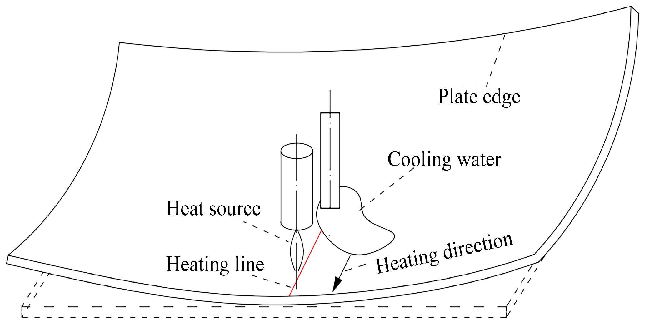
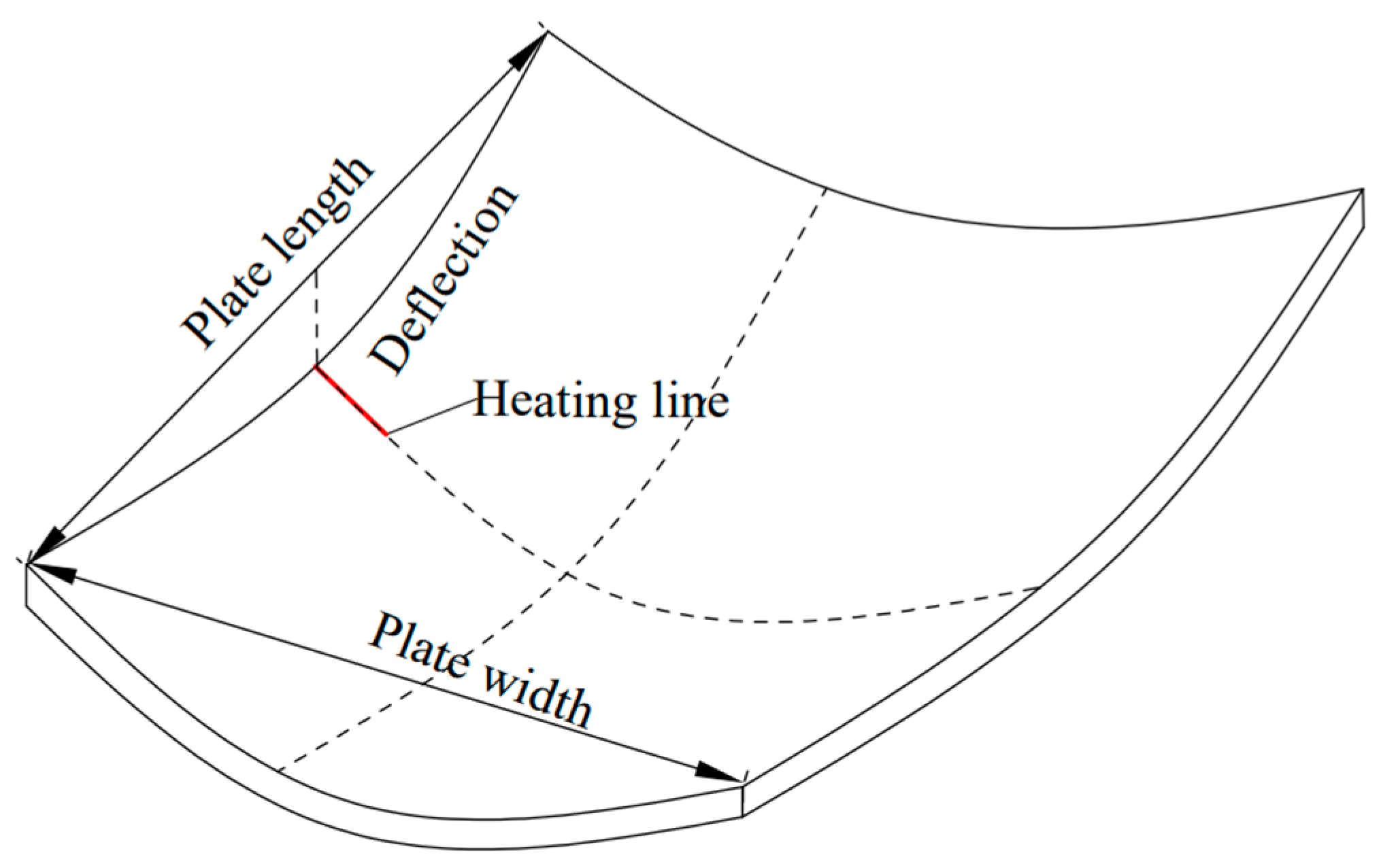
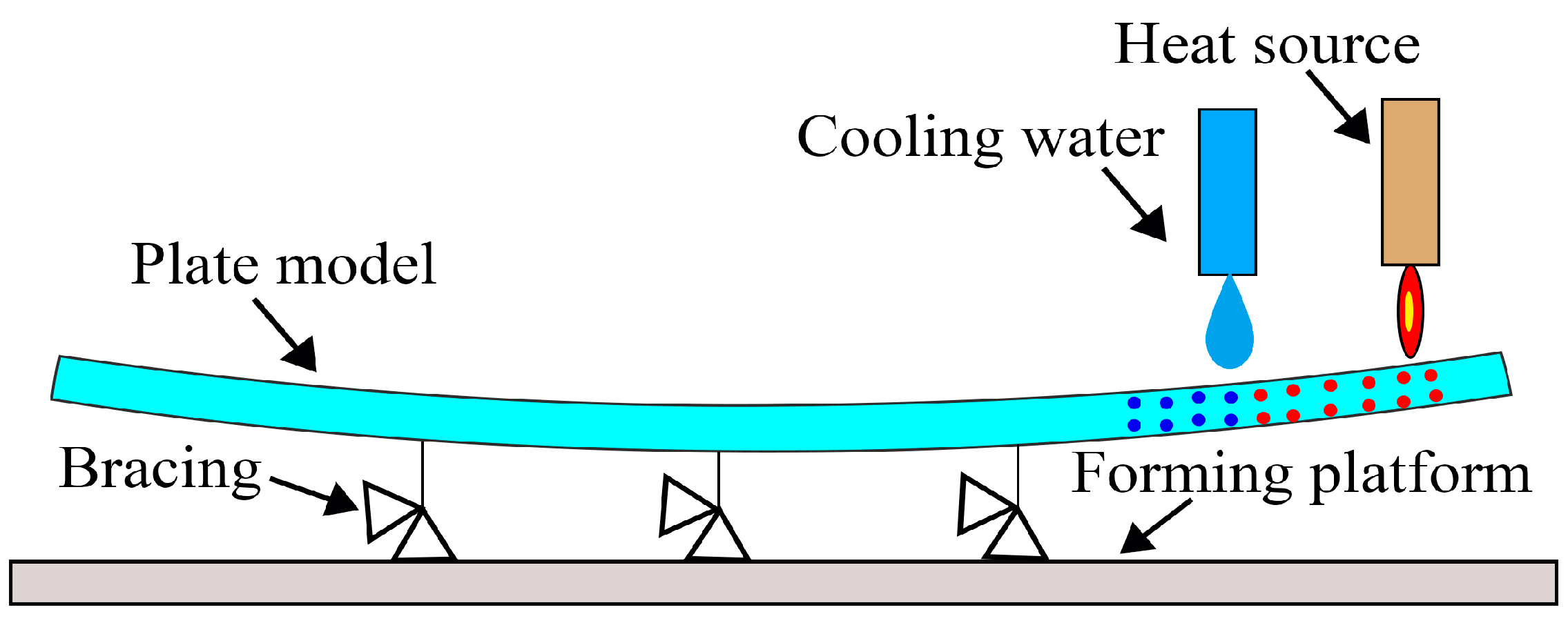
2.1. The Process of Line Heating

Line heating is a die-less forming technology. The heating method is local heating. The heat source is generally laser, electromagnetic, and flame. From an economic point of view, flame heating is the first choice for line heating. The line heating process is shown in Figure 1. Firstly, the heat source is preheated at the initial position of the heating line. After preheating, the heat source moves to the end of the heating line at a fixed speed. After the water cooling, the plate surface temperature is cooled to room temperature, and the line heating operation is completed.

As shown in Figure 2, the deformation changes in the process of heating and cooling. In the moving area of the heat source, the plate expands by heating. After stopping heating, the cooling water acts on the heating area. The temperature of the heating area decreases rapidly and shrinks until the temperature of the heating area tends to room temperature. The plate produces irreversible plastic deformation.

2.2. Numerical Simulation Theory of Titanium Alloy Line Heating

2.2.1. Heat Source Model

Combined with the actual processing, the heat source model generally selects the Gaussian heat source. The heat flux $q^{″}\left(r\right)$ at any point from the center of the heat source can be expressed by Formula (1):

$$q^{″}\left(r\right)=\frac{3Q{c}_3{H}_{6}A\eta }{\pi r_0^2}exp\left(-3{\left(\frac{r}{r_0}\right)}^2\right)$$

(1)

where $q^{″}\left(r\right)$ represents the heat flux density at any point on the surface of the titanium alloy plate model; $Q{c}_3{H}_6$ represents the flow rate of propylene fuel; $A$ represents the heat generated by the full combustion of propylene during the line heating of titanium alloy; $\eta$ denotes thermal efficiency; $r$ represents the distance between any point on the surface of the titanium alloy plate model and the center of the heat source; $r_0$ represents the effective radius of the heat source for the titanium alloy plate surface heating.

2.2.2. Thermal–Elastic–Plastic Theory of Titanium Alloy Line Heating

For titanium alloy materials, the relationship between stress and strain is linear in the elastic range of material deformation. When the deformation of the material exceeds the elastic range, the deformation of the material is irreversible. The relationship between stress and strain is nonlinear.

When the titanium alloy sheet is in the plastic or elastic state, the relationship between the stress and strain of the titanium alloy sheet is shown in Formula (2):

$$\left\{\mathrm{d}\sigma \right\}=\left[D\right]\left\{\mathrm{d}\epsilon \right\}-\left[C\right]\left\{\mathrm{d}T\right\}$$

(2)

where C is a vector, which is related to the surface temperature of the titanium alloy plate.

When the titanium alloy plate is in the state of elastic deformation, the elastic matrix $\left[D\right]$ can be obtained by Formula (3) and the elastic matrix $\left\{C\right\}$ can be obtained by Formula (4):

$$\left[D\right]={\left[D\right]}_e$$

(3)

$$\left\{C\right\}={\left\{C\right\}}_e={\left[D\right]}_e\left(\left\{\alpha \right\}+\frac{\mathit{\partial }{\left[D\right]}_e^{-1}}{\mathit{\partial }T}\sigma \right)$$

(4)

where $D_e$ represents the elastic matrix of the titanium alloy plate in the elastic state; $\mathsf{\alpha }$ represents the linear expansion coefficient of the titanium alloy plate.

When the titanium alloy plate is in the plastic deformation state, the plastic strain increment formula is shown in Formula (5).

$${\left\{{\mathrm{d}}_{\mathsf{\epsilon }}\right\}}_p=\lambda \left\{\frac{\mathit{\partial }f}{\mathit{\partial }\sigma }\right\}$$

(5)

where $f$ represents the yield function of the titanium alloy plate, $f\left(\sigma \right)=f_0\left({\epsilon }_p,T\right)$; $f_0$ represents the yield stress, which is related to the plastic strain and temperature of the titanium alloy plate.

In the process of the heat source movement, the material parameters of the titanium alloy change. The thermal–elastic–plastic problem of the titanium alloy plate in the line-heating process needs to be researched by incremental theory. The incremental theory establishes a constitutive equation based on the increment between stress and strain. The total stress and total strain generated during the line heating process of titanium alloy are obtained by the cumulative method.

The titanium alloy plate model is divided into several blocks with the same geometric size. Each block is an element. The equilibrium equation of any element of titanium alloy plate is shown in Formula (6):

$${\left\{\mathrm{d}F\right\}}^e+{\left\{\mathrm{d}R\right\}}^e={\left[\mathrm{K}\right]}^e{\left\{d\delta \right\}}^e$$

(6)

where ${\left\{\mathrm{d}F\right\}}^e$ represents the node force increment generated by any element of the titanium alloy plate; in the process of titanium alloy line heating forming, the heat source has an effect on the plate temperature. ${\left\{\mathrm{d}R\right\}}^e$ represents the equivalent increment of any element caused by the change in temperature gradient, which can be calculated through Formula (7). ${\left[K\right]}^e$ represents the stiffness matrix of any element of the titanium alloy plate model which can be calculated through Formula (8).

$${\left\{\mathrm{d}R\right\}}^e=\int {\left[B\right]}^T\left\{C\right\}\mathrm{d}T\mathrm{d}V$$

(7)

$${\left[K\right]}^e=\int {\left[B\right]}^T\left[D\right]\left[B\right]\mathrm{d}V$$

(8)

where $\left[B\right]$ denotes a matrix that relates the displacement vector and strain generated by any element node of the titanium alloy.

When the element of titanium alloy plate is in an elastic state, $\left[D\right]$ and $\left\{C\right\}$ are replaced by ${\left[D\right]}_e$ and ${\left\{C\right\}}_e$, respectively. The equilibrium equation of the whole plate is shown in Formula (9).

$$\left[K\right]\left\{\mathrm{d}\delta \right\}=\left\{\mathrm{d}F\right\}$$

(9)

where $\left[K\right]$ represents the stiffness matrix of the whole titanium alloy sheet, $\left[K\right]=\sum {\left[K\right]}^e$; $\left\{\mathrm{d}F\right\}$ represents the total load vector acting on titanium alloy sheet, $\left\{\mathrm{d}F\right\}=\sum \left(\right\{\mathrm{d}F{\}}^e+\left\{\mathrm{d}R{\}}^e\right)$.

In the process of titanium alloy line heating, it is generally not affected by external force. There is self-equilibrium of the nodal force around any element of titanium alloy plate. $\sum \{dF{\}}^e=0$, thus $\left\{dF\right\}=\sum \{dR{\}}^e$.

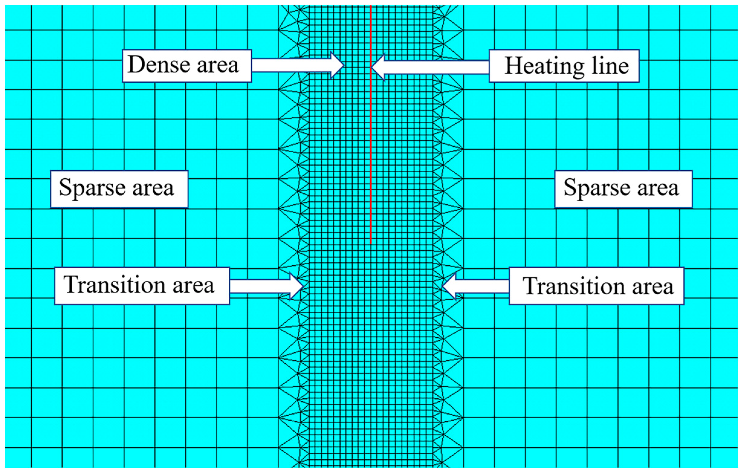
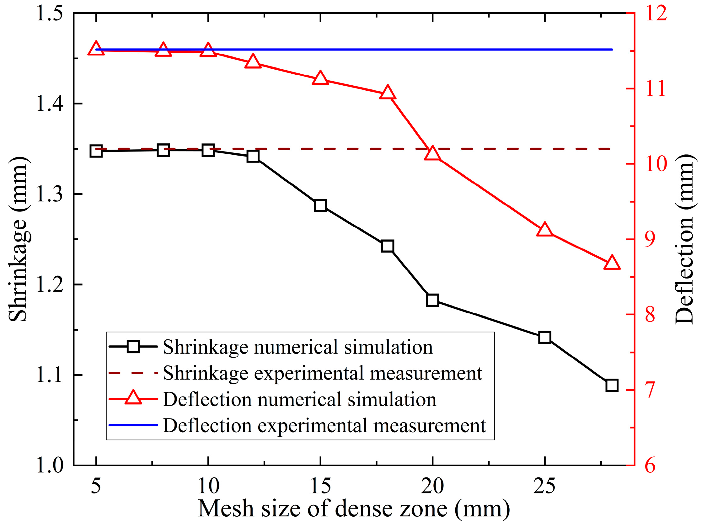
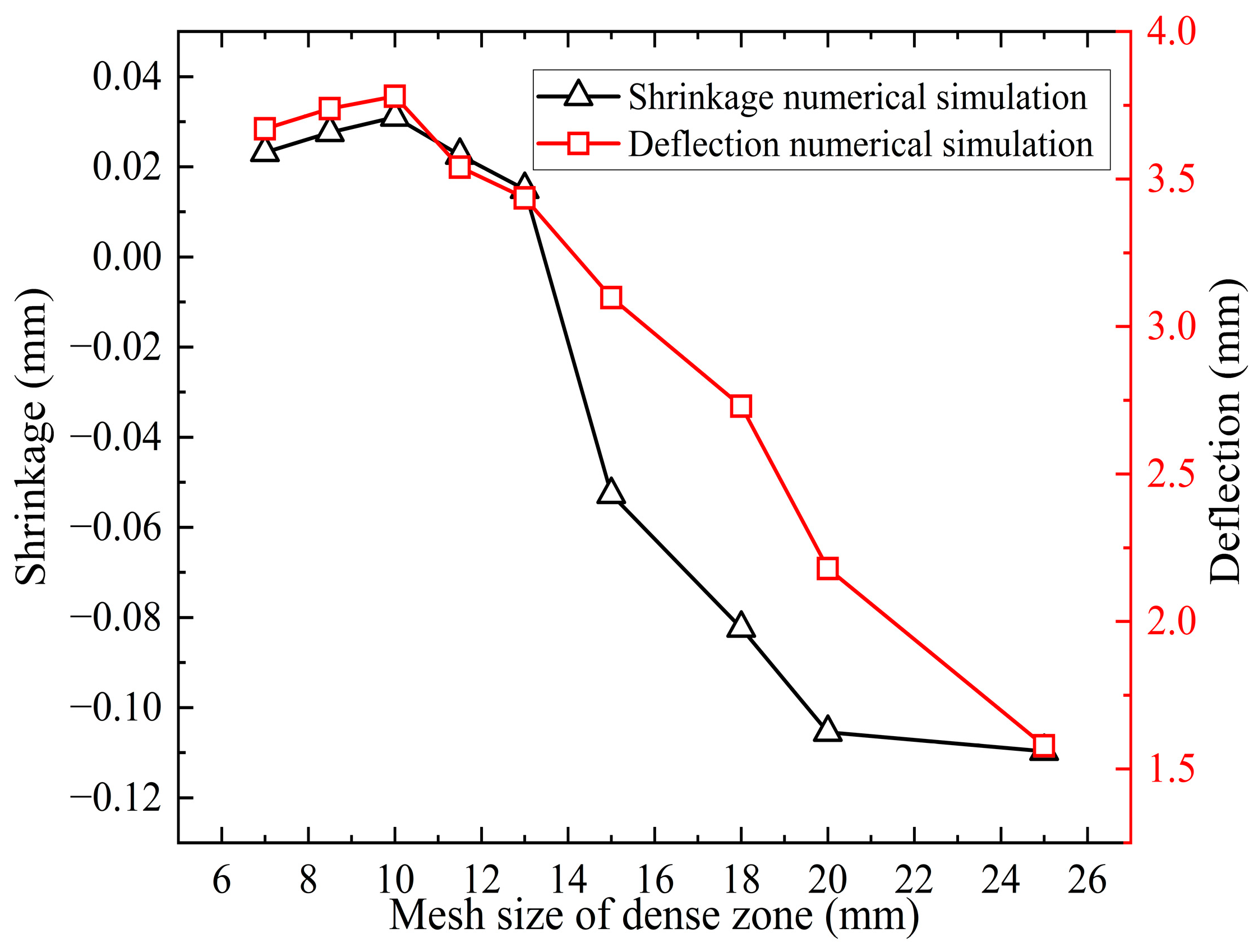
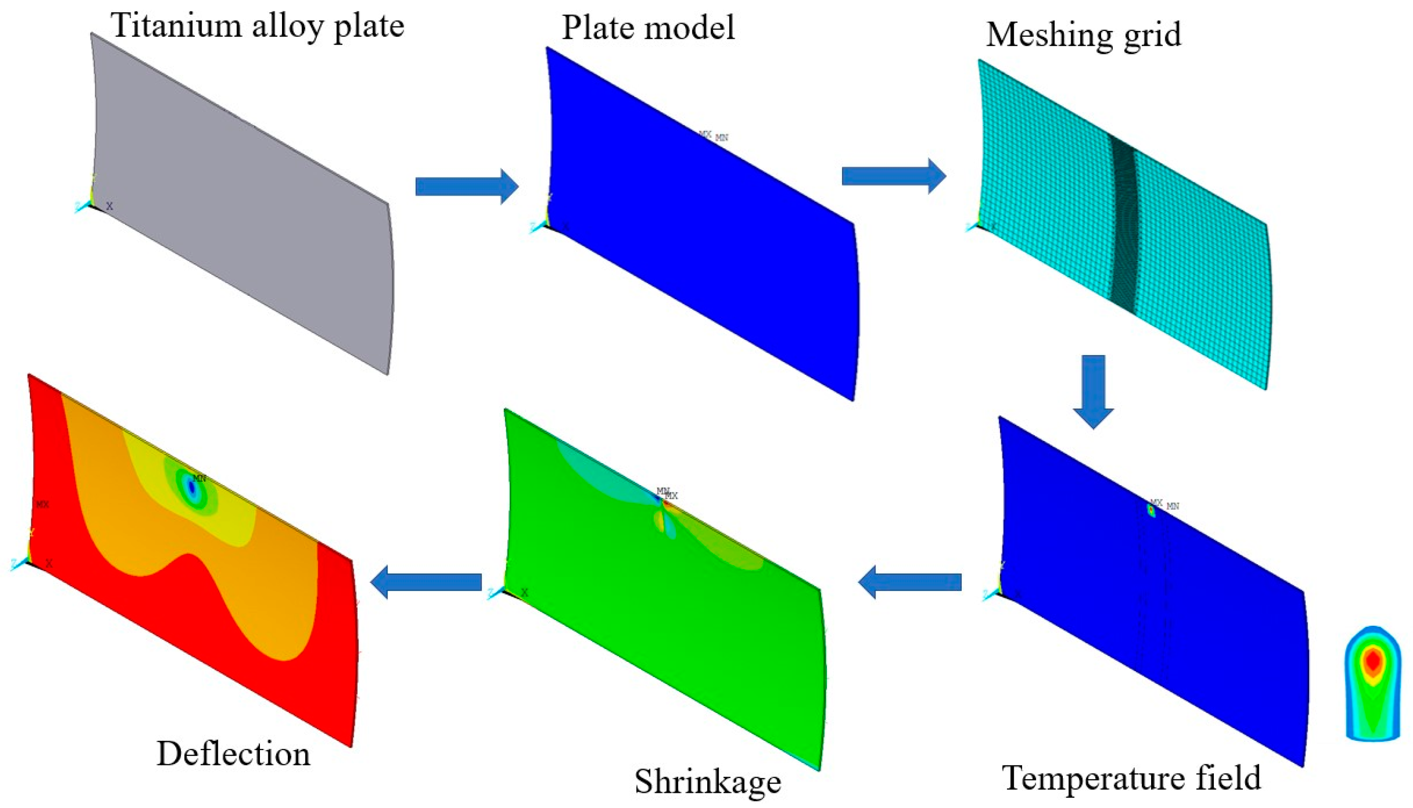
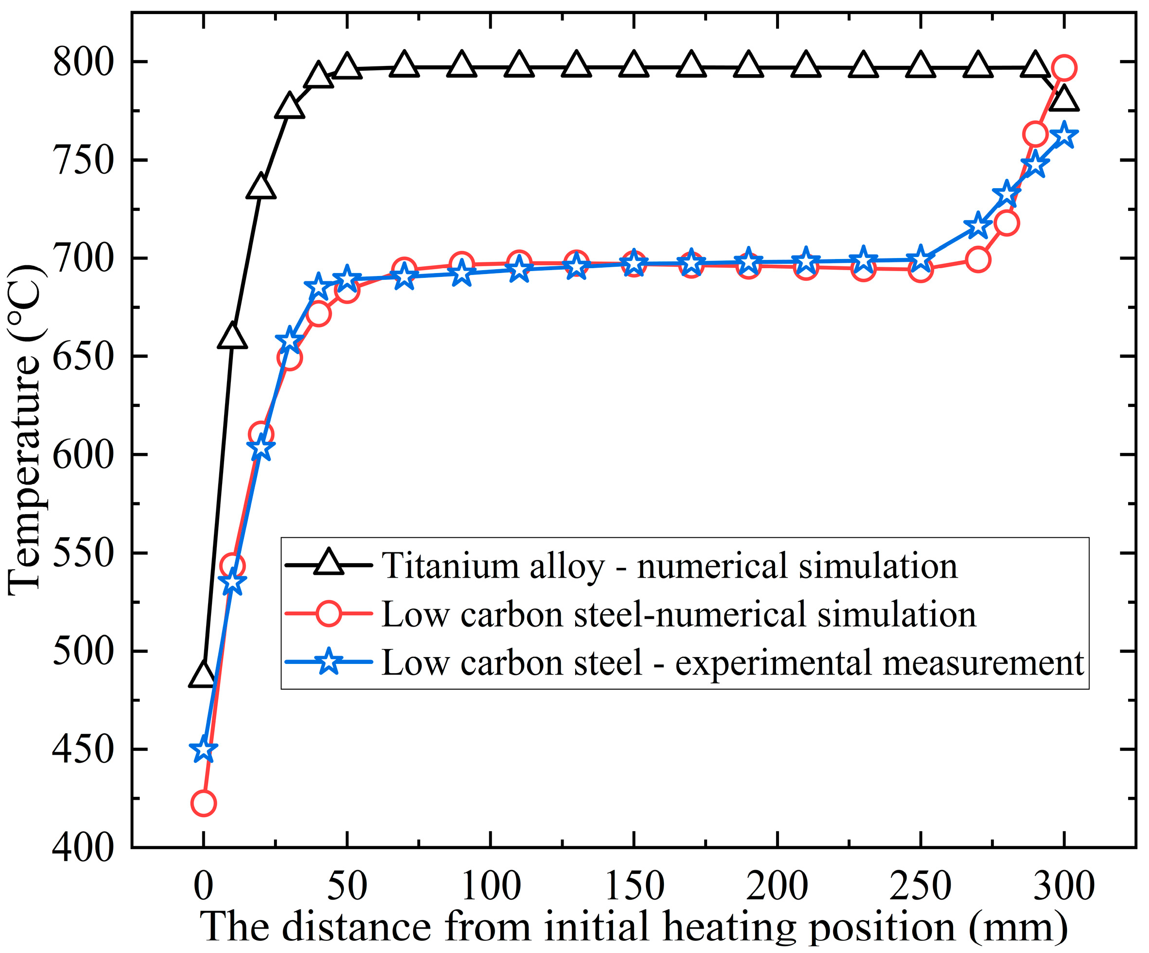
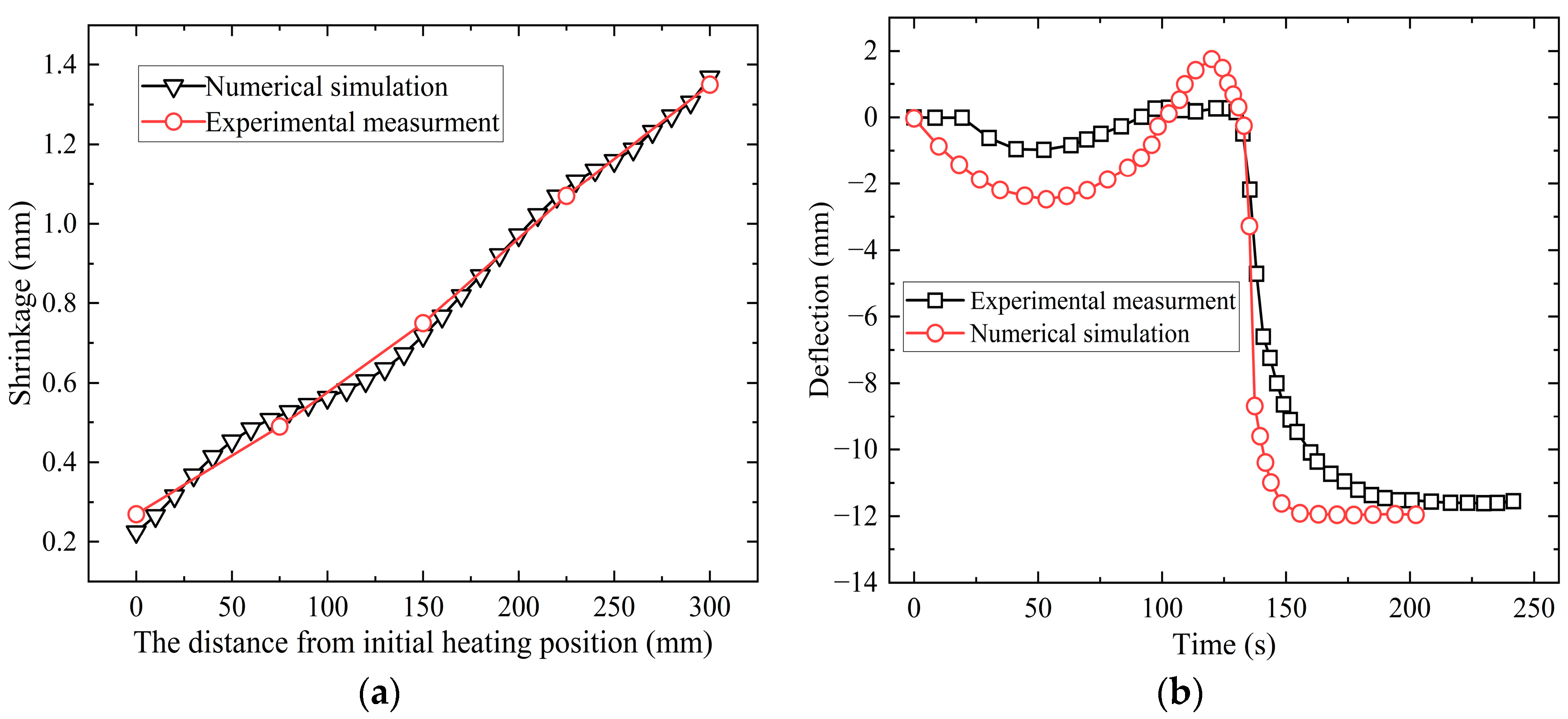
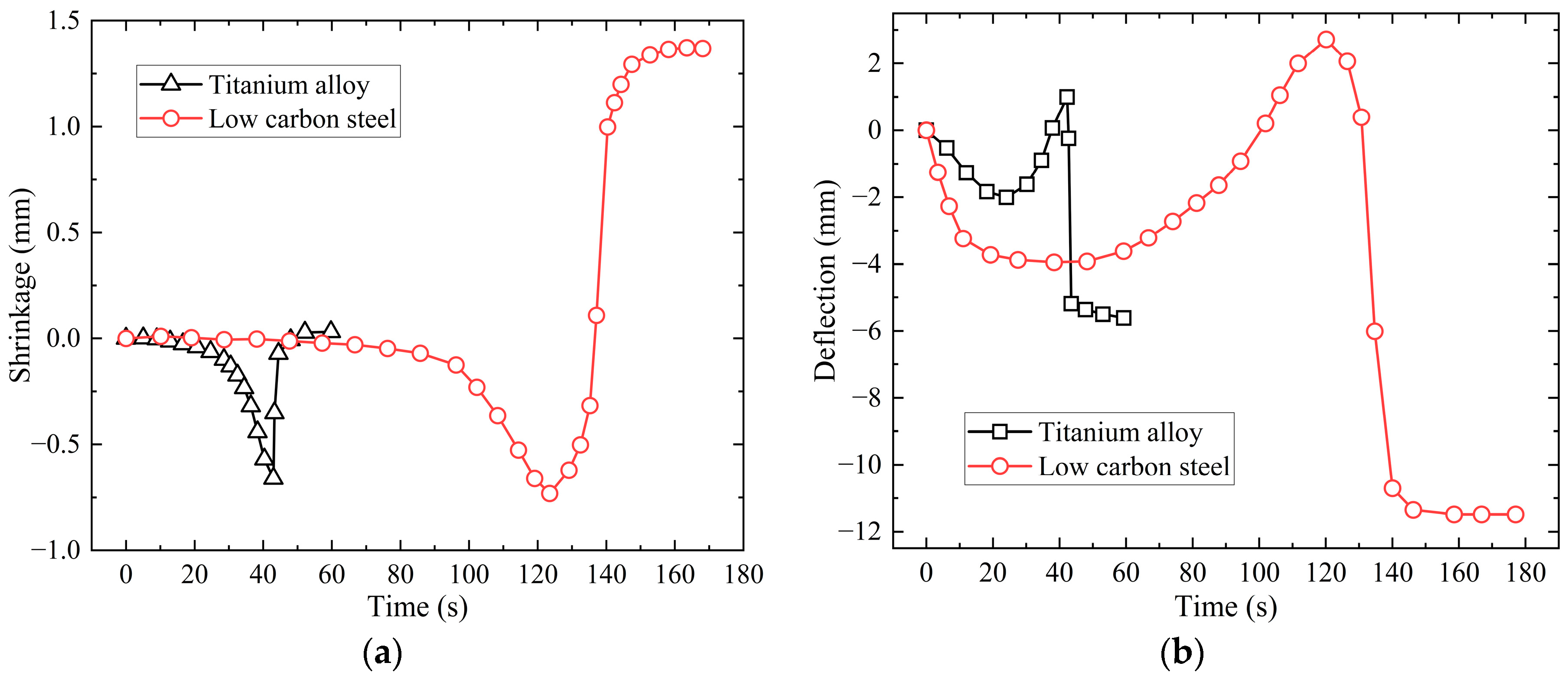
2.3. Feasibility Verification of Numerical Calculation of Titanium Alloy Line Heating

Based on the ANSYS 16.0 software platform, the model is parameterized by the APDL. The sketch map of line heating forming is shown in Figure 3. The geometric parameters of the plate are as follows: The plate length is 3 m. The plate width is 1.5 m. The plate thickness is 14 mm. The curvature radius of the plate is 5 m. Forming parameters are as follows: The heating line length is 0.3 m. The preheating time and heating time are set according to the plate type and the processing target value. The heat source used is a Gaussian heat source. The cooling method is tracking water cooling. The heat source and the tracking water cooling are moving along the heating line at the same speed. A fixed distance of 0.15 m is maintained between the heat source and the tracking water cooling. The ambient temperature is set to 20 °C.

In the numerical calculation process of titanium alloy line heating, the heating line position and the meshing are shown in Figure 4. The heating line is perpendicular to the edge of the upper plate. The endpoint of the heating line is located at the midpoint of the upper plate edge. The area where the heat source moves, the temperature gradient changes greatly, and is divided into the dense area. For the area far away from the heat source, the temperature gradient changes little and is divided into sparse areas. The transition region is located between the sparse region and the encrypted region. Meshing each region with different sizes can reduce the numerical calculation time and avoid the influence of mesh size on the results.

In order to obtain the influence of different mesh sizes on the calculation results, several mesh size schemes in

Table 1. Different mesh size schemes.

Dense Zone Grid (mm)	Transition Zone Grid (mm)	Sparse Zone Grid (mm)
7	14	35
8.5	17	42.5
10	20	50
11.5	23	57.5
13	26	65
15	30	75
18	36	90
20	40	100
25	50	125

are designed.

Under different mesh sizes, the temperature of the plate length position on the heating line side of titanium alloy and low-carbon steel is shown in Figure 5. The mesh size of low-carbon steel and titanium alloy in the dense area is less than 10 mm, and the temperature of the coincidence point between the upper plate margin and the heating line obtained by each mesh scheme is close. The error of the temperature result is less than 1% through each scheme.

The calculation of the deformation field includes shrinkage and deflection, the measurement method is referred to in reference [25]. The shrinkage of low-carbon steel and titanium alloy under different grid sizes is shown in Figure 6 and Figure 7, respectively. When the mesh size of the dense zone is less than 10 mm, the shrinkage and deflection of the numerical simulation is close to that of the experiment. The error between adjacent mesh schemes is less than 5%. When the mesh size of titanium alloy in the dense area is less than 10 mm, the difference between the shrinkage and deflection obtained by each scheme is small. When the mesh size of the dense area is greater than 10 mm, with the increase in the mesh size, the shrinkage and deflection obtained gradually decrease. The independence of numerical model grids is verified. The mesh size of the dense area is set to 10 mm, the mesh size of the transition area is set to 20 mm, and the mesh size of the sparse area is set to 50 mm.

In the actual processing process, the pillow is cushioned at the end of the board width direction to promote the forming. Combined with the actual processing experience, the constraints set are shown in Figure 8. The LINK180 unidirectional tensile spring support is set at one-fourth, one-half, and three-fourth positions in the width direction of the two sides of the plate. The numerical calculation process of titanium alloy line heating is shown in Figure 9. The numerical simulation of line heating for plate forming includes the calculation of the temperature field and deformation field. The heat generated due to the plate deformation is little, which can be ignored. Therefore, the numerical simulation of the steel plate line heating forming adopts the sequential coupling method. Firstly, the temperature field in the process of heat source moving is solved. To solve the temperature field, it is necessary to define the time step. The numerical calculation model can converge when the time step is reasonable. If the time step is too large, the numerical calculation model may not converge. If the time step is too small, it will increase the calculation time. Secondly, the deformation field is solved based on the temperature field. In this process, the solution results of the temperature field are applied as a load to the deformation field calculation.

The numerical calculation model material type is set to TA5 titanium alloy. The thermal conductivity, specific heat capacity, Poisson’s ratio, and linear expansion coefficient of TA5 titanium alloy at different temperatures are shown in

Table 2. Material parameters of TA5 titanium alloy at different temperatures.

Temperature (°C)	Coefficient of Thermal Conductivity (W/m °C)	Heat Capacity (J/kg °C)	Poisson’s Ratio	Coefficient of Linear Expansion (10−6/°C)
20	7.71	513	0.34	9.28
100	8.83	523	0.43	9.53
200	10.3	537	0.34	9.87
300	11.9	554	0.35	10.08
400	13.6	572	0.37	10.09
500	15.4	594	0.38	10.28
600	17.3	617	0.39	10.56
700	19.3	643	0.40	11.66
800	21.4	671	0.42	13.04
900	23.7	701	0.43	14.42
1000	26	734	0.44	15.8

[26]. At room temperature, the linear expansion coefficient is small, and it is not easy to deform. The thermal conductivity, specific heat capacity, Poisson’s ratio, and linear expansion coefficient of titanium alloy are positively correlated with the temperature. The chemical composition of TA5 titanium alloy is shown in

Table 3. Chemical composition of TA5 titanium alloy.

Chemical composition	Al	B	Fe	Si	C	N	H	O
Mass fraction (%)	4.36	0.0039	0.0390	0.01	0.012	0.008	0.01	0.13

.

The numerical calculation models of titanium alloy and low-carbon steel have the same parameters and processing methods except for preheating time, heating time, and material parameters. The preheating time of titanium alloy is 1 s and the heating time is 40 s. The preheating time of low-carbon steel is 5 s and the heating time is 130 s. The maximum temperature variation on the heating line of titanium alloy and low-carbon steel is shown in Figure 10. The numerical simulation and experimental measurement of the plate edge of the low-carbon steel heating line side are 788.13 °C and 762.32 °C, respectively [27]. The numerical simulation results of the maximum temperature of each point on the low-carbon steel heating line are in agreement with the experimental measurement results. The maximum temperature variation law of titanium alloy and low-carbon steel on the heating line is similar. Through numerical simulation, the maximum temperature of the plate edge of the titanium alloy heating line side is 779.69 °C. The thermal conductivity of low-carbon steel is negatively correlated with the temperature. The thermal conductivity of titanium alloy is positively correlated with the temperature. Therefore, compared with the maximum temperature of each point in the range of 50 mm to 270 mm on the titanium alloy heating line, the maximum temperature decreased. The feasibility of the numerical calculation model of titanium alloy to calculate the temperature field has been verified.

The experimental measurement and numerical simulation of the deformation field of low-carbon steel are shown in Figure 11. The shrinkage of the plate edge of the titanium alloy heating line side is 1.39 mm and 1.35 mm, respectively. The numerical simulation and experimental measurement are consistent. The final deflection is 11.60 mm, and the final deflection of the numerical simulation is 11.96 mm. The numerical simulation results are reliable. The variation law of the deformation field is shown in Figure 12. The deflection and shrinkage of the two materials at the plate edge of the titanium alloy heating line side are similar. Through numerical simulation, the shrinkage and deflection of the plate edge of the titanium alloy heating line side are 0.031 mm and 5.47 mm, respectively. The linear expansion coefficient of titanium alloy is smaller than that of low-carbon steel, and the deformation is smaller than that of low-carbon steel. The feasibility of the numerical calculation model of titanium alloy is verified, which can be applied to the calculation of the deformation field.

Based on the model of a single heating line, the model of overlapping heating of titanium alloy is established. After heating three times at the same position, the temperature field and deformation field changes at the plate edge of the titanium alloy heating line side are shown in Figure 13. The shrinkage and deflection of the edge position of the titanium alloy plate are 1.01 mm and 20.34 mm, respectively. In the three-times heating process, the temperature, shrinkage, and deflection of the plate edge of the titanium alloy heating line side are consistent with the law of the single heating process. In summary, the feasibility of the numerical calculation model of overlapping the heating of titanium alloy has been verified, which can be applied to the calculation of the temperature field and deformation field.

3. Research of the Deformation Prediction Model of Titanium Alloy Overlap Heating

There are many factors involved in the research of overlapping heating of titanium alloy line heating. If the data between the influencing factors and the deformation are obtained through experiments, the experimental cost is high. If the numerical simulation method is used, the calculation amount is large and the time cost is high. Therefore, an intelligent algorithm is used to establish a prediction model that can achieve rapid prediction and meet the accuracy requirements.

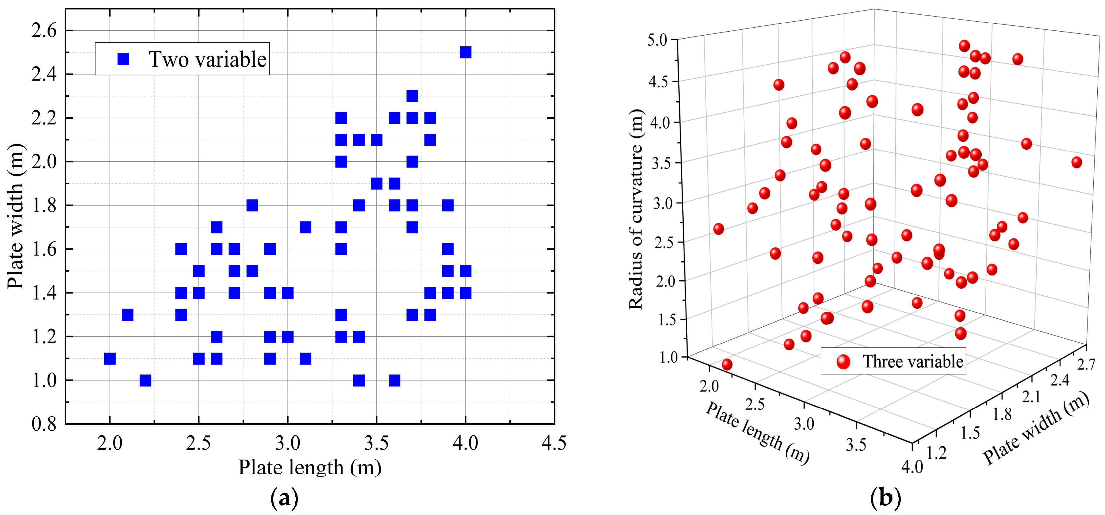
3.1. Sample Sampling and Data Processing

To research the effect of line heating of the titanium alloy plate under different geometric parameters and forming parameters, and to ensure the randomness of the selected test scheme, Latin hypercube sampling is selected in the sampling method. When the plate length and plate width are variables, according to the requirements of titanium alloy line heating, the length–width ratio is not less than 1.5. After Latin hypercube sampling, the sample distribution is shown in Figure 14a. Due to the limitation of conditions, the data of the upper left position in Figure 14a do not meet the sampling conditions. When the plate length, plate width, and curvature radius are taken as variables, on the basis of sampling with plate width and plate length as variables, the restriction condition is added, and the radius of curvature is required to be greater than 1. After Latin hypercube sampling, the sample distribution is shown in Figure 14b.

The sample distribution satisfies the randomness of Latin hypercube sampling, so the Latin hypercube sampling is applied. By adding constraints, the sampling scheme meets the requirements of titanium alloy line heating. Five variables are selected in the experimental design, including plate length, plate width, curvature radius, plate thickness, and heating line length. The single heating time is determined by plate thickness and heating line length. The sampling interval is selected as follows: The plate length ranges from 2 m to 4 m. The plate width ranges from 1 m to 2.5 m. The curvature radius ranges from 1 m to 5 m. The plate thickness ranges from 8 mm to 28 mm. The heating line length ranges from 0.2 m to 0.4 m. On the basis of the sampling with the previous three factors as variables, the heating line length is required to be less than a quarter of the plate width.

Through Latin hypercube sampling, 73 groups of numerical calculation schemes for titanium alloy forming are obtained. According to the numerical calculation model of titanium alloy forming, the numerical calculation results of the forming schemes are obtained, as shown in

Table 4. The 73 groups of numerical calculation results for titanium alloy forming.

No.	Plate Length (m)	Plate Width (m)	Curvature Radius (m)	Plate Thickness (mm)	Heating Line Length (mm)	Heating Time (s)	Shrinkage (mm)	Deflection (mm)
1	2.6	1.2	1.4	8	0.2	22	0.876	8.89
2	2.9	1.6	3.8	28	0.3	65	0.227	3.38
3	3.1	1.7	2.4	12	0.3	34	0.981	10.92
4	3.8	1.4	3.7	16	0.2	28	0.171	8.42
5	3.4	1.2	3.4	20	0.3	44	0.723	13.52
6	3	1.2	1.9	24	0.3	51	0.387	4.349
7	3.4	1.2	2.5	28	0.2	40	0.163	2.84
……	……	……	……	……	……	……	……	……
71	3.1	1.1	2	16	0.2	28	0.171	4.94
72	3.7	2.2	4.8	20	0.3	44	0.771	12.63
73	2.6	1.2	1.4	8	0.2	22	0.876	8.89

.

If the original data are not normalized, it is easy to cause problems such as saturation of neuron output in model training. Therefore, the data in Table 4 are normalized, and each row of data is normalized to an interval of 0 to 1. The input data are converted into a dimensionally consistent data matrix. Normalization formulas such as Formula (10):

$$Y=\left(Y_{max}-Y_{min}\right)\frac{X-X_{min}}{X_{max}-X_{min}}+Y_{max}$$

(10)

where $Y$ represents the normalized data matrix; $Y_{min}$ represents the minimum value of each row of the data matrix; $Y_{max}$ represents the maximum value of each row of the data matrix; $X$ represents the original data matrix; $X_{min}$ represents the minimum value of the original data matrix; $X_{max}$ represents the maximum value of the original data matrix.

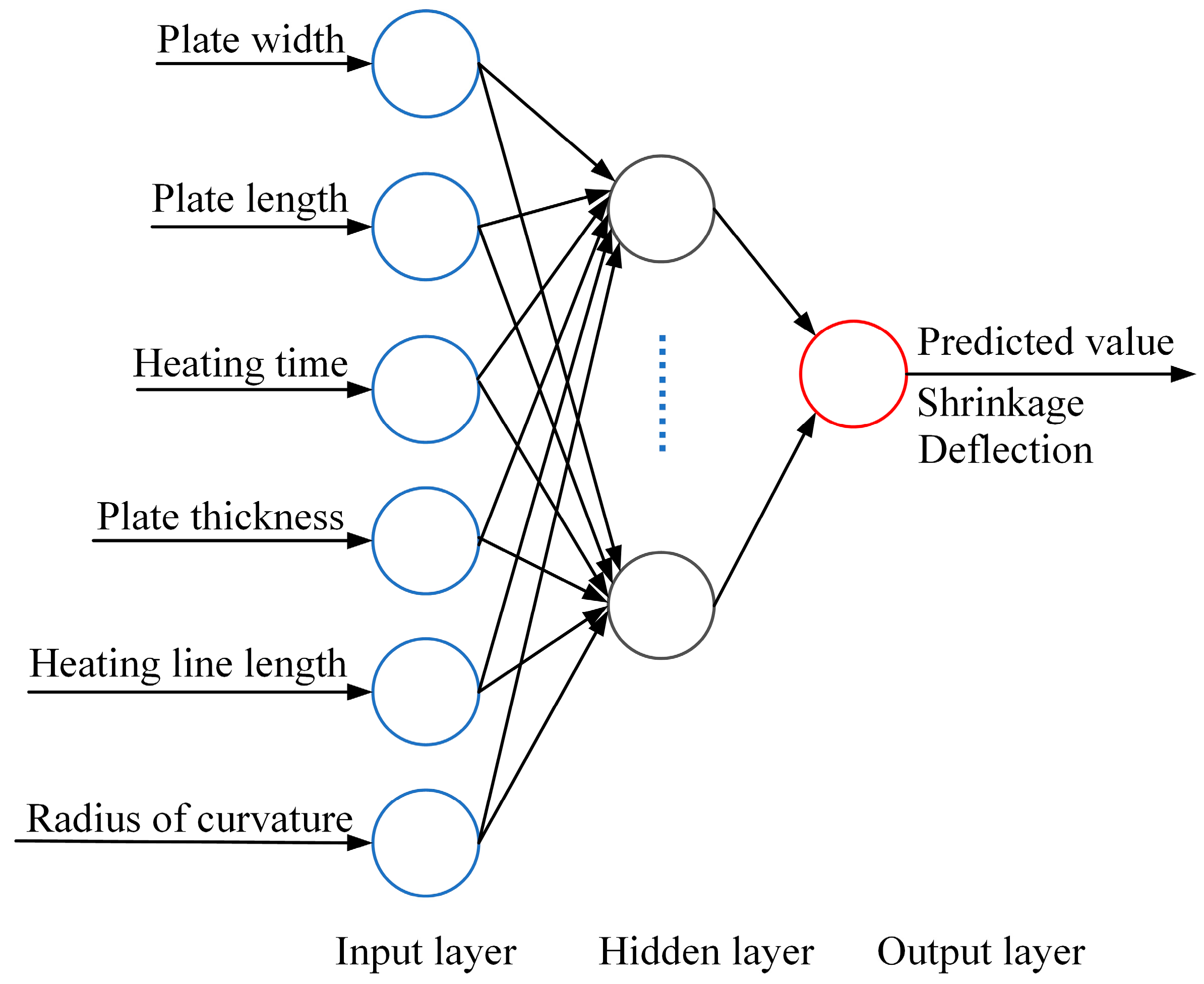
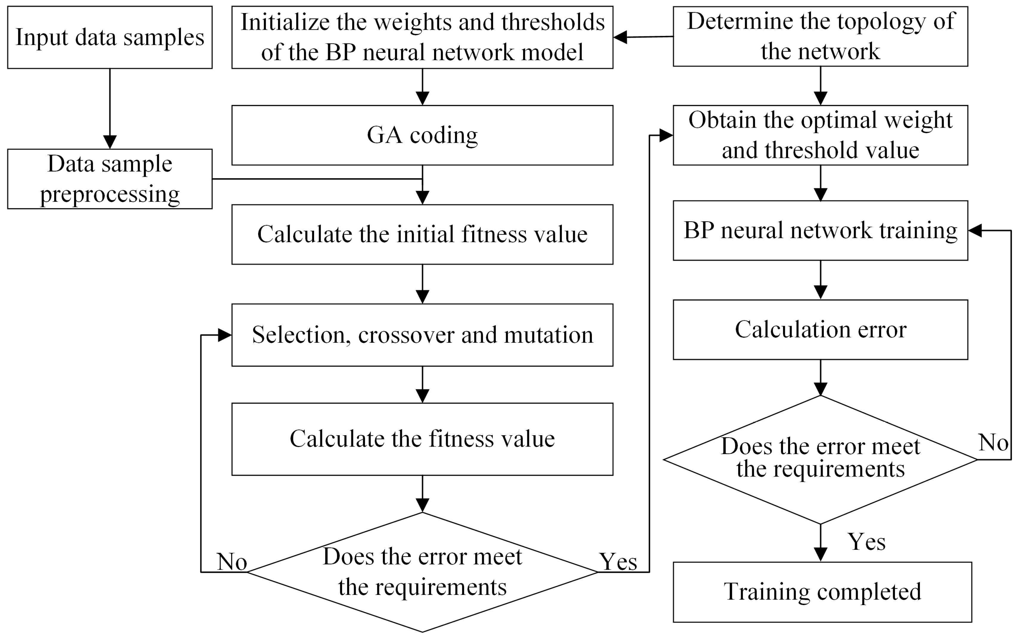
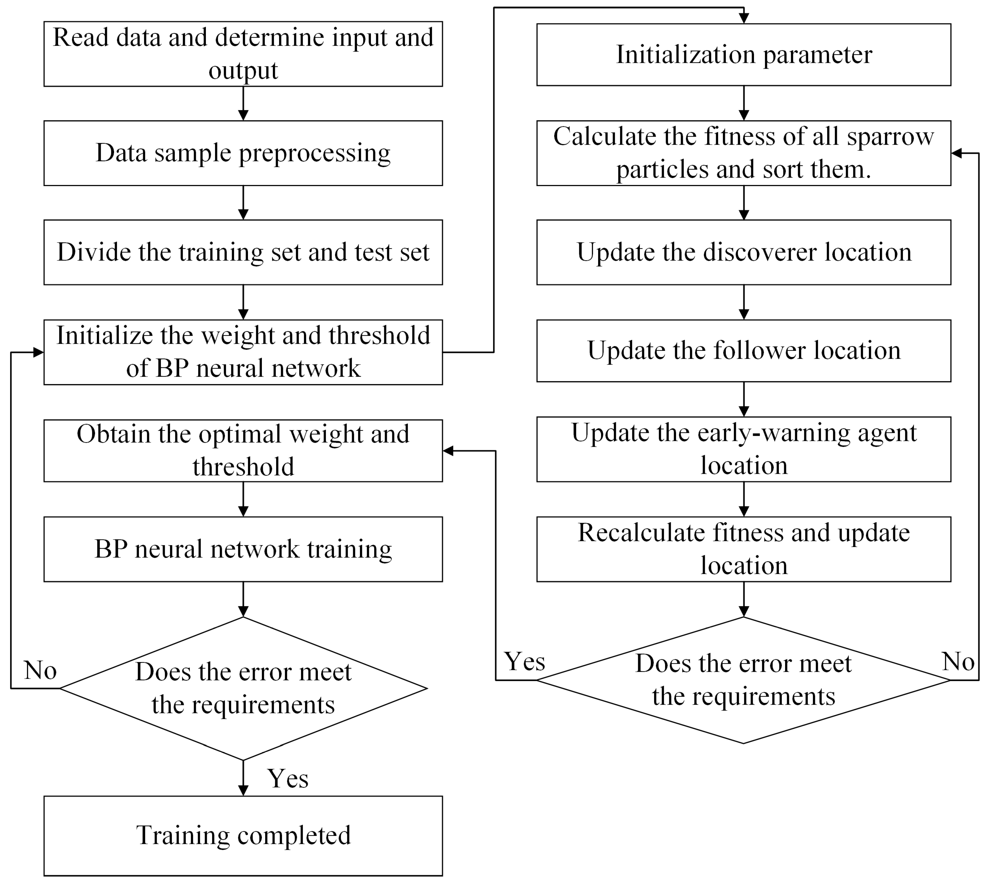
3.2. Prediction Model of Titanium Alloy Overlapping Heating Deformation Based on BP Neural Network Algorithm

The BP neural network can simulate human thinking, which is characterized by distributed storage and parallel collaborative processing of information. The BP neural network has good generalization ability, prediction ability, and control ability for samples that have not been trained. The BP neural network structure of titanium alloy-forming deformation prediction is shown in Figure 15. The BP neural network model is composed of input layer, hidden layer, and output layer. The input layer inputs the prediction sample parameters. The prediction sample parameters are refined by the hidden layer, and the prediction results are output from the output layer. The input parameters are six, including plate length, single heating time, heating line length, curvature radius, plate thickness, and plate width. The predicted targets are shrinkage and deflection. Due to the different difficulty of prediction, the two prediction targets are predicted, respectively, to improve the prediction accuracy. Therefore, the input layer contains six neurons, the output layer contains one neuron, and the number of hidden layers is set to one layer.

The propagation process of BP neural network is divided into signal forward propagation and error backpropagation.

Forward propagation calculation of BP neural network signal.

Determine the input sample and output sample.

$w_{gh}$ is set as the initial weight. Input $x_q=\left[x_{1q},x_{2q},\dots ,x_{nq}\right]$, the expected output $d_q=\left[d_{1q},d_{2q},\dots ,d_{mq}\right]$. When the node $g$ is input in the q group of samples, the output $y_{gq}$ can be calculated by Formula (11):

$$y_{gq}\left(t\right)=f\left(\sum _g{w}_{gh}\left(t\right)I_{hq}\right)$$

(11)

where $w_{gh}\left(t\right)$ represents the weight from the input layer to the hidden layer, which has undergone t adjustments. $I_{gq}$ represents that the input layer is the h th input of the neuron g in the sample input of the q th group.

Calculate the objective function $E_q$ and the total objective function $J\left(t\right)$ through Formulas (12) and (13).

$$E_q\left(t\right)=\frac{1}{2}\sum _k{{\left[d_{kq}-y_{kq}\left(t\right)\right]}^2=\frac{1}{2}}_{}\sum _k{e}_k^2\left(t\right)$$

(12)

$$J\left(t\right)=\sum _q{E}_q\left(t\right)$$

(13)

where $E_q$ represents the objective function; $y_q\left(t\right)$ represents the input sample q output after t times weight adjustment; k represents the kth neuron in the output layer; $J\left(t\right)$ represents the total objective function.

BP neural network error backpropagation calculation

$$\begin{gathered} w_{gh}\left(t+1\right)=w_{gh}\left(t\right)-\delta \frac{\mathit{\partial }J\left(t\right)}{\mathit{\partial }{w}_{gh}\left(t\right)}=w_{gh}\left(t\right)-\delta \sum _q\frac{\mathit{\partial }{E}_q\left(t\right)}{\mathit{\partial }{w}_{gh}\left(t\right)} \\ =w_{gh}\left(t\right)+\mathsf{\Delta }{w}_{gh}\left(t\right) \end{gathered}$$

(14)

where $w_{gh}\left(t+1\right)$ represents the weight from neuron h to neuron g after t + 1 times adjustments; δ is a constant.

Based on the BP neural network algorithm, the prediction model of titanium alloy overlapping heating deformation is established. There are 73 groups of normalized data samples. The samples are divided into training sets and prediction sets according to the ratio of 8:2. Under different numbers of hidden layer nodes, the mean square error of the training set is shown in Figure 16. When the prediction model is used to predict the shrinkage, the mean square error of the training set is the smallest when the number of hidden layer neurons is 5. When the prediction model is used to predict the deflection, the mean square error of the training set is the smallest when the hidden layer neurons number is 7. When the BP neural network model predicts the shrinkage of titanium alloy, the number of hidden layer neurons is set to 5. When predicting the deflection, the hidden layer neurons number is set to 7. The formula to calculate the mean square error (MSE) is shown in Formula (15).

$$\mathrm{M}\mathrm{S}\mathrm{E}=\frac{1}{n}\sum _{i=1}^n{\left(y_i-y_i^{\prime }\right)}^2$$

(15)

where $y_i$ represents the true value; $y_i^{\prime }$ represents the predicted value; $n$ represents the number of samples.

By setting the activation function of the BP neural network, non-linear factors are added to the neurons. The BP neural network model can approximate any nonlinear function. The training times and training rate affect the training time and prediction accuracy. The experimental parameters of the activation function, training times, and training rate are designed as follows: The activation function is set to ‘tansig’, ‘logsig’, and ‘purelin’. The training times are set to 8000, 10,000, 12,000, 14,000, and 16,000. The learning rate is set to 0.1, 0.01, and 0.001. The parameter design of the prediction model is shown in

Table 5. BP neural network training parameters optimization scheme.

No.	Activation Function	Training Times	Training Rate
1	‘tansig’	8000	0.1
2	‘tansig’	8000	0.01
3	‘tansig’	8000	0.001
4	‘tansig’	10,000	0.1
5	‘tansig’	10,000	0.01
⋯	⋯	⋯	⋯
43	‘purelin’	16,000	0.1
44	‘purelin’	16,000	0.01
45	‘purelin’	16,000	0.001

.

The prediction accuracy was evaluated through mean absolute percentage error (MAPE) and goodness of fit (R²). The closer the MAPE is to 0, the smaller the absolute value of the relative error between the predicted value and the true value. The closer the R² is to 1, the higher the prediction accuracy. MAPE and R² are calculated by Formulas (16) and (17), respectively.

$$\mathrm{M}\mathrm{A}\mathrm{P}\mathrm{E}=\frac{1}{n}\sum _{i=1}^n{\left|\frac{\left(y_i-y_i^{\prime }\right)}{y_i}\right|}^{}\times 100\%$$

(16)

$$R^2=\sum _{i=1}^n{{\left(y_i^{\prime }-{\overline{y}}_i\right)}^2}^{}/\sum _{i=1}^n{{\left(y_i-{\overline{y}}_i\right)}^2}^{}$$

(17)

where ${\overline{y}}_i$ represents the mean value of the numerical value.

In Table 5, R² and MAPE under different schemes are shown in Figure 17. The R² and MAPE of group 11 were 0.986 and 7.45%, respectively, which are better than those of the other 44 groups.

The BP neural network is sensitive to the initial network weight. When the network is initialized with different weights, it tends to converge to different local minima. In order to improve the shortcomings of traditional BP neural network prediction, the optimal initial weights and thresholds are searched by GA and SSA algorithms to improve the prediction accuracy.

Compared with the BP neural network, the GA algorithm has better global optimization ability and is not limited by connection function. Optimizing the BP neural network by GA algorithm can improve the defect that the BP neural network is easy to fall into the local minimum. The training process of the GA-BP model is shown in Figure 18. The GA algorithm can automatically obtain the search direction of the search space and adjust the direction. The GA algorithm establishes a cyclic iterative optimization process by simulating the natural selection, hybridization, and mutation evolution of genes in natural genetics. The adaptability of the optimal individual is further improved and the final global optimal solution is obtained. The initial population size of the GA-BP model is set to 60. The maximum number of evolutions is set to 80. The crossover probability is set to 0.8. The mutation probability is set to 0.2. The upper limit of the adaptive variable is set to 3, and the lower limit is set to −3. Through the GA algorithm, the BP neural network can be searched for relatively excellent initial weights and thresholds, and the number of iterations of the BP neural network can be reduced.

The advantages of the SSA algorithm are as follows: The parallelism is excellent [24]. The ability of global search is strong. The speed of convergence is fast. The SSA algorithm divides the sparrow population by simulating sparrow predation and anti-predation. Sparrows are classified into three types: discoverers, followers, and early-warning agents. The finder is responsible for providing foraging directions and areas. The followers follow the finder foraging. The early-warning agent is responsible for monitoring the foraging area. In the process of foraging, the positions of the three are constantly updated to complete resource acquisition. The training flow chart of the SSA-BP model is shown in Figure 19. The early-warning agent appears randomly in the population. Through the position of the three, we find out the global optimal position. The global optimal position is found by the positional relationship of the three. The SSA algorithm can find the optimal initial weights and thresholds for the BP neural network so that the neural network error is near the global minimum at the beginning of training. The population size of the SSA-BP model is set to 20. The upper limit of iteration times is set to 30. The upper limit of the weight and threshold is set to 5, and the lower limit is set to −5.

The location of the discoverer can be calculated by Formula (18).

$$x_{ij}^{t-1}=\left\{\begin{array}{ll}{x}_{ij}^t.exp\left(\frac{-i}{\alpha .{iter}_{max}}\right),& R_2<ST\\ x_{ij}^t+Q.L,& {R_2\ge ST}^{}\end{array}\right.$$

(18)

The position of the follower can be calculated by Formula (19).

$$x_{ij}^{t+1}=\left\{\begin{array}{ll}Q.exp\left(\frac{x_{worst}^t-x_{ij}^t}{\alpha .{iter}_{max}}\right),& i<a/2\\ x_p^{t+1}+\left|x_{ij}^t-x_p^{t+1}\right|.{A^{+}}^{}.L,& {otherwise}^{}\end{array}\right.$$

(19)

where a represents the number of sparrows; $x_{ij}^{}$ represents the location of sparrows in the population; $i$ represents the number of ongoing iterations of the algorithm; ${iter}_{max}$ represents the number of iterations set by the algorithm; $\alpha$ and Q are randomly generated constants; $0<\mathsf{\alpha }<1$; $L$ represents a matrix with a row number of 1 and a column number of d, in which all elements are 1; $R_2$ and $ST$ are the safety factor and warning coefficient, respectively; $x_p^{}$ and $x_{worst}^t$ represent the best area and the worst area searched by the sparrow particle as the discoverer, respectively; $A^{}$ represents a matrix with a row number of 1 and a column number of d, in which all elements are 1 or −1; $A^{+}=A^T{\left(A{A}^T\right)}^{-1}$.

The position of the early-warning agent can be calculated by Formula (20).

$$x_{ij}^{t+1}=\left\{\begin{array}{cc}{x}_{best}^t+\beta \left|x_{ij}^t-x_{best}^t\right|,& f_i>f_g\\ x_{ij}^t+k.\left(\frac{\left|x_{ij}^t-x_{best}^t\right|}{f_i-f_w+\epsilon }\right),& f_i=f_g\end{array}\right.$$

(20)

where $x_{best}^t$ represents the optimal region for all sparrow particles found; $\beta$ and $k$ are random numbers; $\beta$ obeys standard normal distribution; $-1<k<1$; $f_i$ represents the fitness value of sparrow particles; $f_i$ and $f_g$ represent the fitness values of the best and worst regions found by all sparrow particles, respectively; the minimum parameter $\epsilon$ is introduced to avoid zero denominator.

4. Results and Analysis of Overlapping Heating Deformation Prediction Model of Titanium Alloy

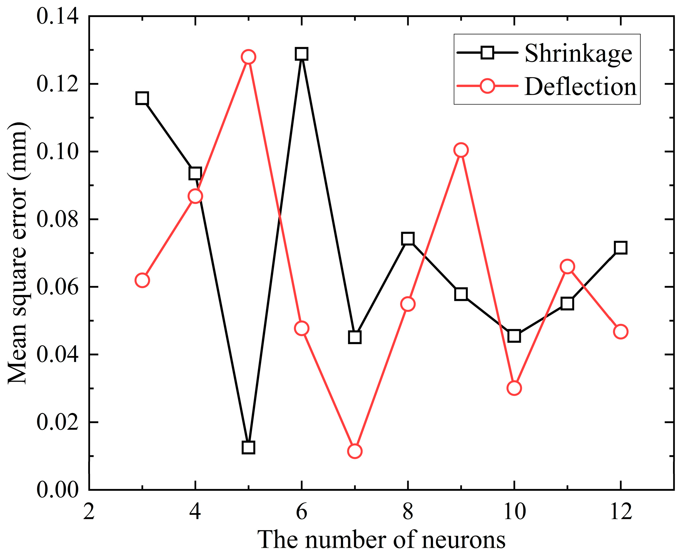
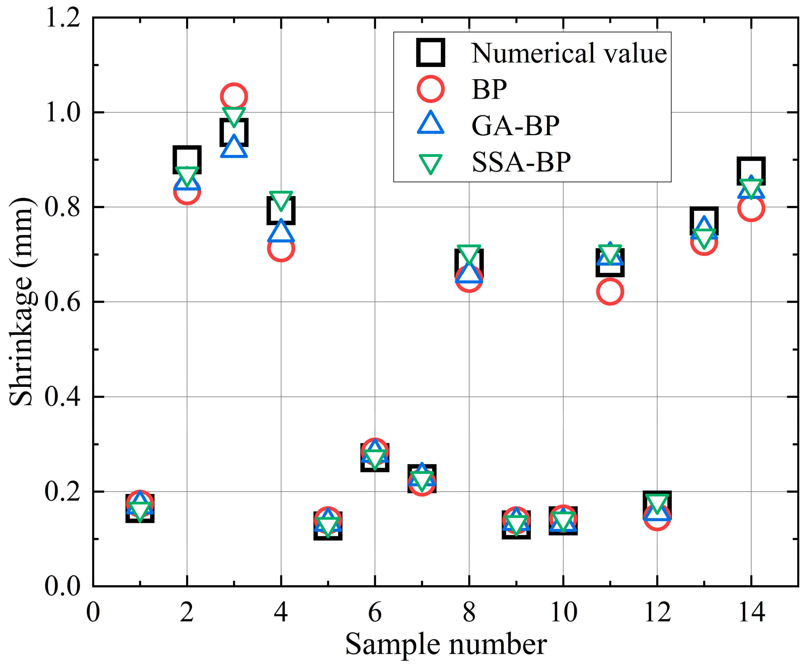
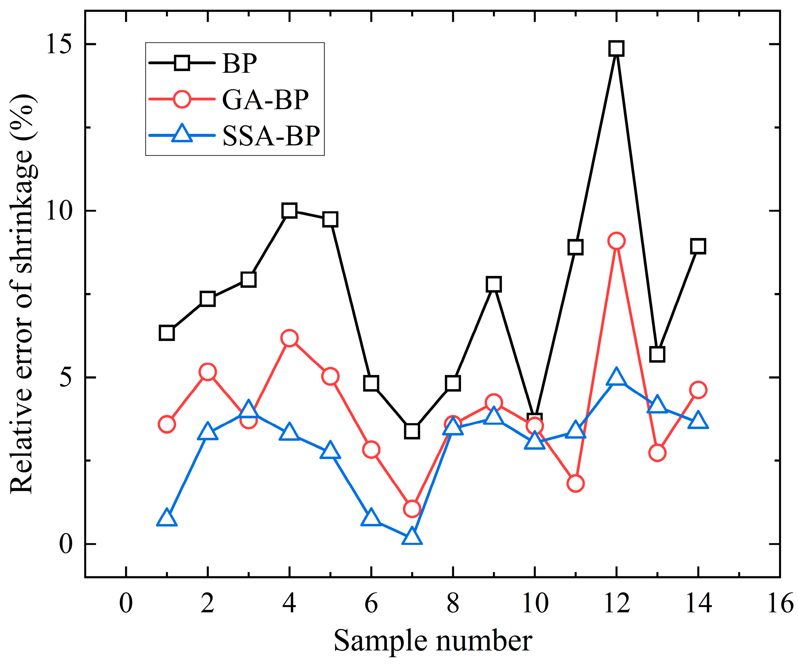
4.1. Prediction of Shrinkage

Based on the BP model, GA-BP model, and SSA-BP model, the shrinkage of 14 samples in prediction sets is predicted. The comparison between the predicted values and the numerical values of the three models is shown in Figure 20. When the BP model is applied to predict shrinkage, there is a greater absolute error between the predicted values of samples 2, 4, and 11 and the numerical values. Compared with the BP model, the GA-BP model and SSA-BP model have smaller absolute errors in predicting the shrinkage of 14 predicted samples.

The relative error between the actual values and the predicted values of the three models is shown in Figure 21. When the BP model is applied to predict the shrinkage of titanium alloy, sample 12 has the largest relative error of 14.9%. Compared to the BP model, the relative errors of the 14 predicted samples are reduced when the GA-BP model and the SSA-BP model are applied to predict shrinkage. When the GA-BP model is applied to predict shrinkage, the maximum relative error is 9.1%. When the SSA-BP model is applied to predict shrinkage, the relative error of all 14 predicted samples is within 5%.

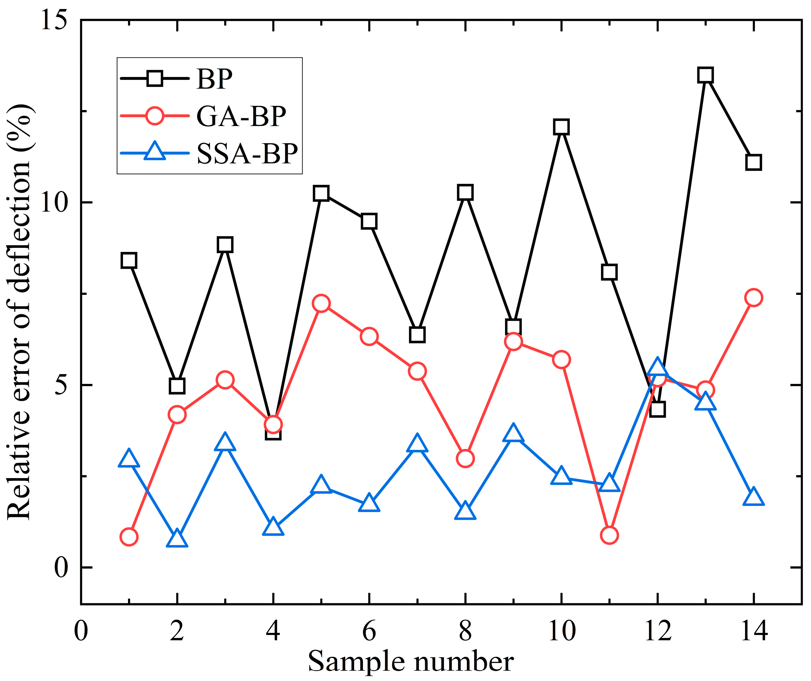
4.2. Prediction of Deflection

Based on the BP model, GA-BP model, and SSA-BP model, the deflection of 14 samples in prediction sets is predicted. The comparison between the predicted values and the numerical values of the three models is shown in Figure 22. Compared to the BP model, the predicted values of the GA-BP model and SSA-BP model are closer to the numerical values. When the BP model is applied to predict the deflection of the plate edge, there are greater absolute errors between the predicted value and the numerical value in sample 3 and sample 13.

The relative error between the predicted deflection values and the actual values of 14 predicted samples is shown in Figure 23. When the BP model is applied to predict the deflection of the edge position of the plate edge, sample 13 has the maximum relative error of 13.5%. Compared to the BP model, the relative errors of the GA-BP model and SSA-BP model are smaller in predicting the deflection of titanium alloy. When the GA-BP model is applied to predict deflection, the relative error of sample 5 is the largest, with a value of 7.2%. When the SSA-BP model is applied to predict deflection, the relative error is within 5%.

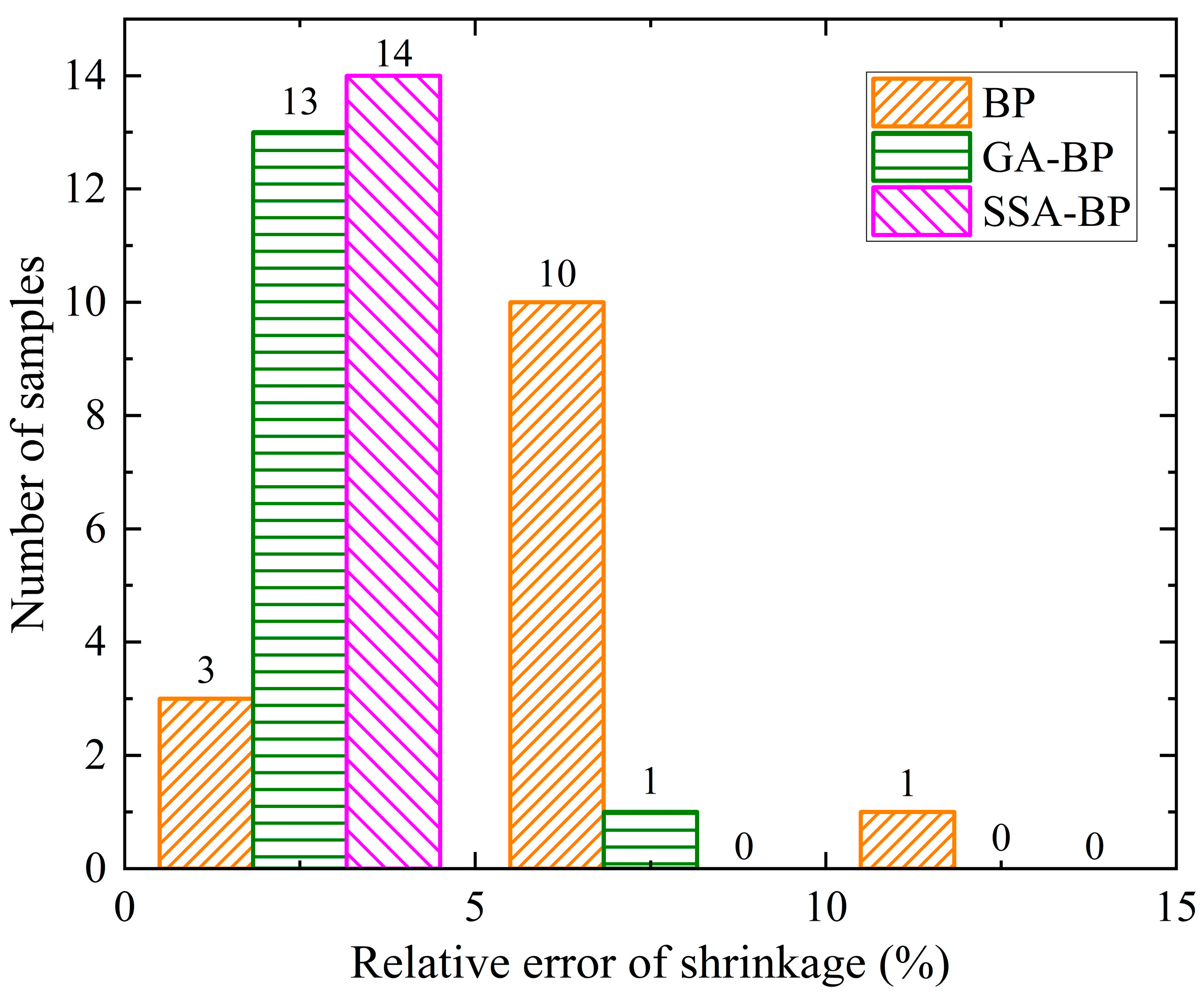
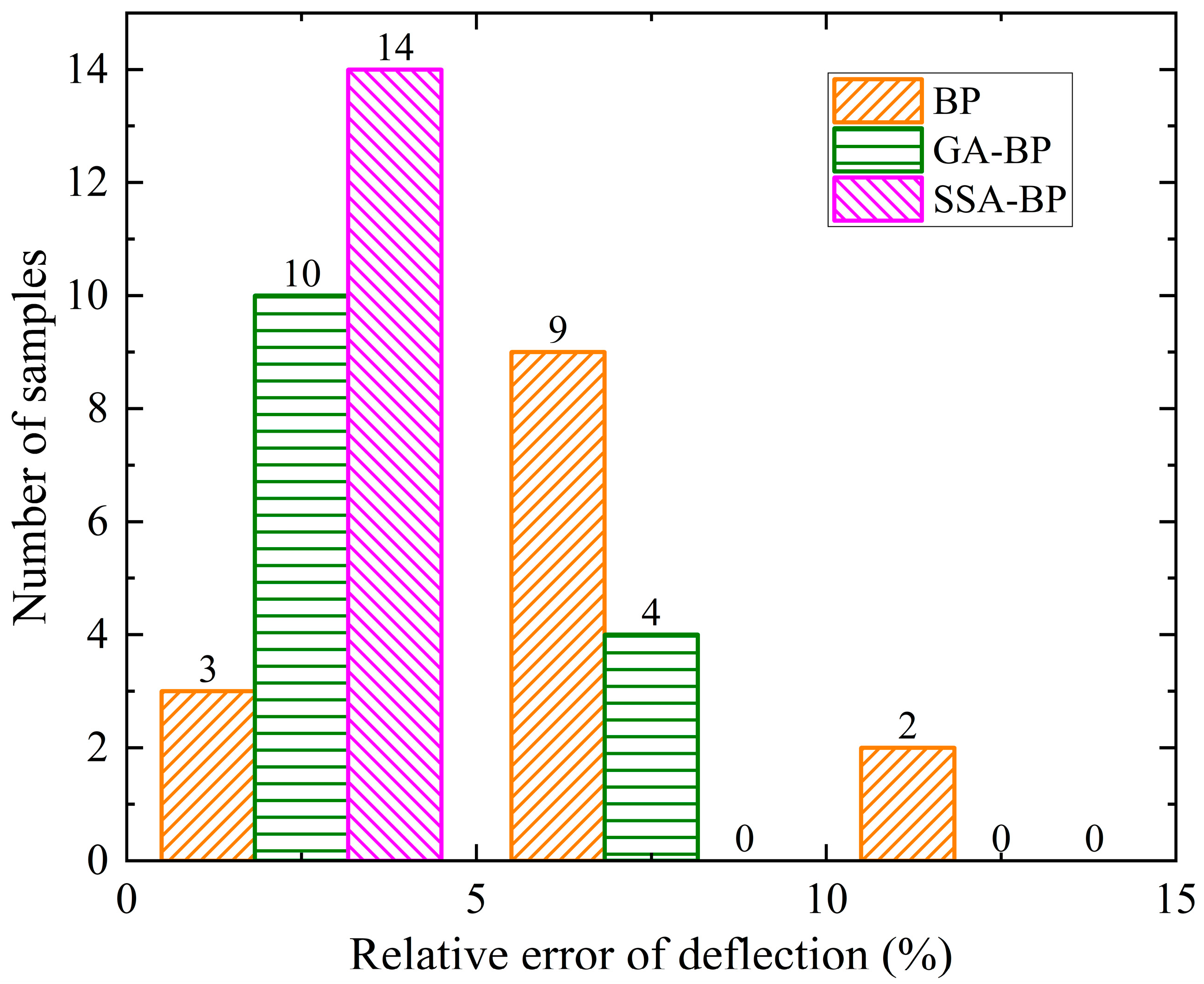
4.3. Error Distribution Statistics

After optimizing the BP neural network by the GA algorithm and SSA algorithm, the accuracy of the prediction model is improved, and the error between the predicted values and the true values is reduced. Compared to the GA-BP model, the SSA-BP model has a higher prediction accuracy. The BP model, GA-BP model, and SSA-BP model are used to predict the shrinkage of the plate edge of the titanium alloy heating line side, and the relative error distributions of the predicted samples are shown in Figure 24. For the 14 predicted samples, the BP model has three prediction samples with relative errors less than 5% and two prediction samples with relative errors greater than 10%. The GA-BP model has one predicted sample with an error greater than 5%, whereas the relative error of the remaining samples is less than 5%. Compared to the BP model and GA-BP model, the relative error of predicted samples by the SSA-BP model is all within 5%, with a more concentrated distribution.

The BP model, GA-BP model, and SSA-BP model are used to predict the deflection, and the relative error distributions of the predicted samples are shown in Figure 25. For the 14 predicted samples, the BP model has three prediction samples with relative errors less than 5% and one prediction sample with relative errors greater than 15%. The GA-BP model has one predicted sample with an error greater than 5%, whereas the relative error of the remaining samples is less than 5%. The relative error of 14 predicted samples by the SSA-BP model is all within 5%.

In addition to the MSE, R², and MAPE mentioned above, root mean square error (RMSE) and mean absolute error (MAE) can also be used to evaluate the accuracy of titanium alloy deformation prediction models. The calculation formulas for RMSE and MAE are shown in Formulas (21) and (22):

$$\mathrm{R}\mathrm{M}\mathrm{S}\mathrm{E}=\sqrt{\frac{1}{n}\sum _{i=1}^n{\left(y_i-y_i^{\prime }\right)}^2}$$

(21)

$$\mathrm{M}\mathrm{A}\mathrm{E}=\frac{1}{n}\sum _{i=1}^n\left|y_i-y_i^{\prime }\right|$$

(22)

Based on the finite element method to calculate the deformation of titanium alloy forming, the time spent for a single calculation is 16,562 s, which consumes a lot of computational resources and computational time. The BP, GA-BP, and SSA-BP model training time and prediction time are shown in

Table 6. Comparison of training time, prediction time, and numerical calculation time between models.

Types of Predictions	Types of Models	Training Time (s)	Prediction Time (s)	Total Training and Prediction Time (s)	Time for Numerical Calculation (s)
shrinkage	BP	59	1	60
	GA-BP	156	1	157	16,562
	SSA-BP	334	1	335
deflection	BP	58	1	59
	GA-BP	131	1	132	16,562
	SSA-BP	323	1	324

. The time required to train the BP model for predicting the shrinkage of titanium alloy forming is 59 s. Compared to the BP model, the GA-BP model and SSA-BP model take more time to train, which are 156 s and 334 s, respectively. The time required to train the BP, GA-BP, and SSA-BP models for predicting the deflection of titanium alloy forming is 58 s, 131 s, and 323 s, respectively. Three models were trained and used to predict the shrinkage and deflection of titanium alloy forming, with a prediction time of 1 s. Compared with a numerical simulation, the application of BP, GA-BP, and SSA-BP models to calculate the deformation of titanium alloy requires less calculation time and can quickly predict deformation.

The prediction error and accuracy evaluation of the BP, GA-BP, and SSA-BP models are shown in

Table 7. Prediction error and accuracy evaluation between models.

Predicted Variables	Prediction Models	R2	MSE (mm)	RMSE (mm)	MAE (mm)	MAPE (%)
shrinkage	BP	0.988	0.0021	0.046	0.037	7.45
	GA-BP	0.995	0.0007	0.026	0.020	4.08
	SSA-BP	0.997	0.0005	0.022	0.016	2.96
deflection	BP	0.986	0.7299	0.854	0.679	8.44
	GA-BP	0.997	0.2328	0.482	0.383	4.73
	SSA-BP	0.998	0.0762	0.276	0.205	2.64

. The R² of SSA-BP is closest to 1 among the three models. The MSE, RME, and MAE of the SSA-BP model are smaller than that of the other two prediction models. Compared with the BP model, the MAPE is reduced by 45.23% and 60.27% for predicting shrinkage through the application of the GA-BP model and the SSA-BP model, respectively. The MAPE is reduced by 43.96% and 68.72% for predicting deflection through the application of the GA-BP model and the SSA-BP model, respectively. Therefore, the prediction accuracy of the optimized BP model through the application of the SSA algorithm and GA algorithm is improved. The prediction accuracy of the SSA-BP model is better than that of the GA-BP model.

5. Conclusions

To solve the problem of deformation prediction for titanium alloy forming, the numerical calculation model of line heating for titanium alloy was established by the finite element method. The shrinkage and deflection of titanium alloy forming under different geometric and forming parameters were obtained by numerical calculations. The sample data were divided into a training set and prediction set. Based on the training set, the BP, GA-BP, and SSA-BP models were established to predict shrinkage and deflection. The prediction accuracy of the three prediction models was analyzed through the prediction set. The intelligent prediction model provides data support for intelligent decisions for titanium alloy forming.

• Compared with the forming experiment, the feasibility of the titanium alloy numerical calculation model was verified by comparing it with the numerical calculations and experimental results of low-carbon steel. The results of numerical calculations of titanium alloy can provide basic data for the prediction of titanium alloy deformation.
• To quickly predict the deformation of titanium alloy, the deformation prediction model suitable for titanium alloy forming was established based on the training set and BP neural network algorithm. The BP neural network model was optimized by the GA algorithm and SSA algorithm, and the prediction model of titanium alloy deformation by GA-BP and SSA-BP was established. The BP, GA-BP, and SSA-BP models can all be applied to predict the shrinkage and deflection for titanium alloy forming.
• BP, GA-BP, and SSA-BP models were applied to predict the deformation of titanium alloy. The MAPEs for shrinkage prediction were 7.45%, 4.08%, and 2.96%, respectively. The MAPEs in deflection prediction are 8.44%, 4.73%, and 2.64%, respectively. Therefore, the prediction accuracy of SSA-BP is higher than BP and GA-BP.
• The application of both the GA algorithm and SSA algorithm can obtain good initial weights and thresholds to avoid the BP neural network falling into a local optimal solution. The BP neural network model is optimized by the GA algorithm and SSA algorithm, which is suitable for fast and accurate prediction of deformation in titanium alloy forming.

References

1. Wang, K.; Wu, L.; Li, Y.; Sun, X. Study on the overload and dwell-fatigue property of titanium alloy in manned deep submersible. China Ocean Eng. 2020, 34, 738–745. [Google Scholar] [CrossRef]
2. Wei, B.; Zhang, F.; He, K.; Li, Z.; Du, R. Deformation and springback behavior of sheet metal with convex-shaped surfaces in heat-assisted incremental bending process based on minimum energy method. J. Manuf. Sci. Eng.-Trans. ASME 2023, 145, 031003. [Google Scholar] [CrossRef]
3. Han, X.; Zhou, B.; Tan, S. Effect of heating spacing on deformation distribution of line heating process. J. Ship Prod. Des. 2019, 35, 1–11. [Google Scholar] [CrossRef]
4. Huang, H.; Murakawa, H. Thermo-mechanical analysis of line heating process by an efficient and accurate multi-level mesh refining method. Mar. Struct. 2016, 49, 239–255. [Google Scholar] [CrossRef]
5. Vega, A.; Escobar, E.; Fong, A.; Ma, N.; Murakawa, H. Analysis and prediction of parallel effect on Inherent deformation during the line heating process. CMES-Comp. Model. Eng. Sci. 2013, 90, 197–210. [Google Scholar]
6. Wróbel, I.; Skowronek, A.; Grajcar, A. A review on hot stamping of advanced high-strength steels: Technological-metallurgical aspects and numerical simulation. Symmetry 2022, 14, 969. [Google Scholar] [CrossRef]
7. Jukić, K.; Perić, M.; Tonković, Z.; Skozrit, I.; Jarak, T. Numerical calculation of stress intensity factors for semi-elliptical surface cracks in buried-arc welded thick plates. Metals 2021, 11, 1809. [Google Scholar] [CrossRef]
8. Wang, C.; Pham, D.T.; Wu, C.; Kim, J.; Su, S.; Jin, Z. Artificial thermal strain method: A novel approach for the analysis and fast prediction of the thermal distortion. J. Mater. Process. Technol. 2021, 289, 116937. [Google Scholar] [CrossRef]
9. Wang, H.; Wang, K.; Guo, Z.; Rui, S.; Wang, Z. Resistance mechanism of partially embedded pipelines considering the influence of temperature fields. Ocean Eng. 2023, 281, 114720. [Google Scholar] [CrossRef]
10. Yi, M.; Park, J.; Seo, J. A novel pre-processing modelling method for the finite element analysis of the thermal deformation of large structures in the erection stage. Ocean Eng. 2022, 266, 112891. [Google Scholar] [CrossRef]
11. Li, F.; Jiang, J.; Wang, J.; Wang, J.; Chen, X. Experimental study and numerical simulation on springback of Ti-6Al-4V alloy under hot U-bending. J. Mech. Sci. Technol. 2023, 37, 3691–3697. [Google Scholar] [CrossRef]
12. Baffari, D.; Buffa, G.; Campanella, D.; Fratini, L.; Micari, F. Single block 3D numerical model for linear friction welding of titanium alloy. Sci. Technol. Weld. Join. 2019, 24, 130–135. [Google Scholar] [CrossRef]
13. Villa, M.; Brooks, J.W.; Turner, R.; Boitout, F.; Ward, R.M. Metallurgical modelling of Ti-6Al-4V for welding applications. Metals 2021, 11, 960. [Google Scholar] [CrossRef]
14. Sarikavak, Y. An advanced modelling to improve the prediction of thermal distribution in friction stir welding (FSW) for difficult to weld materials. J. Braz. Soc. Mech. Sci. Eng. 2021, 43, 4. [Google Scholar] [CrossRef]
15. Li, L.; Qi, S.; Zhou, H.; Wang, L. Prediction of line heating deformation on sheet metal based on an ISSA-ELM model. Sci. Rep. 2023, 13, 1252. [Google Scholar] [CrossRef] [PubMed]
16. Jonaet, A.; Park, H.; Myung, L. Prediction of residual stress and deformation based on the temperature distribution in 3D-printed parts. Int. J. Adv. Manuf. Technol. 2021, 113, 2227–2242. [Google Scholar] [CrossRef]
17. Asmael, M.; Nasir, T.; Zeeshan, Q.; Safaei, B.; Kalaf, O.; Motallebzadeh, A.; Hussain, G. Prediction of properties of friction stir spot welded joints of AA7075-T651/Ti-6Al-4V alloy using machine learning algorithms. Arch. Civ. Mech. Eng. 2022, 22, 94. [Google Scholar] [CrossRef]
18. Uz, M.; Yoruc, A.; Cokgunlu, O.; Cokgunlu, O.; Aydogan, C.; Yapici, G. A comparative study on phenomenological and artificial neural network models for high temperature flow behavior prediction in Ti6Al4V alloy. Mater. Today Commun. 2022, 33, 104933. [Google Scholar] [CrossRef]
19. Bautista-Monsalve, F.; García-Sevilla, F.; Miguel, V.; Naranjo, J.; Manjabacas, M.C. A novel machine-learning-based procedure to determine the surface finish quality of titanium alloy parts obtained by heat assisted single point incremental forming. Metals 2021, 11, 1287. [Google Scholar] [CrossRef]
20. Datta, S.; Das, A.; Raza, M.; Saha, P.; Pratihar, D. Study on laser beam butt-welding of nitinol sheet and input-output modelling using neural networks trained by metaheuristic algorithms. Mater. Today Commun. 2022, 32, 104089. [Google Scholar] [CrossRef]
21. Li, L.; Wang, J. Mathematical temperature model of sheet metal in friction stir incremental forming. Int. J. Adv. Manuf. Technol. 2019, 105, 3105–3116. [Google Scholar] [CrossRef]
22. Ji, C.M.; Hu, J.Q.; Wang, B.; Zou, Y.J.; Yang, Y.S.; Sun, Y.G. Mechanical behavior prediction of CF/PEEK-titanium hybrid laminates considering temperature effect by artificial neural network. Compos. Struct. 2021, 262, 113367. [Google Scholar] [CrossRef]
23. Zheng, Y.; Li, L.; Qian, L.; Cheng, B.; Hou, W.; Zhuang, Y. Sine-SSA-BP ship trajectory prediction based on chaotic mapping improved sparrow search algorithm. Sensors 2023, 23, 704. [Google Scholar] [CrossRef]
24. Xue, J.; Shen, B. A novel swarm intelligence optimization approach: Sparrow search algorithm. Syst. Sci. Control Eng. 2020, 8, 22–34. [Google Scholar] [CrossRef]
25. Wang, S.; Dai, J.; Wang, J.; Li, R.; Wang, J.; Xu, Z. Numerical calculation of high-strength-steel saddle plate forming suitable for lightweight construction of ships. Materials 2023, 16, 3848. [Google Scholar] [CrossRef]
26. Huang, B.; Li, C.; Shi, L.; Qiu, G. China Engineering Materials Encyclopedia; Chemical Industry Press: Beijing, China, 2006. [Google Scholar]
27. Wang, S.; Wang, J.; Liu, Y.; Li, R.; Xiao, L. Analysis of forming regularity in line heating process for curved hull plate by considering the plate deflection. J. Ship Prod. Des. 2019, 35, 211–219. [Google Scholar] [CrossRef]
Figure 1. The process of titanium alloy line heating.
Jmse 12 00255 g001
Figure 2. Forming process of titanium alloy double-curved hull plate.
Jmse 12 00255 g002
Figure 3. The sketch map of line heating forming.
Jmse 12 00255 g003
Figure 4. The heating line position and grid division of the numerical calculation model of titanium alloy line heating.
Jmse 12 00255 g004
Figure 5. The influence of different mesh size on temperature.
Jmse 12 00255 g005
Figure 6. Shrinkage and deflection of low-carbon steel with different mesh sizes.
Jmse 12 00255 g006
Figure 7. Shrinkage and deflection of titanium alloy under different mesh sizes.
Jmse 12 00255 g007
Figure 8. Constraint diagram of a numerical calculation model of titanium alloy line heating.
Jmse 12 00255 g008
Figure 9. Numerical calculation process of titanium alloy line heating.
Jmse 12 00255 g009
Figure 10. The law of the maximum temperature of titanium alloy and low-carbon steel along the heating line.
Jmse 12 00255 g010
Figure 11. Experimental measurement and numerical simulation of deformation field of low-carbon steel: (a) the shrinkage along the heating line; (b) the deflection of the edge of the heating line side.
Jmse 12 00255 g011
Figure 12. Comparison of deformation field between titanium alloy and low-carbon steel: (a) shrinkage; (b) deflection.
Jmse 12 00255 g012
Figure 13. Comparison of temperature field and deformation field at plate edge of the titanium alloy heating line side: (a) shrinkage and temperature; (b) deflection and temperature.
Jmse 12 00255 g013
Figure 14. Sample distribution of two-variable and three-variable Latin hypercube sampling: (a) two-variable; (b) three-variable.
Jmse 12 00255 g014
Figure 15. BP neural network structure of titanium alloy-forming deformation prediction.
Jmse 12 00255 g015
Figure 16. Mean square error of hidden layer with a different number of neurons.
Jmse 12 00255 g016
Figure 17. R2 and MAPE under different optimization schemes.
Jmse 12 00255 g017
Figure 18. GA-BP neural network training process.
Jmse 12 00255 g018
Figure 19. SSA-BP neural network training process.
Jmse 12 00255 g019
Figure 20. Comparison between predicted values and numerical values of shrinkage.
Jmse 12 00255 g020
Figure 21. Comparison of relative errors in shrinkage prediction models.
Jmse 12 00255 g021
Figure 22. Comparison between predicted values and numerical values of deflection.
Jmse 12 00255 g022
Figure 23. Comparison of relative errors in deflection prediction models.
Jmse 12 00255 g023
Figure 24. Error distribution of shrinkage prediction model.
Jmse 12 00255 g024
Figure 25. Error distribution of deflection prediction model.
Jmse 12 00255 g025