Abstract
The accurate generation of a target sea state in numerical or experimental wave tanks is a fundamental line of research for the ocean engineering community. It guarantees the quality and relevance of wave–structure interaction tests. This study presents a reproducible irregular wave generation and qualification procedure, accounting for the nonlinear aspects of wave propagation. It can be used for both numerical simulation and experiments. The presented numerical and experimental results are obtained from the OpenFOAM solver and the Ecole Centrale Nantes wave tank facilities, respectively. The procedure comprises two steps: First, the wavemaker motion is calibrated numerically to generate the target wave spectrum at the position of interest. This is achieved with a wavemaker-equipped nonlinear potential flow solver. The open-source HOS-NWT solver, based on the high-order spectral method, was employed in this study. Then, the corrected wavemaker motion is used directly in the experimental wave tank. OpenFOAM simulations were performed to generate waves with the relaxation method, using wave elevation and velocity field data from HOS-NWT. The procedure was finally tested for mild and extreme breaking sea states. The waves generated by the HOS-NWT solver, the experiment, and the OpenFOAM simulation were compared from both stochastic and deterministic perspectives.
1. Introduction
Floating bodies operating in the ocean encounter various environmental conditions throughout their lifetime, including wind, currents, and waves. The primary load on the floating bodies is induced by waves in the ocean. Wave–structure interaction (WSI) is a major concern in the design of ship and marine structures. Many academic and industrial actors have conducted wave basin experiments or computational fluid dynamics (CFD) simulations to test WSI performances [1,2,3,4]. The waves generated for these tests must accurately represent specific in situ wave conditions and be easily reproduced in both an experimental wave tank (EWT) and CFD-based numerical wave tank (CFD-NWT). Therefore, it is essential for WSI tests to establish a uniform procedure to reproduce accurately irregular wave fields for both EWTs and NWTs. This procedure should accurately generate the target sea state at the location of interest within the domain and ensure the quality of the wave corresponding waves.
In the EWT wave generation procedure, the wavemaker motions are typically constructed using a linear transfer function applied to the target wave spectrum with random phases. However, the natural nonlinear characteristics of waves lead to changes in their statistical properties as they propagate from the wavemaker. Furthermore, replicating a specific target wave, such as a wave field generated by a numerical code, using a linear transfer function is a complex challenge.
In the case of a CFD-NWT simulation, mainly three wave generation approaches can be considered. The first approach is the modeling of a moving wavemaker, where the CFD solver generates and propagates waves by manipulating the wavemaker’s stroke. While this method can replicate experimental waves in an NWT, it requires significant computational resources to model the whole wave tank, including the wavemaker. The second approach is a inner-domain wave-making method [5], which can model the propagation of the intermediate and shallow water waves using a Boussinesq-type model [6,7]. The third approach imposes the velocity and elevation of the incident wave on a specific boundary or region of a smaller-size CFD domain, facilitating the efficient generation of a target incident wave. This approach is widely used in various NWT applications, such as NWT simulations of semisubmersible [8]. This approach allows the simulation of nonlinear wave interaction, such as wave breaking, in the CFD domain while maintaining efficiency by minimizing the computational domain.
As the waves propagate along the tank, the shape and parameters of the wave spectrum are affected by nonlinear wave interaction and dissipation phenomena. These effects have been extensively studied experimentally [9,10] and theoretically [11,12] in recent years. Therefore, for both EWTs and NWTs, to ensure the accurate generation of a specific sea state at the position of interest, a wave qualification procedure is essential. The latter mainly relies on two features/parameters/measures: the wave spectrum at the target location is compared with the design wave spectrum, and the wave crest height distribution, which represents the severity of the wave field, is compared with semiempirical references. On this ground, the irregular wave generation procedure includes a wave calibration step that ensures the quality of the spectrum at the target position. This calibration consists of iterative correction of the wave input (such as the wavemaker motion) to balance the wave propagation effects from the wavemaker to the target position. For the EWT, this wave calibration step is highly time-consuming and may require up to a quarter of the total experimental time. For the CFD-NWT, this procedure is almost impossible to apply because of its prohibitive computational cost.
Therefore, there is a need for alternative methods for wave calibration. In the recommended procedures and guidelines of the International Towing Tank Conference (ITTC) for the laboratory modeling of waves [13], various nonlinear irregular wave modeling methods were reviewed. From those methods, the high-order spectral (HOS) method was chosen to be employed in this study. The HOS method is a nonlinear wave generation method that can be extended up to an arbitrary order [14,15], with the advantage of being computationally efficient. In this study, we used the open source HOS-NWT program [16], which is an extension of the HOS method designed to replicate waves in an NWT using a wavemaker. The HOS-NWT solver includes all the necessary nonlinear wave propagation features and is relatively cost-effective. Furthermore, the iterative correction of the wave spectrum within such an NWT was successfully validated in previous studies [17].
The present study aimed to build and validate an irregular wave generation and qualification procedure for irregular wave experiments and CFD simulations based on an iterative HOS-NWT calibration. This procedure enables the generation and propagation of the same qualified nonlinear irregular waves in both EWTs and CFD-NWTs without a calibration process. It was expected to not only reduce the time required for experimental wave calibration but also to facilitate easy synchronization of the experimental results with the CFD-NWT results. Detailed information about and the validation of the suggested procedure in the present paper are organized as follows:
- Section 2 presents the target wave conditions used in the wave generation and qualification procedure. A strong wave breaking condition is included to assess the limitations of the suggested procedure;
- Section 3 presents the wave generation and qualification procedure and workflow of the present study. The deterministic and stochastic comparison approaches are also introduced;
- Section 4 presents details on the iterative wave calibration procedure using the HOS-NWT solver. The iteration with the error criterion is applied to obtain an appropriate wave spectra in the numerics;
- Section 5 describes the experimental setup in the École Centrale Nantes (ECN) Ocean Engineering tank;
- Section 6 details the numerical features of the OpenFOAM simulations, the wave generation methodology, and validation with spatial and temporal refinement;
- Section 7 gives a comparative analysis between the HOS-NWT, the experiment, and the CFD simulation. Deterministic analyses were performed by comparing the wave elevation and the wave profile during wave breaking events. Stochastic quantities such as the wave spectrum and the crest probability of exceedance were also compared;
- Section 8 provides a summary of the wave generation and qualification procedures, the limitations of the study, and our future plans.
2. Wave Conditions
In this study, the suggested procedure was applied to two design sea states, named Case1 and Case3. These sea states are the same as the wave conditions considered during the “Reproducible Offshore CFD” joint industrial project [18], which has been conducted by various academic and industrial groups. For both cases, the design wave spectra follow the unidirectional Joint North Sea Wave Project (JONSWAP) model [19].
Table 1 presents the JONSWAP parameters for Case1 and Case3. The significant wave height is denoted as , the peak period as , the peak wavelength as , the magnification factor as , and the steepness parameter as . The Benjamin–Feir Index (BFI) parameter, characterizing the nonlinear wave interactions (also known as Benjamin-Feir instability), was estimated using the formula suggested by Serio et al. [20].

Table 1.
Irregular wave parameters based on the JONSWAP spectrum.
The normalized spectrum shapes of Case1 and Case3 are depicted in Figure 1. Both wave conditions can be assumed to be deep-water conditions. Case3 corresponds to the Gulf of Mexico 1000-year return period sea state, where frequent and intense wave breaking events are expected, and Case1 represents a relatively mild sea state, where wave breaking barely occurs.
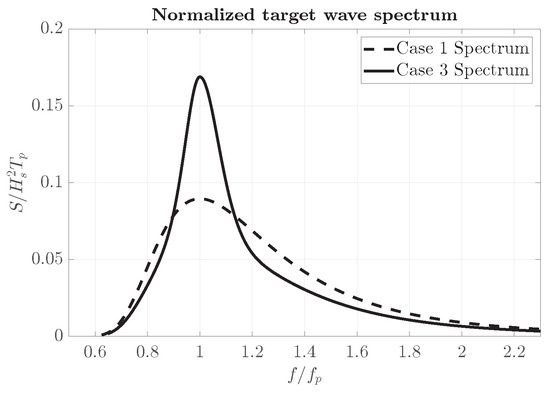
Figure 1.
Normalized target wave spectra for Case1 and Case3.
3. Wave Generation and Qualification
Generating consistent irregular waves for WSI tests, in both experimental and numerical studies, presents challenges owing to the nonlinearity of the waves. The target sea state has to be generated at a given distance from the wavemaker denoted and denoted the target location. In severe sea states, the stochastic properties of the wave field evolve with propagating distance, primarily due to nonlinear wave interactions and energy dissipation. Therefore, a procedure to accurately reproduce a designated wave field, satisfying both stochastic and deterministic criteria, at the target location is essential. The following sections introduce a data analysis methodology and an algorithm designed to reproduce nonlinear waves in both the experimental wave tank and the CFD-NWT.
3.1. Metrics for the Data Analysis
The metrics for the wave qualification procedure fulfill two distinct objectives: first, to evaluate the similarity between two temporal wave measurements for a deterministic comparison; and second, to compare the stochastic characteristics of different sea states.
3.1.1. Deterministic Comparison
When the free surface elevation is provided as spatio-temporal information, a relative difference function in Equation (1) can be introduced to observe the time-varying difference.
where is the reference wave height that is chosen to be the significant wave height for irregular waves, N is the number of measurement locations along the propagation, and and are the wave elevations compared. Furthermore, the averaged Pearson correlation coefficient can be considered with a moving time window [21].
where represents the local Pearson correlation coefficient of each elevation measurement is given as:
where represents the covariance of data p and q, is the standard deviation of data q, and represents the time window duration. In the present study, was chosen following Choi et al. [22]. With this approach, the time shift () from the reference run (maximizing the cross correlation) is computed to estimate a time-dependent deterministic error. Therefore, the time shift () and the averaged Pearson correlation coefficient () are compared.
3.1.2. Stochastic Comparison
The wave spectrum is evaluated using Welch’s spectral density estimation method with a smoothing window length of for each realization [23]. Each spectrum can be bounded by a confidence interval, which accounts for the sample variability of the data. The spectra are then averaged over the N realizations to obtain the averaged spectrum .
The stochastic properties of waves, such as the significant wave height , are evaluated from the wave spectrum. The wave peak frequency is evaluated using the Young [24] technique.
The probability distribution of the wave crest heights from single realizations (PDSR) and the ensemble realization (PDER) is also considered. Since different wave realizations give different wave crest PDSR curves, Huang and Zhang [25] proposed the PDSR range with a confidence level. The PDER is evaluated for N realizations to include all events. For the analysis of PDER, the Jeffrey confidence intervals [26] are also utilized to estimate the sampling variability error. For this analysis, the uncertainty limit was set at the probability of the 20th most extreme event.
3.2. Wave Qualification Criteria
Criteria for qualifying the spectrum and crest height distributions were established in the ‘Reproducible CFD modeling Practice for Offshore Applications’ Joint Industrial Project [18].
According to these criteria, a generated sea state is considered qualified if the relative spectrum error (), as defined in Equation (5), remains within of the target frequency range , where is the wave peak frequency of the sea state.
where is the measured wave spectrum from EWT, HOS-NWT, and CFD-NWT, and is the target wave spectrum.
The probability distribution of the wave crest height is also used for wave qualification. The measured PDSR and PDER are compared with reference wave crest height distributions. Longuet-Higgins [27] showed that the wave crest distribution of linear waves with assumptions of a Gaussian distribution and a narrow-band spectrum follows the Rayleigh distribution. However, the Rayleigh distribution is known to underestimate the height of the wave crests, particularly in severe sea states. Forristall [28] suggested the wave crest distribution based on second-order theory. Later, Huang and Zhang [25] proposed a semiempirical formula for the PDER curve and the mean and 99% upper and lower bounds of the PDSR curves, derived from the numerical wave simulation of 305 sea states. Therefore, the Rayleigh distribution, Forristall distribution, Huang’s PDER distribution, and the mean and 99% bounds of Huang’s distributions were used as references for comparing the measured PDSR and PDER curves. However, studies such as Onorato et al. [29] and Canard et al. [30] showed that, in a wave tank environment, the distribution of the wave crest heights depends mainly on the distance from the wavemaker due to modulational instabilities that develop during the propagation of unidirectional irregular sea states. The references mentioned above are dedicated to open ocean description and consequently do not consider these effects and, thus, should be used carefully.
3.3. Available Tools and Adopted Procedure
Obtaining converged wave stochastic properties in experiments or CFD simulations is extremely time-consuming because a significant number of realizations of irregular waves are required. Additionally, proposing a calibration procedure in EWTs or CFD-NWTs will be highly time-consuming, making it practically unusable. Therefore, a dedicated and efficient numerical wave tank tool based on potential flow theory can be used in a preliminary step.
To this end, this study proposes a novel wave calibration and generation procedure that employs the HOS-NWT solver as an iterative wave calibration tool. This will provide the adequate wavemaker motion for EWTs and/or the nonlinear incident wave field for CFD-NWTs. Figure 2 illustrates the workflow of irregular wave calibration and generation.
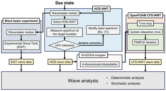
Figure 2.
Wave generation and qualification workflow for the HOS-NWT, the wave basin experiment, and the OpenFOAM simulations.
When the target sea state is chosen, the iterative wave calibration process is performed with the HOS-NWT solver (see Section 4 for details). The wavemaker motion in the HOS model is adjusted iteratively, continuing until the relative difference in the wave spectrum ( in Equation (5)) falls within a tolerance. After the iteration procedure is completed, the wavemaker motions for the EWT and the HOS wave data for the CFD-NWT are available to conduct the WSI study of interest. One objective of the present study was, thus, to perform the wave qualification process with the waves measured experimentally and the ones computed with the CFD-NWT (see Section 7). Finally, the wave qualification process is performed for the waves measured from the experiment and the CFD simulation.
4. Iterative Wave Calibration with HOS-NWT
The HOS-NWT solver, which is an extension of the HOS method, incorporates specific features of a wave tank environment, such as a wavemaker, lateral reflective walls, and an absorbing beach. It has been extensively validated and used as a digital twin of the ECN wave basin.
The nonlinear potential flow models naturally neglect vorticity and viscosity effects by employing irrotational and inviscid assumptions, which dramatically facilitate the wave modeling. However, these assumptions prevent the use of potential flow solvers for phenomena involving strong viscous effects or high vorticity such as breaking waves. To overcome this limitation, the Tian–Barthelemy wave breaking model was employed. This model uses Tian’s eddy viscosity model with Barthelemy’s breaking criterion [31,32]. The wave breaking model predicts the onset of wave breaking events and estimates the amount of dissipation using the wave profile.
Calibration at the Target Position Using HOS-NWT
The preliminary step of generating calibrated HOS-NWT waves for sea states Case1 and Case3 was performed using an iterative procedure. As the detailed process of this iterative wave calibration using HOS-NWT is thoroughly described in Canard et al. [17], this section will briefly outline the numerical setup of the HOS-NWT solver.
The 2D numerical domain (length, depth, and wavemaker geometry) was set to mimic the ECN Ocean Engineering wave tank to allow consistent comparisons with the experiment. The dimensions of the 2D numerical wave tank were m in length and m in depth. The target location from the mean wavemaker was set to 708 m (i.e., ) for Case1 and 750 m (i.e., ) for Case3. Note that the numerical absorbing beach was tuned to minimize wave reflection.
Table 2 presents the HOS-NWT numerical setup adopted for Case1 and Case3. Spatial discretization was specified using , i.e., the largest wave number solved, which is related to the number of nodes in the x direction (). is the number of HOS nodes in the vertical direction. The HOS simulation time () for each seed was 10,800 s, excluding the transitory stage for wave propagation. The wave breaking model was activated only for Case3. The intensity of the eddy viscosity (), introduced for the wave breaking model in Tian et al. [31], acted as the damping when the wave breaking event occurred. For this study, was used. Finally, the HOS order was set to , which ensured an accurate and efficient solution of the nonlinear problem.
Table 2.
HOS-NWT numerical setup for Case1 and Case3.
The iterative spectrum correction procedure was applied to Case1 and Case3 at their respective target locations. Following the calibration procedure in Canard et al. [17], after 1 and 4 iterations for Case1 and Case3, respectively, the mean wave spectrum at satisfied the criterion. In Canard et al. [17], 100 realizations per sea state were calibrated. Since such a large number of realizations cannot be performed in CFD or in experiments, for the present study, we used selected 10 realizations for each sea state.
Figure 3 presents the Case3 wave spectrum and the crest ensemble distribution computed using the 100 seeds (left plots), and the 10 seeds selected for CFD and experimental reproduction (right plots). The thick solid black line, which is the mean wave spectrum, satisfies the criterion. The gray lines in the spectrum plots correspond to the spectra computed from the individual realizations. The confidence intervals are also displayed to quantify the increase in the sampling variability error that follows the selection of the 10 seeds.
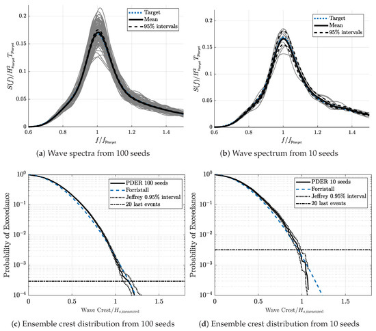
Figure 3.
Case3 HOS-NWT wave spectra and ensemble crest distribution at after iteration, using the 100 seeds (a,c), and the 10 seeds selected for CFD and experimental reproduction (b,d). The grey lines in the spectrum plots correspond to the spectra computed from the individual realizations.
5. Experiments in ECN Ocean Wave Tank
The wave generation experiments, following the workflow in Figure 2, were conducted in the ECN Ocean Engineering tank. In these experiments, the calibrated wavemaker motion derived from the iterative procedure using the HOS-NWT solver was applied to the experimental wavemaker. For both sea states Case1 and Case3, 10 realizations were reproduced in the wave tank.
This section briefly describes the experimental setup, and the experimental results are discussed in Section 7. Further details on the wave basin experiments can be found in Canard et al. [33].
Experimental Setup
Figure 4 presents the dimensions of the ECN Ocean Engineering tank, which measures 46.4 m in length, 29.74 m in width, and 5 m in depth. The tank features a segmented wavemaker at one end, consisting of 48 independent flaps with hinges positioned 2.147 m above the bottom. At the opposite end of the tank, a parabolic absorbing beach is installed to reduce wave reflections, limiting the reflection to under 5% of the wave amplitude for the range of wave frequencies considered for the present study.
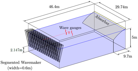
Figure 4.
ECN ocean engineering tank dimensions.
To use optimized wavemaker capabilities and position the target near the middle of the wave tank, the waves for Case1 and Case3 were generated on a scale of 1:40 and 1:50, respectively. The tank was equipped with resistive wave gauges measuring the free surface elevation time series with a sampling frequency of 100 Hz. The uncertainty tests for the same wave measurement system were conducted in Canard et al. [30], and the uncertainty of corrected calibration factor of the wave gauge was about 2.5% in the calibration stage. The positions of these gauges, both in the model and full-scale, are listed in Table 3. WG1, positioned at the target location, was the reference wave gauge for the experiment. WG4 and WG5, installed for validation purposes, were placed at the same distance from the wavemaker along a transversal line.
Table 3.
The position of wave gauges in the x-direction from the wavemaker in the ocean engineering tank. WG1 was the reference wave gauge.
6. CFD Simulations with the OpenFOAM foamStar Solver
This study employed Open-source Field Operation And Manipulation (OpenFOAM) [34] as a CFD tool. OpenFOAM provides a C toolbox for the development of user-customized numerical solvers with pre-/postprocessing utilities, mainly for fluid mechanics solutions.
In this study, the OpenFOAM simulation was performed with an additional in-house code package, foamStar, co-developed by Bureau Veritas and ECN, which supports specific functionalities for naval applications such as wave generation and floating body controls. It also interacts with an external library, Grid2Grid, which is a wrapper program that reconstructs and interpolates the HOS-NWT wave elevations to any point where it is needed in the CFD domain following the protocol given by Choi et al. [22]. Details of the OpenFOAM formulation can be found in Seng [35], and the numerical configurations for the CFD simulation are briefly discussed.
6.1. Numerical Configurations
The governing equations were solved with a finite volume method (FVM) using an unstructured polyhedral volume mesh with appropriate spatial and temporal schemes and boundary conditions. OpenFOAM supports numerous user-selectable spatial and temporal schemes. The simulation results were sensitive to the selection of numerical schemes, especially convection and time-integration schemes. For all simulations in this study, the set of spatial discretization schemes outlined in Table 4 was used.
Table 4.
Spatial discretization schemes.
For the Reynolds-averaged Navier–Stokes equations (RANSE) simulation based on the FVM in the naval engineering field, k- SST models are widely used. However, in the OpenFOAM community, it is known that the k- SST model generates a nonphysical high viscosity beneath the free surface in two-phase flow simulations. This excessive turbulence viscosity dramatically dampens the waves within a few wavelengths, which is unrealistic in wave propagation. To avoid nonphysical damping due to the turbulence model, Larsen and Fuhrman [36] introduced a buoyancy production term for two-phase flow applications. The current work adopted this concept to address the variation in density of the two-phase flow near the free surface, naming the adopted model the ‘free surface k- SST’. In the application of the free surface k- SST model, the selection of the convection scheme is crucial for the stability and computational efficiency of the simulation, due to the mass flux in the convection term. Therefore, the first-order Gauss upwind scheme was employed for both turbulence convection terms.
The simulations were conducted using the 0.99 off-centered Crank–Nicolson scheme, identified as the most efficient time-integration scheme for wave simulation in a previous study [37]. For turbulence transport, however, the implicit Euler time-integration scheme was employed to enhance numerical stability. Eight PIMPLE iterations and four PISO iterations were utilized to minimize the error from nonlinear iterations. Since the meshes were fully orthogonal, no nonorthogonal corrector was used.
6.2. Wave Relaxation Method
An explicit relaxation method [35,38] was adapted to generate and absorb waves. It smoothly blends the computed solution with the target solution in a relaxation zone. The computed solution () is blended with the target solution (incident wave) () as shown in Equation (6). An exponential blending weight function (w) was employed that varies between 0 and 1, with the normalized coordinate of changing in the relaxation zone.
6.3. CFD Numerical Domain and Spatial Discretization
The CFD numerical domain and the numerical configuration employed for wave simulations are detailed here. Figure 5 provides a full-scale representation of the 2D rectangular NWT for numerical simulations. The CFD simulation was conducted with the model scale (1/100). However, for consistency, all values are given in full-scale terms. For a clear definition of each solver’s numerical setup, two distinct coordinate systems were introduced: one for the HOS domain and another for the CFD domain. The origin of the HOS coordinate system was established at the mean position of the wavemaker and the mean free surface. The length of the CFD domain was 1200 m and was positioned in the middle of the HOS computation domain from m to m. In addition, the water depth was 500 m. Both inlet and outlet relaxation zone lengths were set to 300 m regions, and a 600 m long CFD zone was used for pure wave propagation.
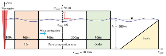
Figure 5.
Schematic view of the HOS and CFD domains for irregular wave simulation.
At the initial time (, the wave elevation and velocity were initialized across the entire CFD domain. The VOF (volume of fluid) field was set based on the HOS wave elevation, and the fluid velocity beneath the free surface was derived from the HOS wave velocity. To maximize efficiency on a multinode computer cluster system, the 3 h sequence was divided into seven or eight intervals. In each interval, 10 peak periods () overlapped with the preceding and subsequent runs. Table 5 outlines the start time () and the end time () of each interval. Each interval corresponds to 110 peak periods: 1225 s for Case1 and 1550 s for Case3. The total simulation time () was 9922.5 s for Case1 and 10,650 s for Case3. The validation of this approach is provided in Section 7.
Table 5.
Time intervals of the irregular wave simulations for Case1 and Case3 in full-scale.
Table 6 provides a summary of the mesh refinement parameters selected for each sea state. The cell sizes in the free surface refinement region are denoted as and in horizontal and vertical directions, respectively. A constant cell aspect ratio () was used. The free surface refinement region was defined between and . The upper and lower refinement zones were linearly stretched from cell sizes comparable to those of the free surface refinement zone to large cells at the top and bottom domain boundaries. The first two refinement parameters in the table refer to the reference setup. Considering that the target frequency range was , the number of cells per shortest target wavelength () was approximately for Case1 and for Case3. The computational cost of single Case3 simulation was about 120 CPU hours. The lower two mesh refinements setup in Table 6 were only used for the wave breaking event convergence test.
Table 6.
Mesh refinement parameters in full-scale for the free surface refinement region (). The upper two refinements were the reference setup for the irregular wave simulations.
7. Results and Discussion
As presented in Figure 2, this section provides a comparative analysis of the results obtained from the HOS-NWT, OpenFOAM (foamStar), and experimental data. The experimental results are briefly described, and the results of the deterministic analysis and stochastic analysis are presented. The deterministic analysis emphasizes how the time series differed when comparing the three types of results. Specific attention was paid to the time and space where the wave breaking events were identified using the HOS-NWT wave breaking model and the possible differences that can be observed in the CFD and the experiments. The stochastic analysis focuses on a spectral analysis of wave signals corresponding to a calibrated wave condition and the probability distribution on the wave crest height (PDSR and PDER).
7.1. Experimental Result
In the analysis of the experimental data, considerable attention was paid to the evaluation of the accuracy and uncertainties of the experimental process and results. The following results briefly provide an estimate of errors that affect both deterministic and stochastic variables of interest. For more comprehensive details on this experiment, the readers are referred to the work of Canard et al. [33].
7.1.1. Repeatability
During the experimental campaign, the sea state Case1 Seed1 experiment was conducted daily to test repeatability. This process resulted in eight runs and all runs started under calm water conditions, with the exceptions of Test1 and Test4, which were started just after a previous run to assess the influence of preliminary noise in the tank.
Figure 6 offers a deterministic comparison of the eight runs. The first plot in the figure presents the comparison of the time series. The second and third graphs present the comparison of the time shift () varying throughout the runs to maximize the Pearson correlation coefficient, and Test6 was chosen as the reference data. For the runs that started in calm water and over the displayed time window, the correlation was around 0.99, and the time shift was below . The errors increased for the other two runs (Test1 and Test4), providing insight into the deterioration of the waves due to the influence of preliminary noise.
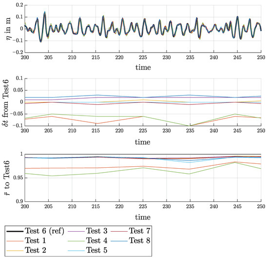
Figure 6.
Deterministic comparison among the 8 runs of the repeatability data set (Case1 Seed1), WG1 measurements.
7.1.2. Transverse Measurements
The waves measured from WG1, WG4, and WG5 were compared to verify the unidirectionality of the generated waves and quantify the possible generation of spurious transverse waves. Figure 7 displays the mean spectrum and wave crest height PDER for Case1, as measured by the three wave gauges. It is observed that the PDERs were nearly indistinguishable up to the sampling variability limit. However, the spectra present notable differences. While WG1 and WG5 showed similar results, the WG4 measurements clearly deviated from the other two wave gauges, which reached around . This deviation was most likely due to the transverse waves, which are almost unavoidable in a wave basin experiment. Since WG1 was the reference wave gauge of the experiment, hereafter, only the experiment results of WG1 are discussed.
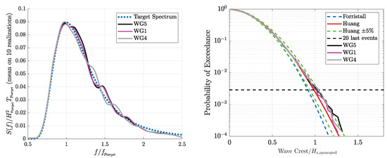
Figure 7.
Case1 wave spectrum and wave crest height PDER measured by the three wave gauges at with different lateral positions.
7.2. Deterministic Analysis
7.2.1. Influence of the Initial Time in the CFD-NWT Simulation
A notable advantage of this wave generation procedure for the CFD-NWT is that the user can choose the start time of the CFD simulation. Although performing a long CFD-NWT simulation is important for validating the proposed workflow, this approach remains beneficial since the appropriate length of the CFD simulation might be shorter than the typical 3 h realization.
This approach raises two key questions: First, how much transient time is needed for the CFD to evolve its own solution from the flow input? Second, are there accumulation errors or dysfunctions of the absorption capabilities that make the solution depend on the total simulation time? To answer these questions, the split simulations, as detailed in Table 5, were compared with a 3 h simulation.
A difference indicator function in Equation (1) was used to clearly observe the discrepancy of waves between the computational setups. Here, the reference wave elevation was the HOS-NWT, and the CFD-NWT waves were compared. The difference indicator function measures the normalized difference between the HOS-NWT wave elevation and the CFD wave elevation in the pure CFD computational ().
In Figure 8, the wave elevation from the 3 h simulations is compared to the split simulation for the test cases Case1 Seed1 Run8 and Case3 Seed5 Run7, which are the last time intervals, as described in Table 5. The computational setups for the split and 3 h simulations were identical. The first and third panels of Figure 8 display the normalized wave time series at m for Case1 and Case3, while the second and fourth panels illustrate the difference indicator function over time for the same cases. In the graphs, solid green lines represent the results of the split simulations, while orange dashed lines depict the results from the 3 h simulations. The solid blue line in the first and third panels indicates the wave elevation discrepancy between the foamStar 3 h simulations and the split simulation. For both Case1 and Case3, the time series of the wave elevation between the split and the 3 h simulations generally showed good agreement.
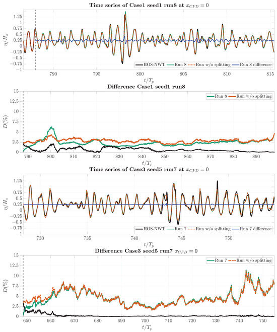
Figure 8.
Comparison between split and simulation result for Case1 Seed1 run8 (upper two plots) and Case3 Seed5 Run7 (lower two plots). The black solid line in the second and fourth panels present the discrepancy ratio between the two respective difference functions.
The solid black line shows the discrepancy ratio between two respective difference functions. For Case1, the discrepancy ratio remained below 2.5% and gradually decreased as the simulation progressed. For Case3, the discrepancy ratio between two respective difference functions slowly decreased after 20 wave peak periods. These results suggest that, while CFD-NWT and HOS-NWT may produce locally varying time series due to different approaches in modeling nonlinearities, particularly wave breaking, the impact of memory effects in CFD computations appeared to be minimal. In conclusion, both the split and the 3 h simulation methods are effective for long irregular wave simulations, although further investigation is required to clarify the minor differences observed between these two approaches, particularly in Case1.
7.2.2. Comparative Analysis of HOS-NWT, CFD-NWT, and EWT Focusing on Wave Breaking Events
A deterministic analysis of the wave elevation time series during wave breaking events was performed using both experimental and numerical results. The analysis was performed for the test case Case3 Seed6 Run4.
The timing and locations of wave breaking events were initially checked to facilitate further analysis. Figure 9 shows the wave breaking events identified using the Tian–Barthelemy model during HOS-NWT simulations. The x-axis represents the longitudinal position of the computational domain of HOS-NWT, and the y-axis indicates time. The thick black vertical dotted lines are the boundary between the pure CFD computational zone and the relaxation zone. Horizontal dotted lines indicate the time interval between simulations. Each colored box represents a breaking event, where the color of the box corresponds to its wave crest height (). The dimensions of each box represent the specific position and duration of the wave breaking event.
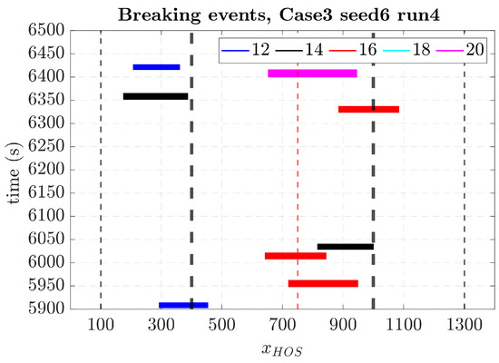
Figure 9.
Examples of wave breaking events identified using the Tian–Barthelemy breaking model for HOS-NWT waves. Each box represents space and time where and when the breaking events occur, and the color of the box corresponds to its wave crest height (). The thin black vertical lines represent the boundary of the CFD zone, whereas the thick black vertical dotted lines are the boundary between the pure CFD computational zone and the relaxation zone. The red vertical line is the reference position.
Figure 10 presents a comparison of the wave signal from the ECN experiment, the HOS-NWT simulation, and the OpenFOAM (foamStar) simulation of the test case Case3 Seed6. As in Figure 6, the wave time series, the time shift, and the correlations were compared using the HOS-NWT wave as a reference.
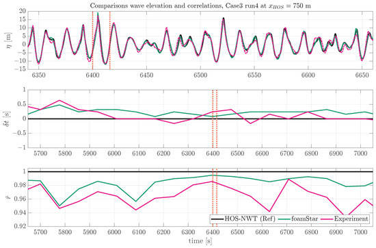
Figure 10.
Comparison of the wave elevation time series from the experiment foamStar and HOS-NWT at m Case3 Seed6. The red vertical lines represent the wave breaking events.
In general, the wave signals from both foamStar and the experimental data demonstrated good agreement with the HOS-NWT results. Specifically, foamStar exhibited a larger correlation, while the experimental data showed a smaller time shift. During this event, both the foamStar and the experimental waves showed good agreement. However, after the wave breaking event, around 6400 s, a decrease in correlation was observed in the experimental waves. This result implies that the Tian–Barthelemy wave breaking model effectively replicates the dissipation of waves during the wave breaking event. However, the memory effect of the wave breaking event shown in the experiment was not fully reproduced in the HOS-NWT and foamStar simulations.
Another deterministic analysis was conducted that mainly aimed to compare the difference in the spatial distribution of the wave elevation during the wave breaking events. The spatial distribution of the wave elevation from the HOS-NWT, foamStar, and point measurement from the experiment were compared.
In Figure 11, the five plots present the spatial distributions of the wave elevation of the wave breaking event measured within the time interval of [5940 s, 5980 s] and the space range of , m. The vertical dotted lines are the boundaries between the pure computational zone and the relaxation zones in the foamStar simulation. The results of the CFD simulation were obtained from three different mesh refinements, which are listed in Table 6. Before the wave broke, the CFD waves globally followed the spatial distribution of HOS-NWT. When the wave breaking event occurred, the CFD waves deviated from HOS-NWT and their values were closer to the experimental measurements. This result was expected since the wave breaking model implemented in the HOS-NWT did not represent the exact physical process during the breaking phase. It was designed to be representative of the real physics in terms of postbreaking properties (energy dissipation and redistribution). This was validated in the observation that, after breaking, the waves quickly recovered the excellent agreement between the HOS-NWT, CFD-NWT, and EWT. Also, after the wave breaking event, the CFD results exhibited different patterns of local wiggling, depending on the mesh refinement level. This implies that the CFD mesh refinements used in the present study are sufficient to reproduce the wave breaking event.
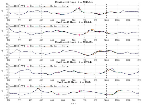
Figure 11.
Comparison of the wave profile from the HOS-NWT solver and foamStar solver with three resolutions during the wave breaking event of Case3 Seed6 Run4.
7.3. Stochastic Analysis
A stochastic analysis on the irregular waves was performed to estimate statistical properties and check the quality of the generated waves. The analysis was carried out using 10 realizations of waves measured at the target location. Each realization of a wave corresponded to approximately 3 h of measurements at full-scale.
7.3.1. Spectral Analysis
For spectral analysis, the averaged wave spectrum of 10 realizations was calculated and compared. The following analysis compares four different wave spectra, which are the target wave spectrum and the averaged wave spectrum obtained from the HOS-NWT, foamStar, and experiment. Figure 12 compares the mean wave spectra of Case1 and Case3 with the target spectrum. The x-axis is normalized to its peak wave frequency, and the y-axis is normalized to its significant wave height and peak period. The mean wave spectrum is defined as the average of all wave spectra from the 10 three-hour realizations. The following analysis compares four different wave spectra, which are the target wave spectrum and the averaged wave spectrum obtained from the HOS-NWT, foamStar, and experiment. Since the HOS-NWT waves were already corrected to the target spectrum, the HOS-NWT spectrum showed very good agreement. The foamStar results generally showed slightly underestimated results, and the experiment showed small oscillations around the target, depending on the wave frequency.
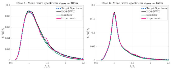
Figure 12.
Comparison of the irregular wave spectrum from the HOS-NWT, experiment, and foamStar for Case1 and Case3 at the target location m.
Figure 13 presents a quantitative comparison of the mean wave spectra by assessing the difference ratio between the wave spectra. The measured wave spectra are compared with the target spectrum on the left graph and also with the HOS-NWT spectrum on the right graph of Figure 13. A comparison with the HOS-NWT wave spectrum was considered important since the HOS-NWT was the input of the experiment and the CFD simulation. In this graph, the black dotted lines denote the bounds of the target criterion region, while the red dotted lines indicate the target frequency range of .
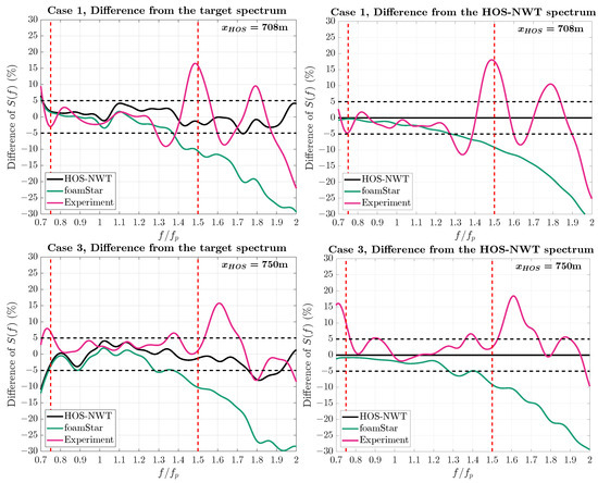
Figure 13.
Comparison of the irregular wave spectrum from the HOS-NWT, experiment, and foamStar for Case1 and Case3 at the target positions.
When the difference ratio of the wave spectrum from the target spectrum was compared, only the HOS-NWT spectrum satisfied the criterion in the target frequency range. On the other hand, comparing the experiment and the foamStar wave spectra using the HOS-NWT wave spectrum as a basis, neither of the two wave spectra satisfied the criterion in the target frequency range. The experimental result for both Case1 and Case3 generally aligned well with the HOS-NWT, while a larger discrepancy wave was measured for the high-frequency components. Looking at the variation in the wave spectrum in Figure 7, it suggests that the variation in the high-frequency components was related to the transverse effects in the wave basin. The foamStar simulation result generally showed a smaller wave spectrum than the HOS-NWT, and the wave spectrum gradually decreased as the wave frequency increased. Considering that the damping of a regular wave was highly related to the mesh resolution per wavelength, the underestimation of the spectrum, along with the frequency, was presumably due to the insufficient mesh resolution. The difference ratio of Case3 showed a more oscillatory reduction along the frequency than that of Case1.
Table 7 summarizes the wave parameters obtained at the target locations for both Case1 and Case3. It presents the significant wave height (), the wave peak period (, maximum of spectrum), and the true wave peak period () defined in Equation (4). The ITTC recommendation for wave modeling [13] proposed a tolerance of on both the significant wave height and the peak period. For both sea states, the significant wave heights and the wave peak periods of all wave spectra remained within the range .
Table 7.
Significant wave height, peak periods, and maximum difference ratio from the HOS-NWT spectrum of the irregular waves measured at m for Case1 and m for Case3.
In summary, the wave spectra of the foamStar simulations and the experiment generally showed good agreement with the HOS wave spectrum, while they did not satisfy the criterion in the entire target frequency range. Also, the wave parameters satisfied the ITTC recommendation.
7.3.2. Wave Crest Height Distribution
The PDSR (single realization) and PDER (ensemble realization) of the wave crest height were compared with the reference distributions. Note that the previous study of Canard et al. [30] showed that, depending on the target location from the wavemaker, even if the spectrum was qualified, the PDER curve of wave crest height could be significantly different. However, in this study, the target location from the wavemaker was only two and three wavelengths, and the evolution of the wave statistic properties along the domain was not expected to be significant. Figure 14 compares the probability of exceedance (POE) of the wave crest height measured at the target locations. The upper graphs show PDSR markers for Case1 and Case3, while the lower graphs show the PDER curves. Each PDSR marker presents a measured wave crest height. The y-axis of the graph presents the POE of the wave crest height, and the x-axis of the graph presents the normalized wave crest height. Note that the wave crest is normalized by the measured significant wave height tabulated in Table 7.
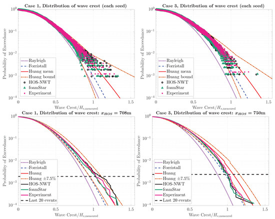
Figure 14.
Probability distribution of wave crests height at the target locations. The upper plots show the probability distribution of single realizations and the lower plots show the probability distribution of wave crest for an ensemble of realizations.
The PDSR markers of the experiments and numerical simulations were compared with a Rayleigh distribution, the Forristall distribution [28], and 99% of the upper and lower bounds of the wave crest distribution built by Huang and Zhang [25]. For Case1, the PDSR markers of the experiment, HOS-NWT, and foamStar mostly fell between the 99% lower and upper bounds of Huang’s distribution. Moreover, a few smaller wave crest heights of foamStar and larger wave crest heights of the experiment and HOS-NWT were captured. In the case of Case3, relatively smaller PDSR markers were captured compared to the Huang mean distribution.
The PDER curves were compared with the Huang ensemble distribution and the Forristall distribution. Additional bounds of the Huang ensemble distribution were also used to estimate the difference. The horizontal dotted line represents the probability of the last 20 events of the HOS-NWT simulation. In the PEDR analysis, the results under this dotted line are considered unreliable due to the lack of wave crest height data.
For Case1, overall, the three curves were in good agreement within the range of statistical convergence. Small discrepancies were observed forfoamStar, which predicted slightly underpredicted values. This might be related to the lower energy in the high-frequency range of the spectrum. Then, these curves compared quite well with the Huang PDER curve. For Case3, all three curves agreed well, excluding the last 20 events. This demonstrates that the wave breaking model in the HOS-NWT was able to correctly model the wave breaking observed in the CFD-NWT and the experiment. All three measured PDERs were underestimated compared to the Huang ensemble distribution.
8. Conclusions
The main objective of this paper was to propose and validate a wave generation and qualification procedure for irregular wave experiments and an OpenFOAM CFD simulation based on the HOS-NWT method. A wave generation and calibration procedure based on the HOS-NWT solver is proposed, and each part of the workflow is described. The details of the HOS-NWT wave solver are presented, and the setup of the wave basin experiment is outlined. Then, the numerical setup of the OpenFOAM simulation is introduced.
The proposed irregular wave generation process was tested for two long-crested irregular wave conditions: Case1 and Case3. One representing mild wave conditions and the other including frequent wave breaking events. For each wave condition, 10 three-hour realizations were performed to obtain the stochastic properties of the irregular waves. Finally, comparisons of the HOS-NWT, OpenFOAM (foamStar), and experiment were performed. Both deterministic and stochastic analyses were performed to assess the quality of the irregular waves, and the wave qualification criteria proposed for the stochastic analysis were applied. Finally, from the analysis, the following remarks can be made:
- Using the OpenFOAM solver foamStar, a split simulation with multiple time intervals was performed. The simulation was compared with the full 3 h simulation. Considering that the difference between the two simulations almost disappeared within for Case3, it was found that the influence of splitting is minimal and the memory effect from the nonlinearity of irregular waves is small. This result confirms that the split simulation of irregular waves is applicable. However, regarding its application to the WSI simulation, further investigation is required;
- In the deterministic analysis, a specific wave breaking event was selected for examination, focusing on comparing its time-series and spatial-wave profiles. The difference between the HOS-NWT, OpenFOAM, and experimental wave was small until they reached the wave breaking limit. When the HOS-NWT and OpenFOAM wave profiles were compared, a clear phase difference was captured, whereas a comparable wave dissipation was measured due to wave breaking. This finding suggests that the Tian–Barthelemy wave breaking model integrated into the HOS-NWT solver effectively replicates wave dissipation during the wave breaking event, while it does not induce a phase change associated with wave breaking events. The resultant waves of OpenFOAM generally followed the HOS-NWT, but they deviated from the HOS-NWT when wave breaking occurred and matched well with those in the experiment. Therefore, the CFD simulation with the suggested workflow can be used to model wave breaking events;
- A stochastic analysis of the wave spectrum was performed, comparing the measured wave spectrum with the target wave spectrum and the HOS-NWT wave spectrum. The wave parameters satisfied the ITTC criterion. The wave spectra of the OpenFOAM simulation and the experiment generally agreed well with the HOS-NWT wave spectrum, but they did not stay within the region in the entire target frequency range. The resultant OpenFOAM wave spectrum showed an underestimated wave spectrum, especially for the high-frequency components, due to an insufficient mesh resolution;
- A stochastic analysis was performed on the probability distribution of wave crest height. The measured PDSR and PDER curves were compared with the reference distributions. For both sea states, the PDSR markers fell mostly between the bounds of Huang’s empirical formula. For both Case1 and Case3, the three curves generally agreed well, excluding the last 20 events. This validates that, for Case3, the wave breaking model in the HOS-NWT can correctly model the wave breaking observed in the CFD-NWT and the experiment. Small underpredictions of the wave crest height were observed for foamStar, which might be related to the lower energy in the high-frequency range of the spectrum. For Case1, the PDER curves compared quite well with the Huang ensemble distribution, while smaller PDER curves were observed for the wave breaking condition. This result confirms that the suggested procedure effectively reproduces wave stochastic properties in both CFD simulations and experiments.
With these remarks, this study confirms that the HOS-NWT-based nonlinear irregular wave calibration and generation procedure, including the wave breaking model, can effectively reproduce nonlinear waves for both experiments and CFD-NWT simulations, saving experimental and computational time in wave calibration. However, the wave spectra of the experiment and CFD-NWT did not stay within the region in the target frequency range. The variation in the wave spectra of the experiment is considered to be an unavoidable error due to the wave basin characteristics and experimental limitations. In the case of the CFD-NWT, further studies on the CFD mesh resolution for irregular wave simulations are required to explore an adequate numerical setup for certain sea states.
Author Contributions
Conceptualization, Y.J.K., M.C. and B.B.; methodology, Y.J.K. and M.C.; validation, Y.J.K. and M.C.; formal analysis, Y.J.K. and M.C.; investigation, Y.J.K. and M.C.; software, Y.-M.C. and G.D.; writing—original draft preparation, Y.J.K. and M.C.; writing—review and editing, Y.-M.C., B.B., G.D. and D.L.T.; visualization, Y.J.K. and M.C.; supervision, Y.-M.C., B.B., G.D. and D.L.T.; project administration, B.B., G.D. and D.L.T.; funding acquisition, Y.-M.C., B.B., G.D. and D.L.T. All authors have read and agreed to the published version of the manuscript.
Funding
This research received no external funding.
Institutional Review Board Statement
Not applicable.
Informed Consent Statement
Informed consent was obtained from all subjects involved in the study.
Data Availability Statement
Data are contained within the article.
Acknowledgments
This work was performed in the framework of the Chair Centrale Nantes—Bureau Veritas on the Hydrodynamics of Marine Structures and was supported by the WASANO project, funded by the French National Research Agency (ANR) as part of the “Investissements d’Avenir” Programme (ANR-16-IDEX-0007). We also acknowledge funding from the Joint Industry Project Reproducible Offshore CFD JIP [18]. This research was supported by Basic Science Research Program through the National Research Foundation of Korea (NRF) funded by the Ministry of Education (RS-2023-00243370).
Conflicts of Interest
The authors declare no conflicts of interest.
Abbreviations
| WSI | Wave–Structure Interaction |
| OpenFOAM | Open-source Field Operation And Manipulation |
| CFD | Computational Fluid Dynamics |
| EWT | Experimental Wave Tank |
| NWT | Numerical Wave Tank |
| HOS | High-Order Spectral |
| FVM | Finite Volume Method |
| JONSWAP | JOint North Sea WAve Project |
| PDSR | Probability Distribution of the wave crest heights from Single Realizations |
| PDER | Probability Distribution of the wave crest heights from Ensemble Realizations |
| VOF | Volume Of Fluid |
References
- ITTC. Recommended Procedures and Guidelines: 7.5-02-07-02.1 Seakeeping Experiment; ITTC Association: Zürich, Switzerland, 2021; Revision 07. [Google Scholar]
- Chuang, T.C.; Yang, W.H.; Yang, R.Y. Experimental and numerical study of a barge-type FOWT platform under wind and wave load. Ocean Eng. 2021, 230, 109015. [Google Scholar] [CrossRef]
- Mohapatra, S.C.; Islam, H.; Hallak, T.S.; Soares, C.G. Solitary Wave Interaction with a Floating Pontoon Based on Boussinesq Model and CFD-Based Simulations. J. Mar. Sci. Eng. 2022, 10, 1251. [Google Scholar] [CrossRef]
- Gao, J.l.; Lyu, J.; Wang, J.h.; Zhang, J.; Liu, Q.; Zang, J.; Zou, T. Study on Transient Gap Resonance with Consideration of the Motion of Floating Body. China Ocean Eng. 2022, 36, 994–1006. [Google Scholar] [CrossRef]
- Chawla, A.; Kirby, J.T. A source function method for generation of waves on currents in Boussinesq models. Appl. Ocean Res. 2000, 22, 75–83. [Google Scholar] [CrossRef]
- Gao, J.; Ma, X.; Dong, G.; Chen, H.; Liu, Q.; Zang, J. Investigation on the effects of Bragg reflection on harbor oscillations. Coast. Eng. 2021, 170, 103977. [Google Scholar] [CrossRef]
- Gao, J.; Shi, H.; Zang, J.; Liu, Y. Mechanism analysis on the mitigation of harbor resonance by periodic undulating topography. Ocean Eng. 2023, 281, 114923. [Google Scholar] [CrossRef]
- Wang, L.; Robertson, A.; Kim, J.; Jang, H.; Shen, Z.R.; Koop, A.; Bunnik, T.; Yu, K. Validation of CFD simulations of the moored DeepCwind offshore wind semisubmersible in irregular waves. Ocean Eng. 2022, 260, 112028. [Google Scholar] [CrossRef]
- Shemer, L.; Sergeeva, A.; Liberzon, D. Effect of the initial spectrum on the spatial evolution of statistics of unidirectional nonlinear random waves. J. Geophys. Res. Ocean. 2010, 115, C12039. [Google Scholar] [CrossRef]
- Latheef, M.; Swan, C. A laboratory study of wave crest statistics and the role of directional spreading. Proc. R. Soc. A Math. Phys. Eng. Sci. 2013, 469, 20120696. [Google Scholar] [CrossRef]
- Janssen, P.A. Nonlinear four-wave interactions and freak waves. J. Phys. Oceanogr. 2003, 33, 863–884. [Google Scholar] [CrossRef]
- Fedele, F.; Cherneva, Z.; Tayfun, M.A.; Guedes Soares, C. Nonlinear Schrödinger invariants wave statistics. Phys. Fluids 2010, 22, 1–9. [Google Scholar] [CrossRef]
- ITTC. Recommended Procedures and Guidelines: 7.5-02-07-01.2 Laboratory Modelling of Waves; ITTC Association: Zürich, Switzerland, 2021; Revision 01. [Google Scholar]
- West, B.J.; Brueckner, K.A.; Janda, R.S.; Milder, D.M.; Milton, R.L. A new numerical method for surface hydrodynamics. J. Geophys. Res. Ocean. 1987, 92, 11803–11824. [Google Scholar] [CrossRef]
- Dommermuth, D.G.; Yue, D.K. A high-order spectral method for the study of nonlinear gravity waves. J. Fluid Mech. 1987, 184, 267–288. [Google Scholar] [CrossRef]
- Ducrozet, G.; Bonnefoy, F.; Le Touzé, D.; Ferrant, P. A modified High-Order Spectral method for wavemaker modeling in a numerical wave tank. Eur. J. Mech. B/Fluids 2012, 34, 19–34. [Google Scholar] [CrossRef]
- Canard, M.; Ducrozet, G.; Bouscasse, B. Generation of 3-hr long-crested waves of extreme sea states with HOS-NWT solver. In Proceedings of the 39th International Conference on Ocean, Offshore and Arctic Engineering (OMAE 2020), Online, 3–7 August 2020. [Google Scholar]
- Fouques, S.; Croonenborghs, E.; Koop, A.; Lim, H.J.; Kim, J.; Zhao, B.; Canard, M.; Ducrozet, G.; Bouscasse, B.; Wang, W.; et al. Qualification Criteria for the Verification of Numerical Waves—Part 1: Potential-Based Numerical Wave Tank (PNWT). In Proceedings of the ASME 2021 40th International Conference on Ocean, Offshore, and Arctic Engineering, Virtual, 21–30 June 2021. [Google Scholar]
- Hasselmann, K.; Barnett, T.P.; Bouws, E.; Carlson, H.; Cartwright, D.E.; Eake, K.; Euring, J.A.; Gicnapp, A.; Hasselmann, D.E.; Kruseman, P.; et al. Measurements of wind-wave growth and swell decay during the joint North Sea wave project (JONSWAP). Ergnzungsh. Zur Dtsch. Hydrogr. Z. R. 1973, 8, 1–95. [Google Scholar]
- Serio, M.; Onorato, M.; Osborne, A.; Janssen, P. On the computation of the Benjamin-Feir Index. Nuovo Cim. Della Soc. Ital. Di Fis. C 2005, 28, 893–903. [Google Scholar] [CrossRef]
- Papadimitriou, S.; Sun, J.; Yu, P.S. Local correlation tracking in time series. In Proceedings of the Sixth International Conference on Data Mining (ICDM’06), Hong Kong, China, 18–22 December 2006; pp. 1–10. [Google Scholar] [CrossRef]
- Choi, Y.M.; Bouscasse, B.; Ducrozet, G.; Seng, S.; Ferrant, P.; Kim, E.S.; Kim, Y.J. An efficient methodology for the simulation of nonlinear irregular waves in computational fluid dynamics solvers based on the high order spectral method with an application with OpenFOAM. Int. J. Nav. Archit. Ocean Eng. 2023, 15, 100510. [Google Scholar] [CrossRef]
- Welch, P.D. The Use of Fast Fourier Transform for the Estimation of Power Spectra: A Method Based on Time Averaging Over Short, Modified Periodograms. IEEE Trans. Audio Electroacoust. 1967, 15, 70–73. [Google Scholar] [CrossRef]
- Young, I.R. The determination of confidence limits associated with estimates of the spectral peak frequency. Ocean Eng. 1995, 22, 669–686. [Google Scholar] [CrossRef]
- Huang, Z.; Zhang, Y. Semi-empirical single realization and ensemble crest distributions of long-crest nonlinear waves. In Proceedings of the ASME 2018 37th International Conference on Ocean, Offshore and Arctic Engineering, Madrid, Spain, 17–22 June 2018; Volume 1. [Google Scholar] [CrossRef]
- Brown, L.D.; Cai, T.T.; Das Gupta, A. Interval estimation for a binomial proportion. Stat. Sci. 2001, 16, 101–117. [Google Scholar] [CrossRef]
- Longuet-Higgins, M.S. On the Statistical Distribution of the Heights of Sea Waves. J. Mar. Res. 1952, 11, 245–266. [Google Scholar]
- Forristall, G.Z. Wave crest distributions: Observations and second-order theory. J. Phys. Oceanogr. 2000, 30, 1931–1943. [Google Scholar] [CrossRef]
- Onorato, M.; Osborne, A.R.; Serio, M.; Cavaleri, L.; Brandini, C.; Stansberg, C.T. Extreme waves, modulational instability and second order theory: Wave flume experiments on irregular waves. Eur. J. Mech. B/Fluids 2006, 25, 586–601. [Google Scholar] [CrossRef]
- Canard, M.; Ducrozet, G.; Bouscasse, B. Varying ocean wave statistics emerging from a single energy spectrum in an experimental wave tank. Ocean Eng. 2022, 246, 110375. [Google Scholar] [CrossRef]
- Tian, Z.; Perlin, M.; Choi, W. An eddy viscosity model for two-dimensional breaking waves and its validation with laboratory experiments. Phys. Fluids 2012, 24, 036601. [Google Scholar] [CrossRef]
- Barthelemy, X.; Banner, M.L.; Peirson, W.L.; Fedele, F.; Allis, M.; Dias, F. On a unified breaking onset threshold for gravity waves in deep and intermediate depth water. J. Fluid Mech. 2018, 841, 463–488. [Google Scholar] [CrossRef]
- Canard, M.; Ducrozet, G.; Bouscasse, B. Experimental reproduction of an extreme sea state in two wave tanks at various generation scales. In Proceedings of the OCEANS 2022—Chennai, Chennai, India, 21–24 February 2022. [Google Scholar]
- Jasak, H. Error Analysis and Estimation for the Finite Volume Method with Applications to Fluid Flows. Ph.D. Thesis, Imperial College of Science, Technology and Medicine, London, UK, 1996. [Google Scholar]
- Seng, S. Slamming and Whipping Analysis of Ships. Ph.D. Thesis, Technical University of Denmark, Kongens Lyngby, Denmark, 2012. [Google Scholar]
- Larsen, B.E.; Fuhrman, D.R. On the over-production of turbulence beneath surface waves in Reynolds-averaged Navier-Stokes models. J. Fluid Mech. 2018, 853, 419–460. [Google Scholar] [CrossRef]
- Kim, Y.J.; Bouscasse, B.; Seng, S.; Le Touzé, D. Efficiency of diagonally implicit Runge-Kutta time integration schemes in incompressible two-phase flow simulations. Comput. Phys. Commun. 2022, 278, 108415. [Google Scholar] [CrossRef]
- Jacobsen, N.G. waves2Foam Manual; Technical Report August; Deltares: Delft, The Netherlands, 2017. [Google Scholar]
Disclaimer/Publisher’s Note: The statements, opinions and data contained in all publications are solely those of the individual author(s) and contributor(s) and not of MDPI and/or the editor(s). MDPI and/or the editor(s) disclaim responsibility for any injury to people or property resulting from any ideas, methods, instructions or products referred to in the content. |
© 2024 by the authors. Licensee MDPI, Basel, Switzerland. This article is an open access article distributed under the terms and conditions of the Creative Commons Attribution (CC BY) license (https://creativecommons.org/licenses/by/4.0/).