Research on Fault Diagnosis Method for Marine Diesel Engines Based on Multi-Scale Attention Mechanism Transformer

Abstract

In modern intelligent shipping, ensuring the stable and reliable technical condition of marine diesel engines is critical for safe and efficient vessel operations. Conventional fault diagnosis approaches and many existing Transformer-based methods often focus on single-scale features, potentially overlooking subtle fault indicators and reducing diagnostic accuracy under complex working conditions. To address these limitations, this paper proposes a Multi-Scale Attention Transformer (MSAT) model that integrates both high- and low-resolution attention mechanisms. This multi-scale strategy enhances the extraction of detailed and coarse-grained features, improving the model’s capacity to detect and characterize complex diesel engine faults. Additionally, an optimized Nadam optimizer is employed to refine convergence speed and accuracy, surpassing the Adam-based baseline by 0.71%. Rigorous testing on a publicly available diesel engine fault dataset demonstrates that the MSAT model achieves a diagnostic accuracy of 99.86% at a 60 dB signal-to-noise ratio (SNR), outperforming established models such as GRU and LSTM by more than 1%. Even under severe noise interference (0 dB SNR), the model maintains a high accuracy of 96.86%, highlighting its robustness and suitability for real-time monitoring in challenging marine environments. By quantitatively validating these improvements in diagnostic accuracy and noise resistance, this work offers a novel and effective solution for predictive maintenance and operational condition assessment of marine diesel engines, contributing to the reliability and safety of intelligent shipping systems.

1. Introduction

As the intelligent and complex development of marine and offshore engineering equipment advances, the health monitoring and fault diagnosis of critical electromechanical systems (such as marine diesel engines) have become increasingly important in ensuring safe and efficient ship operations [1,2]. Marine diesel engines, which operate primarily at low to medium speeds (~200–1500 RPM), are a cornerstone of modern marine propulsion systems, offering substantial thermal efficiency and power output for ships and offshore platforms. Although alternative fuels have been explored for enhancing engine performance, these traditional engines still provide irreplaceable value in terms of long service life and reliable performance in marine transportation and engineering [3]. However, the complex structure of diesel engines, combined with continuous operation in high-temperature and high-pressure environments, makes them highly susceptible to faults, posing risks to navigational safety while increasing maintenance costs and downtime [4,5]. While methods such as Weibull analysis have long been used for fault prediction and failure analysis, there is still a growing need for more efficient and precise real-time monitoring and fault diagnosis techniques for diesel engines. These advanced methods are essential for enhancing navigational safety and reducing economic losses by providing timely and accurate fault detection under dynamic operational conditions [6].

Traditional fault diagnosis methods for marine diesel engines include oil analysis, parameter detection, instantaneous speed monitoring, and vibration analysis, typically relying on specialized sensors and experienced engineers to manually assess equipment conditions [7,8,9,10]. While these methods can identify abnormal equipment conditions to some extent, their diagnostic accuracy and real-time performance are limited. They are susceptible to subjective factors and are not well suited to the complex and variable operational conditions of ships. For instance, traditional monitoring techniques mainly focus on abnormal parameters within the diesel engine, such as oil and water temperature, which may only exhibit noticeable changes once the fault has worsened to a certain degree, thus hindering the timely detection of early fault symptoms [11]. Consequently, there is an urgent need to develop intelligent, high-precision diagnostic methods that can adapt to complex operating conditions and enhance real-time performance [12].

Meanwhile, artificial intelligence (AI) optimization techniques, including genetic algorithms (GA), have been extensively studied for enhancing the performance of marine engines and supporting fault diagnosis. For instance, reference [13] utilized a genetic algorithm to optimize the valve timing and fuel injection parameters of low-speed marine diesel engines, leading to improvements in engine torque and fuel efficiency, as well as reductions in NO_x emissions. Furthermore, by employing multi-objective optimization, the study identified the optimal parameter configurations for different objectives, significantly enhancing engine performance and thermal conditions. Additionally, reference [14] introduced a novel machine learning approach—deep autoencoding support vector regression (DASVR)—for the online optimization and fault diagnosis of marine diesel engines. This algorithm combines the non-linear feature extraction capabilities of artificial neural networks (ANN) with the adaptability of support vector regression (SVR) to low-dimensional input spaces. Experimental results demonstrated that DASVR-based predictive models outperformed conventional ANN and SVR models, achieving maximum prediction errors of less than 3.8% across five key output variables under various operating conditions. The DASVR models also demonstrated superior real-time capability, meeting the real-time requirements for engine speeds below 3000 rpm. This approach provides an effective tool for the optimization of marine diesel engine performance and fault diagnosis, offering significant improvements in both prediction accuracy and computational efficiency.

Current research in marine diesel engine state monitoring and fault prediction can be categorized into three main approaches: knowledge-based, model-based, and data-driven methods. Knowledge-based methods rely on expert experience and predefined rules to identify faults. For example, Petar Vrvilo et al. [15] used virtual models to diagnose real-time data of marine diesel engines by comparing deviations with factory reference values, and utilized expert rules and heuristic methods for fault prediction, verifying the system’s effectiveness in reducing unplanned downtime and improving diagnostic accuracy. Haosheng Shen et al. [16] constructed a 0D/1D simulation model of a low-speed dual-fuel engine for marine applications to analyze the impact of turbocharger performance decay on engine performance and emissions, revealing significant influences of turbocharger decay on engine efficiency and emission characteristics under different combustion modes. Additionally, Nerveen M.T. Fahmy et al. [17] developed a fuzzy logic-based expert system that uses intelligent monitoring and supervisory systems for real-time fault detection and diagnosis, facilitating intelligent decision-making and optimized control of engine operating conditions to reduce fuel consumption and emissions. Knowledge-based methods are advantageous in fault identification under conditions of limited data, as they can leverage expert rules, providing strong interpretability; however, they are heavily reliant on expert knowledge and lack scalability. Model-based approaches simulate system behavior to achieve accurate diagnosis and prediction under complex conditions with a high degree of automation, but they require high-quality data and are costly to build and maintain.

In contrast, data-driven methods excel in adapting to complex environments and achieving self-optimization, particularly suitable for monitoring in challenging marine conditions. These methods leverage extensive historical data, making them highly capable of handling diverse fault modes and enhancing prediction accuracy. However, traditional two-step diagnostic methods typically consist of feature extraction and classification. In feature extraction, time-domain, frequency-domain, and time-frequency analysis methods are commonly employed to process raw data and extract characteristic information associated with system faults. Popular methods include Fourier transform [18], wavelet transform [19], and empirical mode decomposition [20]. During feature classification, techniques such as support vector machines (SVM) [21], artificial neural networks (ANN) [22], and decision trees [23] are commonly used to classify the extracted features. These approaches often require manual feature selection and typically involve single features with substantial redundant information.

To address the limitations of traditional methods, Hinton et al. proposed the theory of deep learning in 2006 [24], offering a breakthrough approach through neural networks with multiple hidden layers that automatically extract increasingly complex features from data. With the development of GPUs, computational power has significantly increased, fostering the successful application of deep learning across fields such as computer vision [25], autonomous driving [26], and natural language processing [27]. In the domain of fault diagnosis, the introduction of deep learning has brought enhanced diagnostic capabilities, especially for capturing nonlinear and complex pattern features. Deep learning methods eliminate the need for manual feature extraction by automatically extracting hierarchical features and performing classification diagnosis, and they support parallel processing of multiple signals. For example, a diesel engine operating condition recognition method based on a one-dimensional convolutional long short-term memory (LSTM) network achieved an accuracy of 99.08% [28]. In another study, an attention mechanism was introduced to CNNs, enhancing recognition accuracy by emphasizing key information [29]. Additionally, a Transformer model with stacked self-attention mechanisms was utilized to represent text [30]. Although these methods have achieved promising results, they still face limitations in handling complex fault signals, such as insufficient consideration of multi-scale features in signals. Therefore, effectively capturing multi-scale characteristics of fault signals to further enhance diagnostic accuracy remains an area that warrants in-depth exploration.

In the field of deep learning, some studies have attempted to combine multi-scale concepts with existing models to improve fault diagnosis outcomes. For example, [31] proposed a multi-scale convolutional neural network (MSCNN)-based network traffic monitoring method, which introduced convolutional kernels of different scales within the model, effectively extracting various scale features in network traffic data and substantially improving detection accuracy of network attacks and abnormal behaviors. Similarly, [32] employed an LSTM network for marine diesel engine fault prediction, achieving high-precision predictions of equipment remaining useful life (RUL) by learning the temporal dependencies in sensor data. This method leveraged LSTM networks to capture long-distance dependencies, demonstrating good generalization performance under different load conditions. However, these methods primarily rely on convolution operations or LSTM’s time-series modeling to achieve multi-scale feature extraction and temporal information capture, with some limitations remaining. While convolution operations can capture local and various scale features, they lack flexible global dependency modeling capabilities. Conversely, LSTMs excel at capturing long-range temporal dependencies but face certain limitations in multi-scale feature extraction. Thus, combining multi-scale feature extraction mechanisms with Transformer models, leveraging attention mechanisms to model both long- and short-distance dependencies, is an important research direction. This approach not only captures multi-scale features in signals but also comprehensively models long-range dependencies between different features, thereby enhancing diagnostic accuracy and robustness.

In response, we propose a Multi-Scale Attention Transformer (MSAT) fault diagnosis model. The primary quantifiable objective of this study is to accurately classify and identify specific diesel engine fault conditions—such as reduced intake manifold pressure or decreased cylinder compression ratio—based on directly measured engine parameters (e.g., cylinder pressure signals) under varying noise levels. Specifically, we aim to achieve at least 99% classification accuracy at a high signal-to-noise ratio (SNR = 60 dB) and maintain at least 95% accuracy even under severe noise interference (SNR = 0 dB). These measurable targets allow for a clear and objective evaluation of the model’s ability to detect abnormal engine states from raw sensor data.

To achieve this, the MSAT model introduces both low-resolution and high-resolution attention heads within the Transformer structure, enabling it to capture multi-scale feature representations directly from engine pressure signals and other key parameters. By applying attention mechanisms across multiple resolutions and effectively integrating information from different scales, the model significantly enhances its capability to detect subtle fault characteristics embedded in the engine parameter variations. Additionally, our model incorporates an optimized Nadam optimizer, which, compared to Adam, improves classification accuracy by 0.71%.

Experimental validation on public diesel engine fault datasets demonstrates that the MSAT model meets these defined quantitative goals, consistently maintaining high diagnostic accuracy across varying SNR conditions. This exceptional anti-interference performance underscores the model’s robustness and its practical utility for real-time monitoring and early fault detection in complex marine engine operating environments.

2. Materials

The components of Transformer include input embedding, position encoding, encoder, decoder, output embedding, layer normalization, and residual concatenation. Since its emergence, Transformer has made outstanding contributions in many fields such as image classification and generation in computer vision, time series prediction in finance and weather forecasting, text generation in natural language processing, and machine translation. The Transformer model improves the computational efficiency of the entire model due to its parallel processing capability, modeling advantages for long-distance dependencies, interpretability, flexibility, and high performance.

The overall architecture of the Transformer is illustrated in the Figure 1.

Because in classification tasks, the class task only needs to map the input to a single category without generating a sequence, the encoder can extract features to complete classification, while the decoder is complex and unnecessary, and may also increase computational costs. Transformer decoders are usually not used.

The structure of Transformer’s encoder consists of the following parts:

(1)

Multi-head self-attention mechanism: This serves as an enhancement of the self-attention mechanism. The multi-head self-attention mechanism allows the model to perform parallel computation on different “attention heads” and extract information from different subspaces. This is the core component of the encoder. The following is an introduction to its formula:

$$\mathrm{Attention}(Q,K,V)=soft\max ({\displaystyle \frac{Q\cdot K^T}{\sqrt{d_k}}})\cdot V$$

(1)

where Q, K, and V are the query matrix, key matrix, and value matrix, respectively. Q·K^T represents the attention level in the Transformer, and ${\displaystyle \frac{1}{\sqrt{d_k}}}$ is used for normalization processing to improve training effectiveness.

(2)

Feedforward Neural Network: This is located after each encoder and decoder layer. A feedforward neural network is a fully connected architecture that comprises two linear transformations followed by a nonlinear activation function. These three parts are performed sequentially, with activation functions typically inserted between two linear transformations. Its function is to perform fully connected transformation on the vector after position encoding or decoding, enhancing the representation of position information and feature extraction. By expanding the depth and width of the feedforward neural network, the Transformer model enhances its ability to capture the global relationships within the input sequence. Its formula can be expressed as follows:

$$FFN(X)=W_2\sigma (W_{1}X)$$

(2)

Among them, W₁ and W₂ represent the parameter matrices of two linear transformations and represent nonlinear activation functions, such as GELU.

Furthermore, the Transformer incorporates a residual connection at each sub-layer of both the encoder and decoder. This approach helps to mitigate the issue of vanishing gradients and enhances the flow of feature information, leading to improved model performance. Its formulation is

$$sublayerconnect(X)=X+sublayer(X)$$

(3)

After residual connection, layer normalization is used to process the input data and convert them into a standard normal distribution. The calculation formula can be expressed as follows:

$$u_i={\displaystyle \frac{1}{m}}{\displaystyle {\sum }_{j=1}^m{x}_{ij}}$$

(4)

$${\sigma }^2={\displaystyle \frac{1}{m}}{\displaystyle {\sum }_{j=1}^m(x_{ij}}-u_i{)}^2$$

(5)

$$layerNorm(x_i)=\alpha {\displaystyle \frac{x_{ij}-u_i}{\sqrt{{{\sigma }_i}^2+\epsilon }}}+\beta$$

(6)

where $u_i$ represents the mean of the i-th row in the input matrix, ${\sigma }_i$ represents the standard deviation of the i-th row, $\epsilon$ is used to avoid the denominator being zero, and $\alpha$ and $\beta$ are the learning parameters of the normalization layer.

3. Method

3.1. Proposed Model

The on-site working conditions are complex, and the working conditions of diesel engines are varied. The collected signals are often interfered with by high-frequency components and strong background noise, and the fault characteristics are easily masked. Therefore, some conventional machine learning and deep learning approaches fail to capture enough features from the raw signal to comprehensively characterize the state of the diesel engine. In order to better capture the fault features in the original signal, an improved multi-scale attention mechanism Transformer fault diagnosis method is proposed, which incorporates the multi-scale attention mechanism into the Transformer architecture and provides a more effective method to capture the multi-level features of the data by calculating attention weights at different scales. The model architecture is illustrated in Figure 2.

The model is mainly divided into three parts: encoder, multi-scale attention mechanism, and classification layer optimizer improvement. The encoder part replaces multi-head attention with multi-scale attention heads: (1) Low-resolution attention heads can use smaller feature dimensions, which allows the model to process input data at a rougher level and reduce computational complexity; and (2) High-resolution attention heads utilize complete feature dimensions. This allows the model to capture detailed characteristics of input data at a finer level. The multi-scale attention mechanism incorporates a one-dimensional average pooling operation on the original Transformer network architecture to reduce the temporal resolution of input data. Specifically, it simplifies input data by reducing the length of sequences while preserving important information as much as possible. This operation helps reduce computational complexity and allows the model to process input data at a rougher level. After being processed by a multi-scale attention mechanism, the original multi-head attention has been replaced by adding low-resolution attention heads and high-resolution attention heads, which can reduce the temporal resolution of the input data after passing through a one-dimensional average pooling layer, and allow two different resolution attention mechanisms to be applied later: (1) High-resolution attention mechanism: This part of the operation targets the original input data (high-resolution data), helping the model capture finer grained information and local features; and (2) Low-resolution attention mechanism: This part is applied to low-resolution data that have been average-pooled. Low-resolution views allow the model to capture a wider range of contextual information as it is not affected by high-frequency details. Finally, the final attention output is obtained by adding the high-resolution attention output and the upsampled low-resolution attention output. This approach can combine information from two scales, significantly improving the model’s overall understanding of input data and thus enhancing its performance.

3.2. Utilizing Improved Nadam for Data Optimization

Using the Nadam optimizer can achieve higher training accuracy, but in the early stages of training, there are severe oscillations in the iteration results, resulting in poor robustness. Therefore, this paper introduces a strategy of preheating the learning rate and gradually attenuating it.

Preheating and gradual decay of the learning rate are two commonly used strategies for adjusting the learning rate. By dynamically adjusting the learning rate, this approach improves model convergence, prevents instability during the initial phases of training, and mitigates the likelihood of overfitting in the later stages. Learning rate preheating is a process of gradually increasing the learning rate to a set initial value. When training neural networks, particularly during the initial stages, applying a high learning rate from the outset can result in excessive weight updates and potential model divergence. The preheating strategy starts from a small learning rate and gradually increases to a larger value to help the model stabilize in the early stages of training, improving its training stability and convergence speed. Gradual decay is a strategy of gradually reducing the learning rate during the learning process. As the training progresses, the model gradually approaches the optimal solution. If the learning rate remains elevated, it can lead to oscillations around the optimal solution, preventing the model from converging accurately. By gradually reducing the learning rate, the model can make more accurate weight adjustments when approaching the optimal solution, thereby improving the final performance and stability of the model. The formula for this strategy is as follows:

Take the reciprocal of the square root of the model dimension:

$$scale\_factor={\displaystyle \frac{1}{\sqrt{d_{model}}}}$$

(7)

where d_model represents the dimension of the model, and this factor is used to adjust the basic scale of the learning rate.

Reciprocal of square root of steps:

$$\arg 1={\displaystyle \frac{1}{\sqrt{t}}}$$

(8)

where t is the current number of training steps.

Learning rate adjustment based on preheating steps:

$$\arg 2=t\times T_{warm-up}^{-1.5}$$

(9)

where T_warm-up is the number of preheating steps, and this expression increases with the number of steps.

Take the minimum value between two adjustment values:

$$\min \_\arg =\min (\arg 1,\arg 2)$$

(10)

Ensure that the learning rate can gradually decline from a high value after the warm-up period ends. During the warm-up period, the learning rate is dominated by arg2, which gradually increases with the number of steps. After the warm-up period ends, arg1 (gradual decay factor) begins to dominate, causing the learning rate to decrease with increasing steps.

Final learning rate calculation:

$$\eta \left(t\right)=scale\_factor\times \min \_\arg$$

(11)

The learning rate rapidly increases to a large value during the warm-up period, and gradually decreases after the warm-up is over, which conforms to the general rule in deep learning that large-scale parameter models require a large learning rate in the initial stage to quickly approach the global optimum, and then a gradual decrease in the learning rate to fine-tune and avoid overfitting.

Nadam itself is an optimization algorithm that combines Adam and Nesterov acceleration gradients. It can dynamically adjust the learning rate by observing the magnitude and direction of gradients, enabling the model to converge faster during the training process. By introducing a weight decay factor, the model converges faster during the training process. Nadam incorporates the concept of adaptive moment estimation, adjusting the learning rate according to the historical gradient information related to the parameters to enhance the optimization process. In practical applications, Nadam optimization functions have demonstrated excellent performance in multiple deep learning tasks [33,34,35]. This has allowed Nadam to excel in a variety of machine learning tasks and complex deep learning architectures. The combination of Nadam and the strategy of learning rate preheating and gradual decay can combine Nadam’s adaptability with more detailed control achieved through learning rate scheduling.

3.3. Fault Diagnosis Method

Figure 3 illustrates the flowchart for the multi-scale attention mechanism Transformer used in fault diagnosis. The method can be summarized as follows:

(1)

Data preprocessing: Use a wavelet transform to transform each sample into rows, extract low-frequency coefficients from wavelet decomposition, perform singular value decomposition on the approximate coefficients obtained from wavelet transform, and extract feature vectors from the results of singular value decomposition, including statistical characteristics such as mean, variance, standard deviation, and skewness. Add class labels and shuffle the data, and normalize the features using normalization. Finally, the ratio of the training set to the testing set is 8:2.

(2)

Model training: Firstly, build a fault diagnosis model. Then, label encoding is used to convert the labels into one hot encoding, as the Transformer model expects the input format of a 3D tensor. Then, the training set is input into the model, and a multi-scale attention mechanism is used to extract multi-scale features and capture them. Finally, a cross entropy loss function is constructed, and the learning rate preheating and gradual decay strategy optimization algorithm is used for backpropagation. The model parameters are adjusted until the set number of iterations is reached, and the model parameters are saved.

(3)

Fault diagnosis: Import the test set data into a trained network model to obtain fault diagnosis results.

4. Results

This experiment adopts the TensorFlow framework in deep learning to achieve diesel engine fault classification and prediction. The experimental hardware environment is as follows: AMD Ryzen 7 5800H with Radeon Graphics CPU, manufactured by AMD in the Sunnyvale, CA, USA and produced in Taiwan, China, 16 GB RAM, NVIDIA GeForce RTX 3070 Laptop GPU, manufactured by NVIDIA in the Santa Clara, CA, USA and produced in Taiwan, China, Win11 operating system, Python 3.10.11

4.1. Description of the Experimental Platform

The experimental object is the operating dataset collected from the Acteon 6.12TCE series four-stroke cycle engines produced by MWM Diesel Engine Company, with specific parameters shown in

Table 1. Technical index of marine diesel engine.

Parameter Name	Parameter Value
Stroke Type	4 Strokes
Cylinders	6 in Line
Valve Control	On the Head Cylinder
Cylinder Valves	2 Valves
Diameter of the Cylinder	105 mm
Piston Stroke	137 mm
Connecting Rod Length	207 mm
Total Displacement	7118 L
Compression Ratio	16, 8:1
Inlet Valve Closing Angle	203°
Exhaust Valve Opening Angle	507°
Maximum Torque and Power	900 N.m/191 kW
Rotation (in Max. Torque)	1600 RPM
Ignition Order	1–5–3–6–2–4
Direction of Rotation	Counterclockwise (Viewed from Behind the Wheel)
Rail Pressure	350 a 1400 bar
Cooling Water Temperature	80–100 °C

[36].

4.2. Data Description

The experiment used the diesel engine characteristic fault feature dataset (3500 DEFault) from reference [37], which includes four scenarios: normal, intake manifold pressure reduction, reduced cylinder compression ratio, and reduced fuel injection into the cylinder, with a total sample size of 3500.

In the 3500 DE-Fault experiment, varying degrees of noise were introduced into the data, with signal-to-noise ratios of 0, 15, 30, and 60 dB, respectively. These noises are simulated by adding Gaussian white noise (AWGN) to the signal. In the basic configuration of the dataset, there are a total of 84 features included. These features include the maximum pressure curve values of six cylinders, the average pressure curve values of each cylinder, and the characteristics obtained through spectral analysis. The spectrum analysis section covers the frequency, amplitude, and phase of the first 24 harmonics, or the first 24 terms of frequency order.

4.3. Optimizer Selection

The optimizer used during model training plays a role in transmitting errors during training, and the choice of optimizer will affect the training results. Therefore, comparing the impact of five commonly used optimizers on training results, the findings are presented in Figure 4. In an environment with SNR = 15 dB, when the optimizer selects Nadam, its diagnostic accuracy reaches a maximum of 99.57%. And when the signal-to-noise ratio is 0 dB, it also has the highest accuracy of 96.86%. Therefore, Nadam was chosen as the optimizer for the model proposed in this article.

4.4. Number of Iterations

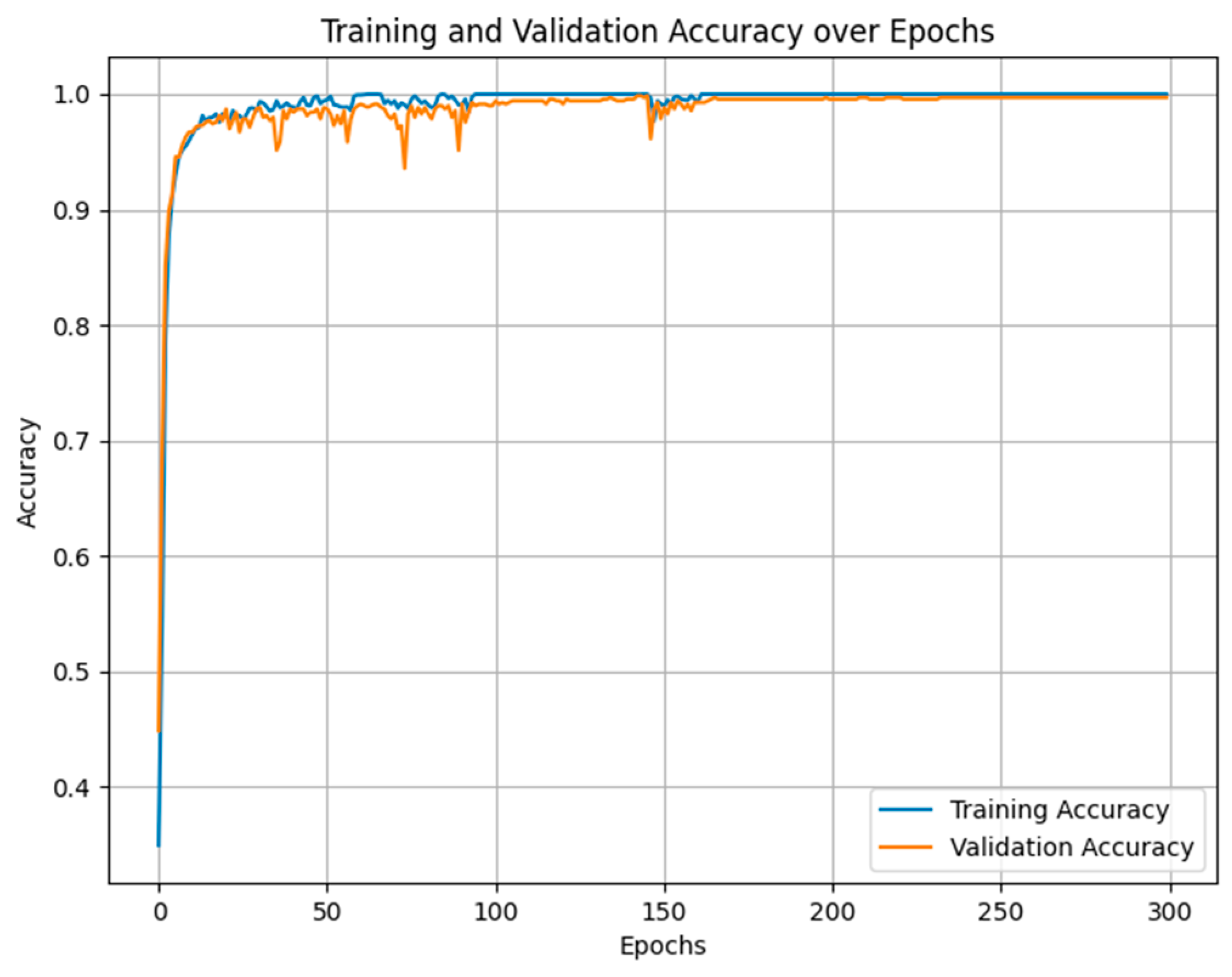
Figure 5 and Figure 6 illustrate the training accuracy and loss of the model using this method at an SNR of 15 dB. During the early stages of training, the Nadam optimizer causes both the training and validation accuracy to increase quickly, ultimately stabilizing around 1.0 after approximately 25 epochs. This outcome demonstrates that the model achieves nearly identical performance on both the training and validation datasets, reflecting an excellent learning effect. Throughout the entire training process, Nadam’s training curve and validation curve almost overlapped, and there was almost no significant overfitting phenomenon. The training and validation losses of the Nadam optimizer rapidly decreased and remained stable at a level close to 0, indicating that the model’s errors were well controlled throughout the entire training process. Although the validation loss fluctuates at certain moments, overall, it can quickly fall back to a lower level, reflecting the good robustness of the Nadam optimizer in the face of noise and uncertainty in the validation set data. Based on the above two charts, the Nadam optimizer has reached a good balance point around 50 epochs.

In the model training stage, the Nadam optimizer and the self-defined learning rate scheduler are used for backpropagation to update parameters. The core idea of the Nadam optimization algorithm is to combine the Adam optimizer with the Nesterov acceleration gradient, inheriting the advantages of Adam, and introducing the idea of NAG. The efficiency of optimization and the convergence of the model are further improved. In terms of the loss function of the model, the cross entropy loss function is used to calculate the output error. For hyperparameter settings in model training, the batch size is defined as 64, the number of iterations is established at 50 epochs, the random seed is chosen as 42, and the dropout value is set to 0.1. The learning rate is dynamically adjusted according to the training steps through a self-defined learning rate scheduler. The initial learning rate starts at a relatively high value and gradually decreases throughout training, allowing for quicker convergence towards the optimal solution in the early stages and more stable convergence later. This setup can better balance the speed and stability of learning.

4.5. Methods

To highlight the effectiveness of the proposed model, multi-scale attention mechanisms such as Transformer, LSTM, GRU, ELM, XGBOOST, etc. were tested and compared. Moreover, in practical applications, diesel engines usually operate in complex environments, and the collected fault signals are easily contaminated by noise. To evaluate the noise resistance capability of the diagnostic model discussed in this paper, Gaussian white noise at different signal-to-noise ratio levels was added to the dataset for classification training. Accuracy, Precision, Recall, and F1 Score were used to evaluate the generalization performance of the model at different signal-to-noise ratio levels.

Table 2. Diagnostic effect evaluation of different models in different noise environments.

Environment	Model	Accuracy (%)	Precision (%)	Recall (%)	F1-Score (%)
SNR = 0 dB	MSA-Transformer	96.86	96.99	96.86	96.90
	ELM	89.00	88.67	89.00	87.95
	GRU	93.86	94.27	93.86	94.00
	LSTM	95.86	96.24	95.86	95.97
	XGBOOST	86.00	86.97	86.00	85.61
SNR = 15 dB	MSA-Transformer	99.57	99.59	99.57	99.58
	ELM	94.71	94.77	94.71	94.60
	GRU	97.57	98.01	97.58	97.69
	LSTM	97.71	98.18	97.71	97.83
	XGBOOST	91.58	92.04	91.57	91.41
SNR = 30 dB	MSA-Transformer	99.85	99.85	99.85	99.85
	ELM	96.57	96.92	96.57	96.61
	GRU	98.14	98.46	98.14	98.22
	LSTM	98.29	98.56	98.29	98.35
	XGBOOST	91.29	91.65	91.29	91.18
SNR = 60 dB	MSA-Transformer	99.86	99.86	99.86	99.86
	ELM	97.00	97.37	97.00	97.06
	GRU	98.86	98.99	98.86	98.89
	LSTM	98.71	98.88	98.71	98.75
	XGBOOST	94.86	95.36	94.86	94.72

displays the test results for all models, in which the larger the values of each indicator, the better the classification performance of the model.

According to Table 2, when SNR = 60 dB, all four indicators of the proposed model are the highest, with an accuracy of 99.86%, surpassing the second place by 1%. As the noise intensity increases, the evaluation indicators of all models show a downward trend, but the proposed models are basically in a leading position. This indicates that the method proposed in this article, which utilizes global average pooling operations to apply multi-scale attention mechanisms of different resolutions, is effective in filtering out noise to a certain extent. It is worth noting that when the signal-to-noise ratio is 0 dB, the diagnostic accuracy of the proposed model is still as high as 96.86%, indicating that the proposed model has excellent anti-interference performance in noisy environments.

To provide a more intuitive view of the fault identification situation, Figure 7 and Figure 8 are the confusion matrices of this method. When SNR = 15 dB, only 3 out of 700 test samples were misclassified. Label 1 is normal, label 2 is a decrease in intake manifold pressure, label 3 is a decrease in cylinder compression ratio, and label 4 is a decrease in cylinder fuel quantity. The misclassified sample labels belong to the faulty cylinder compression ratio decrease. When SNR = 0 dB, the values on the diagonal are higher, indicating that most samples can be correctly classified, especially the two categories of “reduced cylinder compression ratio” and “reduced cylinder fuel quantity” (category 3 and category 4), which have very high accuracy, demonstrating the good robustness of the model under high noise conditions. The category of “reduced intake manifold pressure” also has a certain degree of accuracy in classification, but is more affected by noise. The model performs particularly well in category 3 (reduced cylinder compression ratio) and category 4 (reduced cylinder fuel quantity), which are usually crucial for engine fault diagnosis. The high accuracy of the model helps reduce missed detections and false positives.

To further understand the feature learning process of this method, t-SNE is employed to visualize the complete fault recognition process. Figure 9 shows the visualization of the original signal. Figure 10 shows a visualization of the MSAT model. After t-SNE dimensionality reduction, the distribution of various types of samples is relatively scattered, and the overlap between different categories is obvious. Especially for the categories of “normal” and “reduced cylinder compression ratio”, the sample distributions almost overlap, indicating poor separability of features between these two categories. After feature extraction using the MSAT model, different categories showed clearer distributions in t-SNE visualization: the distance between sample clusters of each category increased significantly, and the separation between different categories became more distinct. Especially in the categories of “reduced cylinder compression ratio” and “reduced cylinder fuel quantity”, the data point aggregation effect was good, demonstrating the feature extraction ability of this model under high noise conditions. The gap between the “normal” category and other fault categories is clearer, indicating that MSAT performs better in extracting distinguishing features between faults and normal states.

5. Discussion and Conclusions

The study presented a Multi-Scale Attention Transformer (MSAT) fault diagnosis model for marine diesel engines, effectively capturing multi-scale features through integrated high- and low-resolution attention heads. The model’s use of an enhanced Nadam optimizer further improved convergence speed and accuracy, facilitating precise fault classification under challenging conditions. Experimental results demonstrated that the MSAT model achieves high diagnostic accuracy—up to 99.86% at 60 dB SNR—and maintains robust performance (96.86% accuracy) even at 0 dB SNR. Compared to alternative methods such as LSTM, GRU, ELM, and XGBoost, MSAT consistently outperformed them across various metrics, confirming its superiority in handling complex fault characteristics and significant noise interference.

Compared to previous studies, this paper has made significant improvements in multi-scale feature extraction and model robustness. Zhenguo Ji et al. [38] proposed a deep learning-based hybrid neural network model (CNN BiLSTM Attention) for predicting and warning the exhaust temperature (EGT) of marine diesel engines. This model combines convolutional neural networks (CNN) to extract features from time series data, bidirectional long short-term memory networks (BiLSTM) for time series modeling, and attention mechanisms to improve prediction accuracy and robustness, outperforming traditional methods such as RNN and LSTM. Sun et al. [39] developed a CNN-LSTM model (CNN-LSTM-LLA) that integrates multi-layer attention mechanisms. By introducing multi-layer attention mechanisms into the CNN and LSTM modules, it further enhances the ability to extract features and capture temporal dependencies. However, these methods still struggle to comprehensively capture multi-scale feature information when dealing with fault signals in complex noisy environments, and the model’s anti-interference ability against noise is limited. The proposed MSAT model addresses these limitations by integrating high-resolution and low-resolution attention mechanisms and combining them with an optimized Nadam optimizer. This integration not only maintains a high accuracy of 96.86% under high noise conditions (0 dB SNR) but also demonstrates exceptional robustness and diagnostic precision across various noise levels. Consequently, the MSAT model significantly outperforms existing models such as GRU and LSTM to a certain extent, highlighting its enhanced capability in capturing multi-scale fault features and resisting noise interference.

Beyond its theoretical and experimental achievements, the MSAT model can be readily integrated into vessel engine monitoring and control systems. Real-time data from sensors—such as cylinder pressure, vibration, and exhaust gas composition—can be continuously analyzed by the MSAT model onboard. The system’s outputs can be translated into intuitive, quantifiable indicators (e.g., a “Fault Severity Index”), providing operators with actionable insights. Color-coded alerts and fault severity scores help the crew make informed maintenance decisions—planning inspections, adjusting operating conditions, or scheduling targeted repairs—before minor issues escalate into severe failures. Over time, accumulated diagnostic data assist in refining maintenance strategies, enhancing the reliability and long-term efficiency of marine diesel engines.

Looking ahead, the MSAT-based approach can be extended through selective integration with additional data sources and operational analytics. By correlating the model’s outputs with engine-specific maintenance logs and operational parameters, ship operators could better predict time-to-failure, optimize maintenance intervals, and potentially integrate the model’s recommendations into voyage planning decisions. Such enhancements could include fusing multiple sensor modalities to further improve accuracy and early fault detection, thereby evolving MSAT into a comprehensive decision-support tool. This future-oriented vision underscores the potential of the MSAT model as both a practical and scalable solution, meeting the evolving demands of intelligent shipping and contributing to safer, more efficient maritime operations.

Despite the demonstrated strengths, the MSAT model may encounter limitations when dealing with certain rare or previously unobserved fault patterns. For instance, if a fault type emerges only under highly specialized operating conditions—such as transient overloads combined with atypical fuel properties—and has limited representation in the training dataset, the model’s accuracy may decrease. In such scenarios, the multi-scale attention mechanism may struggle to isolate distinctive features due to insufficient exposure, and the optimized Nadam training strategy cannot fully compensate for the lack of representative samples. This leads to less confident classifications and occasional misdiagnoses. Understanding and addressing these limitations could involve data augmentation, incorporating domain adaptation techniques, or expanding the training dataset with a broader range of operating conditions and fault types. Such efforts would help ensure that the MSAT model evolves into a more universally robust solution, capable of handling not only common fault scenarios but also rare and complex failure modes encountered in diverse marine environments.

In summary, the MSAT model provides a robust and accurate solution for diesel engine fault diagnosis, demonstrating exceptional adaptability to challenging noise conditions and potential for real-time application. Future work will focus on enhancing the model’s adaptability through domain adaptation, exploring semi-supervised learning to reduce reliance on labeled data, and integrating predictive maintenance scheduling along with multi-sensor data fusion (e.g., thermal imaging, acoustic emission). By pursuing these directions, the MSAT model is poised to evolve into a more comprehensive decision-support system that keeps pace with advancements in marine engineering, ultimately contributing to safer, more efficient, and more intelligent ship operations.