Investigating Tidal Stream Turbine Array Performance Considering Effects of Number of Turbines, Array Layouts, and Yaw Angles

Abstract

The performance of a tidal stream turbine array can be affected by numerous factors. Investigating the connection between array power production and these factors will be helpful in improving the development of tidal stream energy. This study investigates the impact of array layout, turbine number, and yaw angles on turbine array performance using an open-source coastal ocean modelling system. The results show that the total power output of the turbine array rises with the number of turbines. Under realistic conditions, there are not many differences in power output between aligned and staggered turbine array configurations. By extending the distance between the turbines, the array power output can be improved in both layouts. It appears that considering each turbine’s yaw angle can improve array power generation, since the downstream turbines will greatly benefit from the steering wake of the upstream turbines. Furthermore, using a gradient-based optimization algorithm to simultaneously adjust the yaw angles and turbine positions will boost the turbine array’s efficiency more than just optimizing the turbine position alone.

1. Introduction

Greenhouse gasses and particulates generated during fossil fuel combustion can have serious environmental consequences and threaten human society’s long-term development [1]. As a result, many governments have agreed to pursue renewable and clean energy. Tidal stream energy, as one of the marine renewable energies, has received global interest due to its great predictability, energy density, and stability [2,3]. In China, the tidal stream energy can theoretically supply more than 8.2 GW [4]. However, unlike wind turbines, which can have diameters of more than 100 m, the diameter of a tidal stream turbine is restricted by sea depth. Since power output is proportional to the size of the spinning area, the tidal stream turbine’s limited diameter limits the power output of a single turbine. Thus, in order to obtain abundant energy extraction from the tidal steam, dozens or even hundreds of turbines are installed together to form a turbine array using the strategies similar to those utilized in wind turbines [5].

Vennell [6] demonstrated that in large tidal straits, turbines can exceed the Betz efficiency limit by filling the channel’s cross-section. However, as the number of turbines increases, interactions between turbines will unavoidably occur within the array, resulting in a drop in array power output [7]. As a result, numerous academics have focused their attention on the wake area and turbine layout. It is widely acknowledged that the wake region can extend to 40D (D is the diameter of the turbine) downstream, and the stream velocity can recover roughly 80% at a distance of 20D downstream [8,9].

Regarding the array layouts, the most popular and extensively researched options are aligned and staggered configurations. In a rectangular numerical channel, Divett et al. [10] examined the power output of four distinct configurations using 15 turbines arranged in 5 rows. They discovered that the aligned layout’s power production can be enhanced by the wider spacing. Nevertheless, the amount is still less than half of the array’s power output in the staggered arrangement. Draper and Nishino [11] used the linear momentum actuator disc theory to simulate turbines. They compared the power outputs from turbines arranged in different rows. They discovered that arranging turbines in a single row can produce more electricity than arranging them in two rows. The array’s power output for two rows in a staggered layout would be greater than the values in an aligned layout. Nash et al. [12] have also reported similar outcomes, using a multiscale nested model to predict the impact of layouts on array power outputs.

Intelligent optimization techniques have been utilized for investigating into the best turbine array layout due to the quick advancement of computing power. Combining the turbine wake model with the optimization algorithm is a popular method of optimization. For turbines with a small diameter to depth ratio, Lo Brutto et al. [13] presented an analytical wake model, which was then combined with a Particle Swarm optimization approach to optimize the turbine array layout [14].

Using the Discrete Particle Swarm optimization algorithm with Jensen wake model and elliptic distribution model, Wu et al. [15] enhanced the array layout. They found that the optimized array outperformed the staggered configuration by 6.19%. Wu et al. [16] included the levelized cost of energy model into the turbine array layout optimization and modified the optimization algorithm to the Quantum Discrete Particle Swarm algorithm. While the accuracy of the wake models is crucial to the dependability of these techniques, Funke et al. [17] presented an additional noteworthy method for optimizing layout. The turbine array layout optimization problem is determined to be a PDE-constrained optimization problem in their model, and they have developed an automated method for completing the optimization [18,19]. They used a gradient-based optimization methodology to optimize the array layout after coupling the shallow water equation with an adjoint method. The gradient was determined using the adjoint method. Numerous studies have employed this technique to examine the optimal array layout while taking into account the power production, array’s cost, and even environmental impact [20,21,22].

It should be noted that the effects of the yaw angle are disregarded in all of the aforementioned studies, by assuming that all turbines’ usual directions are in the best possible alignment with the flow. However, a tidal stream turbine’s thrust and power appear to change as well as the effective direction of the turbine race when it encounters misalignment in incident flow or yawed inflow, which causes the stream to become out of alignment with the turbine [23]. To understand the impacts of yaw angles, several experimental and numerical studies have been carried out [24,25,26,27]. It is determined that the turbine’s power production and rotor thrust decrease as the yaw angle increases.

The yaw angle of each turbine can also affect the array’s total power output. According to Modali [28], the downstream turbine’s power production increased when the upstream turbine was yawed. By taking into account the yaw angle, a staggered layout can be improved by up to 50% when compared to an aligned layout. When Badoe et al. [29] examined the performance of three array layouts with fourteen turbines, they discovered that even slight changes in the yaw angle had a significant impact on the overall power output.

As is evident, the impact of turbine count on array power production was mostly examined analytically or numerically in an ideal rectangular computing domain. Likewise, using the same approaches, the impact of aligned and staggered layouts on turbine array performance has been investigated. However, the impact of the number of turbines and array layouts on array performance in a realistic marine area has not been thoroughly studied. Furthermore, to the best of the author’s knowledge, there is no model that optimizes the tidal stream turbine array layout by taking into account the turbine yaw angle, which has a substantial impact on the array power output.

Therefore, in this study, the channel between Hulu Island and Putuoshan Island, which is situated in the Zhoushan Islands in the Chinese province of Zhejiang, has been chosen as the study area. To examine how the number of turbines and array layouts affect the performance of a tidal stream turbine array, a two-dimensional hydrodynamic model is developed based on the open-source coastal modelling framework, Thetis, which incorporates a gradient-based optimization technique and a yawed turbine model. The impact of yaw angles on array performance is examined by comparing the power outputs of arrays in aligned, staggered, and optimized layouts with and without taking the yaw angle into account.

2. Numerical Model

2.1. Governing Equations

In this study, as we focus on the two-dimensional simulation, the nonlinear shallow water equations are applied as the governing equations:

$$\begin{array}{c}{\displaystyle \frac{\partial \eta }{\partial t}}+\nabla \cdot \left(H\mathit{u}\right)=0\\ {\displaystyle \frac{\partial \mathit{u}}{\partial t}}+\mathit{u}\cdot \nabla \mathit{u}-v{\nabla }^2\mathit{u}+f{\mathit{u}}^{\perp }+g\nabla \eta =-{\displaystyle \frac{{\tau }_b}{\rho H}}-{\displaystyle \frac{c_t}{H}}\parallel \mathit{u}\parallel \mathit{u}\end{array}$$

(1)

where $\eta$ is the free surface displacement, $t$ is time, $H$ is the total water depth, $\mathit{u}$ is the depth-averaged velocity vector, $\nu$ is the kinematic viscosity, $f$ is the Coriolis frequency, and ${\tau }_b$ is the natural bottom shear stress. In the final term, $c_t$ is a dimensionless friction coefficient parameterizing the thrust force of the turbine, which is described in more detail in Equation (4) in Section 2.2.

2.2. Yawed Turbine Model

In the two-dimensional model of Thetis, the linear momentum actuator disc theory is applied to introduce turbines’ thrust and to quantify the energy extraction. The turbine is parameterized as regions of enhanced bottom friction, with a spatially varying non-dimensional bottom friction coefficient, $c_t$. Though this method has been widely used in many optimization studies [17,20,22], turbines are assumed to be always aligned with the flow. In this study, the turbine performance with a yaw angle, as shown in Figure 1, is considered.

By assuming that all flow forces are applied in the turbine normal direction and any transverse pressure gradients can be neglected, the thrust force and the power output forms for a yawed turbine has been derived [31], which show as follow:

$$F={\displaystyle \frac{1}{2}}{C_{t}A}_t\rho {\left(u_0\mathrm{c}\mathrm{o}\mathrm{s}\left(\theta \right)\right)}^2$$

(2)

$$P=F{u}_1={\displaystyle \frac{1}{4}}\left(1+\sqrt{1-C_t}\right)C_t\rho A_t{\left(u_0\mathrm{c}\mathrm{o}\mathrm{s}\left(\theta \right)\right)}^3$$

(3)

where $C_t$ is the thrust coefficient of the turbine, $A_t$ is the turbine cross-sectional area. $u_0$ is the upstream velocity, $u_1$ is the normal component of the ambient velocity through the turbine, and $\theta$ is the angle between the turbine normal direction and the direction of $u_0$.

For a single turbine, the relationship between dimensionless friction coefficient, $c_t$, and thrust coefficient, $C_t$, can be formed as:

$${\int }_A c_t=C_t{A}_t{\displaystyle \frac{4}{{\left(1+\sqrt{1-\frac{A_t}{{\widehat{A}}_t}{C}_t}\right)}^2}}$$

(4)

where $A$ is the actual area at which the thrust force is applied in the two-dimensional model. ${\widehat{A}}_t$ is the cross-section area in a three-dimensional model; its value can be approximated as the product of the turbine diameter and the water depth. A detailed derivation can be found in [30,31].

2.3. Optimization Model

A fully automated adjoint method [19] is equipped in Thetis, which enables the efficient computation of the gradient for a specific outcome from a model with respect to any input parameters. Thus, a gradient based optimization algorithm is applied to determine an optimal turbine array layout and the yaw angle for each turbine with a given number of turbines [18,32]. The optimization problem can be formulated as:

$$\begin{array}{cc}\hfill \underset{z,m}{max}\hfill & J(z,\mathbf{m})\hfill \\ \hfill \mathrm{s}\mathrm{u}\mathrm{b}\mathrm{j}\mathrm{e}\mathrm{c}\mathrm{t}\hspace{0.25em}\mathrm{t}\mathrm{o}\hfill & F(z,\mathbf{m})=0\hfill \\ & b_l\le \mathbf{m}\le b_{\mathrm{u}}\hfill \\ & g\left(\mathbf{m}\right)\le 0\hfill \end{array}$$

(5)

where $\mathit{J}(z,\mathit{m})$ is the function of interest,$F(z,\mathit{m})$ is a partial differential equations (PDE) operator containing the shallow water equations, such as those in Equation (1), $z=(\mathit{u}, \eta )$ is the tidal elevation and tidal velocity results of Equation (1), $b_l$ and $b_u$ are the bounds of the turbine deploying area, and $g\left(\mathit{m}\right)$ is the result of the allowed minimum distance minus the actual spacing between two turbines.

The gradient-based optimization is implemented with the L-BFGS-B quasi-Newton method. The overall procedure can be summarized as follows:

• Input the initial values of coordinates and yaw angles for each turbine, forming the parameter vector ${\mathit{m}}^{\mathit{i}}$.
• Solve the shallow water equation with the turbine-related information vector, ${\mathit{m}}^{\mathit{i}}$ and obtain the corresponding elevation field, ${\eta }^i$, and velocity field, ${\mathit{u}}^{\mathit{i}}$.
• Evaluate the functional of interest $\mathit{J}(z^i,{\mathit{m}}^{\mathit{i}})$ and compute the functional gradient $\mathrm{d}\mathit{J}/\mathrm{d}\mathit{m}$.
• Check if $\mathrm{d}\mathit{J}/\mathrm{d}\mathit{m}$ fulfils the optimization termination criteria. If so, stop and output the parameter vector, ${\mathit{m}}^{\mathit{i}}$, and the functional of interest, $\mathit{J}(z^i,{\mathit{m}}^{\mathit{i}})$. Otherwise, proceed to step 5.
• Improve parameter vector ${\mathit{m}}^{\mathit{i}}$ to ${\mathit{m}}^{\mathit{i}+1}$ using the quasi-Newton method and go to step 2 with ${\mathit{m}}^{\mathit{i}+1}$.

In this study, the termination criterion is that the maximum value of the projected gradient is less than 10⁻⁴.

2.4. Computational Domain and Its Meshing

Numerous investigations have confirmed that the channels surrounding Zhoushan Islands in Zhejiang Province, China, contain a significant amount of tidal stream energy. The first tidal stream engineering demonstration project is located in the channel between Hulu Island and Putuoshan Island, which is selected as the study region for this work. For simplicity, we refer to this channel as the HP channel.

As shown in Figure 2, the computational domain well covers the Hulu Island and Putuoshan Island, which varies from 122°16′ to 122°32′ at an east longitude and from 29°54′ to 30°09′ at a north latitude. The mesh size at the open sea boundary is 1500 m. To capture the land boundaries, the mesh size is set to 200 m. Given their potential to greatly impact the tidal stream in the HP channel, the mesh size is further fine-tuned to 50 m for the land borders of Hulu Island and Putuoshan Island. The Turbine Deploying Area (TDA), which is a rectangular space inside the HP channel that is 250 m long and 215 m wide, is where turbines are permitted to be installed. As noted in [17], turbine-resolving mesh resolution should be less than or equal to a quarter of the turbine diameter, which is constant at 20 m in this study. Thus, the mesh size inside the TDA is set to be 5 m. The final meshes have 20,648 vertices and 40,492 triangle elements.

Figure 3 shows the distribution of the water depth, which is an integrated outcome derived from the measured data. The HP channel’s typical water depth is around 40 m, making it appropriate for the installation of turbines with a 20 m diameter. Two stations, one for tidal elevation and one for tidal velocity, are situated within the HP channel, as illustrated in the dashed rectangle in Figure 3. The measurements are then used to validate the accuracy of simulation.

2.5. Solver Options and Boundary Conditions

For spatial discretization, both the tidal elevation and velocity fields are represented by piecewise linear discontinuous basis functions. The temporal discretization is performed using the backward Euler approach with a fixed time-step of five minutes. An 800-meter-wide sponge layer with higher viscosity and friction values is added to prevent erroneous reflections that could happen at an open boundary. At the open boundary, the viscosity and manning coefficients are set to be 1000 ${\mathrm{m}}^2{\mathrm{s}}^{-1}$ and 0.1 $\mathrm{s}/{\mathrm{m}}^{1/3}$, respectively. Within the sponger layer, they drop linearly to 0.01 ${\mathrm{m}}^2{\mathrm{s}}^{-1}$ and 0.02 $\mathrm{s}/{\mathrm{m}}^{1/3}$ and remain constant within the computational domain. It has been proven that adding a sponge layer can improve the stability of the model while having no impact on the HP channel simulation results [22,33,34].

A wetting and drying algorithm is used to capture the flow close to the land boundary. Two methods for creating the open boundary forcing are contrasted for the open boundary. For the ensuing research scenarios, the one that agrees better with the measured data from elevation and velocity stations is selected. Firstly, we select eight primary tidal constituents ($Q_1,$ $P_1,$ $O_1,$ $K_1,$ $M_2,$ $S_2,$ $N_2,$ $K_2$) from the TPXO9 Atlas [35] to form the force at the open boundary, which is named as Case OB1. Secondly, we create two field functions that each encompass the whole Zhoushan Island regions using the numerical elevation and velocity data from [33]. The elevation and velocity values at the open boundary are then integrated using two field functions. This case is called Case OB2.

2.6. Model Validation

2.6.1. Hydrodynamic Model Validation Data Sources

Through the tidal stream engineering demonstration project (GHME2015GC01), the measured tidal elevation and velocity data were acquired. The correctness of the tidal simulation procedure in this work is confirmed by measurements from a velocity station and an elevation station. The two stations’ locations are shown in Figure 3.

At station A, the measured tidal elevation data were collected from 2013.8.15 to 2013.8.25 with a temporal resolution of 1 h. At station B, the measured tidal velocity data are divided into a neap period (2013.8.16 10:00~2013.8.17 11:00), intermediate period (2013.8.19 14:00~2013.8.20 15:00), and spring period (2013.8.23 10:00~2013.8.24 11:00). The temporal resolution of the velocity measurement data is 10 min.

2.6.2. Turbine Model Validation Data Sources

The wake velocity distribution of a single turbine with a yaw angle ranging from 0~30$°$ is measured by Zhang et al. [26] in a recirculating flow flume designed and constructed at Hohai University, as shown in Figure 4. The flume is 50 m long, 5 m wide, and 0.7 m deep. The diameter of the turbine is 0.3 m. The water depth is fixed at 0.5 m, with a constant inflow velocity at 0.33 m/s, equating to a Froude number of 0.15. This value corresponds to a typical operating situation at the HP channel, which is a 3.0 m/s tidal stream flow at a depth of 40 m channel. The blockage ratio in this flume is around 2.8%, which is sufficiently low to be considered consistent with real-world deployment scenarios.

The flow velocities across six cross-sections of the turbine’s wake area at 1D, 2D, 4D, 6D, 8D and 10D downstream are measured. To capture the steered wake, 15 spanwise sample points are used for each cross-section, starting at Y = −1D and ending at Y = 1D, as shown in Figure 5.

2.6.3. Validation Metrics

In this study, the $R^2$ regression score and the Root Mean Squared Error (RMSE) are served as the validation metrics to assess the accuracy of the modelling. They can be defined as:

$$R^2(y,\widehat{y})=1-{\displaystyle \frac{\sum _{i=1}^k\hspace{0.25em}{\left(y_i-{\widehat{y}}_i\right)}^2}{\sum _{i=1}^k {\left(y_i-\tilde{y}\right)}^2}}$$

(6)

$$\mathrm{R}\mathrm{M}\mathrm{S}\mathrm{E}(y,\widehat{y})=\sqrt{{\displaystyle \frac{1}{k}}\sum _{i=1}^k ({(y_i-{\widehat{y}}_i)}^2)}$$

(7)

where $y_i$ and ${\widehat{y}}_i$ are the measured and simulated value of the i-th sample, respectively, $k$ is the total number of the samples, and $\tilde{y}= {\sum }_{i=1}^k{y}_i/k$ is the mean value over all samples.

2.7. Studying Cases

Three scenarios have been chosen for this study in order to examine the influence of the number of turbines, array layouts, and yaw angles on the performance of the turbine array. Since the type of turbine is not the primary focus of this study, among all the scenarios, the diameters D of all turbines are set to 20 m, and the thrust coefficients are set to 0.6, as per [22]. The minimum distance between two turbines is 2D, at 40 m [33,34]. In Scenarios 1 and 2, all turbines are assumed to always be optimally aligned with the flow, which means the yaw angle is constant at 0. In Scenario 3, yaw angles vary among turbines, and for each turbine, the yaw angles change during the flood and ebb tides. The definition of yaw angle in the realistic area is shown in Figure 6.

2.7.1. Scenario 1

In scenario 1, 25 cases are set up, in which the x-axial spacing, $∆x$, and the y-axial spacing, $∆y$, both increase from the minimum distance of 40 m (2D). The maximum spacing is set to 60 m (3D) to ensure that the number of turbines is sufficient to form an array, while balancing the computational cost with the number of cases needed to capture the relationship between turbine number and array performance. The increment is set to 5 m, which is chosen to maintain this balance. The numbers of turbines in each row and each column are restricted by the size of the TDA. Thus, with the increase in the $∆x$ and $∆y$, the number of turbines in each case varies from 30 to 12. The detailed information for each case is listed in

Table 1. The number of turbines and their spacing in each case.

Scenario 1	$∆\mathit{x}$ (m)	$∆\mathit{y}$ (m)	The Number of Turbines	The Number of Columns	The Number of Rows
Case 1	40	40	30	6	5
Case 2	40	45	24	6	4
Case 3	40	50	24	6	4
Case 4	40	55	24	6	4
Case 5	40	60	18	6	3
Case 6	45	40	25	5	5
Case 7	45	45	20	5	4
Case 8	45	50	20	5	4
Case 9	45	55	20	5	4
Case 10	45	60	15	5	3
Case 11	50	40	25	5	5
Case 12	50	45	20	5	4
Case 13	50	50	20	5	4
Case 14	50	55	20	5	4
Case 15	50	60	15	5	3
Case 16	55	40	20	4	5
Case 17	55	45	16	4	4
Case 18	55	50	16	4	4
Case 19	55	55	16	4	4
Case 20	55	60	12	4	3
Case 21	60	40	20	4	5
Case 22	60	45	16	4	4
Case 23	60	50	16	4	4
Case 24	60	55	16	4	4
Case 25	60	60	12	4	3

. By comparing the array power output with a varying number of turbines, the influence of the number of turbines on array performance will be investigated.

2.7.2. Scenario 2

In Scenario 2, the 25 cases from Scenario 1 are used. As shown in Figure 7, turbines are deployed in both aligned and staggered layouts for each case, and the power outputs of the two layouts are compared. To further examine how layouts influence turbine array performance, four arrays from the 25 cases are selected, each containing 20 turbines, representing the most typical configuration. The four arrays exhibit the highest and lowest power outputs in the aligned and staggered layouts, respectively.

2.7.3. Scenario 3

In Scenario 3, the impact of yaw angle is examined by comparing turbine array performance with and without accounting for yaw angles. The performance of the array without yaw is obtained from the work of Zhang et al. [22]. In their study, 18 turbines deployed in the HP channel with aligned, staggered, and optimized layouts are examined, as shown in Figure 8. Since the open-source code OpenTidalFarm was used for the simulations in Zhang et al. [22], the three layouts are referred to as $O_A$, $O_S$, and $O_O$, respectively.

In this scenario, 18 turbines are first placed with layouts identical to $O_A$ and $O_S$. After that, each turbine’s flood and ebb yaw angles are adjusted to optimize array power production; the resulting arrays are called $T_A$ and $T_S$, respectively. Using gradient-based techniques, a new layout known as $T_O$ is produced by optimizing the flood/ebb yaw angles and turbine coordinates simultaneously. In order to assess the impact of yaw angles on turbine array performance, the array power outputs from the three layouts in this study are finally compared with those from Zhang et al. [22].

3. Results and Discussion

3.1. Model Validation Results

3.1.1. Tidal Stream Model Validation

Figure 9 presents a comparison of measured and simulated data at the tidal elevation station A. It can be seen that in both cases, the simulated results agree well with the measurements. Only slight discrepancies occur for the peak tidal elevation values.

Table 2. Statistical metrics between the simulated results and measured data at stations A/B within the HP channel.

Tides	Types	RMSE		${\mathit{R}}^2$
		Case OB1	Case OB2	Case OB1	Case OB2
All 2013.08.15 ~2013.08.25	$\eta$ (m)	0.125	0.148	0.985	0.978
Neap tide 2013.08.16 10:00 ~2013.08.17 11:00	$u$ (m/s)	0.217	0.157	0.159	0.558
	$\mathsf{\alpha }$ $(°$)	42.2	43.9	---	---
Intermediate tide 2013.08.19 14:00 ~2013.08.20 15:00	$u$ (m/s)	0.367	0.156	0.106	0.839
	$\mathsf{\alpha }$ $(°$)	23.8	20.7	---	---
Spring tide 2013.08.23 10:00 ~2013.08.24 11:00	$u$ (m/s)	0.468	0.170	−0.064	0.859
	$\mathsf{\alpha }$ $(°$)	21.5	29.1	---	---

displays the RMSE value and $R^2$ value against measured data. In both cases, $R^2$> 0.97. Since the maximum possible $R^2$ value is 1.0, it is further confirmed the good agreement between the simulation and measurement. For RMSE values, results from Case OB2 show a slightly more acceptable value of 0.125 m, compared to 0.148 m of Case OB1. It can be concluded that both methods for generating the boundary tidal forcing can achieve accurate simulation of tidal elevation.

Figure 10a,b show the comparison between measured and simulated results of tidal velocity magnitude and direction, respectively. Both Case OB1 and Case OB2 can simulate the velocity direction accurately. However, when using the eight primary tidal constituents of TPXO9 Atlas to form the tidal forcing at open boundary in Case OB1, the velocity magnitude is much lower compared to measured data. In contrast, Case OB2 shows a better agreement with the measured velocity magnitude. As shown in Table 2, the $R^2$ in the Case OB1 is less than 0.2 during neap and intermediate tides and becomes negative for spring tide. From the definition of $R^2$, a negative value means that Case OB1 fails to capture the variation in the actual velocity magnitude. For Case OB2, the $R^2$ for neap tide is a little lower at 0.558, but becomes close to 1.0 for the intermediate and spring tides, indicating a much better agreement than the Case OB1.

The RMSE values reconfirm that there is a poorer model–observation agreement on the velocity magnitude for Case OB1, compared to Case OB2. The RMSE values from Case OB1 for the velocity magnitude during neap, intermediate, and spring tides are all higher than those of Case OB2. Additionally for Case OB2, the RMSE values for the neap and intermediate tides are 0.157 m/s and 0.156 m/s, respectively, which are slightly higher, but consistent with the values of 0.126 m/s and 0.149 m/s reported in [33]. For the spring tide simulation, the RMSE value from Case OB2 is 0.170 m/s, which is even better than the 0.196 m/s reported in [33].

It can be concluded that for the open boundary conditions, it is a better approach to use the numerical tidal elevation and velocity data from a larger coastal ocean model domain to form the open boundary condition than relying on the TPXO database. The small computational domain size and the complex coastline boundary could be the main reason for the poor agreement of Case OB1, rendering the resolution of TPXO data insufficient to capture local tidal hydrodynamics. For Case OB2, smaller discrepancies exist due to the inaccuracy of the numerical elevation and velocity values at the open boundary. In addition, the low resolution of the bathymetry data can also greatly affect the simulated results. However, the simulation accuracy is comparable to the results reported in [33]. Since better agreement is achieved by Case OB2, we use this configuration for investigating the tidal stream turbine array performance. As the simulation during the intermediate period shows the best agreement with measurements, the subsequent simulations at the HP channel focus on this period.

3.1.2. Yawed Turbine Model Validation

In a numerical flume with the same size to the physical flume described in Section 2.6.2, the operation of a tidal stream turbine is numerically simulated. Figure 11 shows the comparison of the simulated and the measured velocity profiles. In general, the simulated results agree well with the measurements. The velocity distribution at each cross-section and the recover trend of the velocity are all well simulated. However, in the near wake area, e.g., 1D or 2D behind the turbine, there are noticeable discrepancies between simulation and measurement. This can be attributed to the presence of additional supporting structures in the physical experiment, which are not accounted for in the two-dimensional numerical simulation. As the supporting structure can further slow the flow velocity, particularly in the intermediate area of the flume, the simulated velocities in the near wake area show higher values than measurements.

Table 3. The RMSE values between the simulated and measured velocity value at each cross-section under different yaw angles.

Yaw Angle	1D	2D	4D	6D	8D	10D
0°	0.30	0.24	0.17	0.12	0.07	0.06
10°	0.22	0.19	0.08	0.04	0.01	0.01
20°	0.18	0.14	0.07	0.04	0.02	0.01
30°	0.16	0.11	0.05	0.04	0.03	0.03

shows the RMSE values between the simulated and measured velocity data at each cross-section. It can be seen that when the cross-section is 4D downstream from the turbine, the RMSE values for the four yaw angles are all lower than 0.2 m/s. When the yaw angle is greater than 0, the RMSE values are further reduced to below 0.1 m/s. The velocity values show a better agreement with the measurement in the cross-sections more than 4D away from the turbine. With the increase in yaw angle, it shows that the RMSE value decreases correspondingly for each cross-section. This may be due to the additional force in the yaw turbine model, which helps mitigate the wake steering effects limited by the depth-averaged shallow water equations. Though the extra force is always orthogonal to flow velocity, so that it does not cause any additional changes in the flow, it compensates for the lack of the simulation of the support structure. Therefore, the simulated velocity results behind the yawed turbines agree better with the measurement than those of the non-yawed turbine.

Since the minimum distance between two turbines is 2D, and the yaw turbine model can well predict the velocity distribution for cross-sections more than 2D away from the turbine, the accuracy of the yaw turbine model is acceptable for this study.

3.2. Effects of the Number of Turbines

As shown in Figure 12a,c, the total power output of the turbine array consistently increases with the number of turbines, both for the aligned and staggered layouts. Due to the limitation on the minimum distance between two turbines, severe interactions inside an array, which could decrease the total power output even with the increment of the number of turbines, do not occur in this study [6,7].

However, the power output per turbine (POPT) exhibits a more complex relationship with the number of turbines. As can be seen in Figure 12b,d, for both the aligned and staggered layouts, with an increase in the number of turbines, the POPT initially increases, then drops dramatically, remains almost constant, and finally decreases again. This can be explained by the fact that when the number of turbines is low, there is no interaction between them. With the increase in the number of turbines, the downstream turbines can benefit from the local accelerated flow generated at the gap area between the upstream turbines, so the POPT increases. As the number of turbines further increases, the spacing between turbines narrows, downstream turbines are more likely to be affected by the turbine wake instead of benefiting from the local accelerated flow, resulting in a decrease in POPT. This situation persists until the wake areas of upstream turbines begin to accumulate, leading to another decrease in POPT.

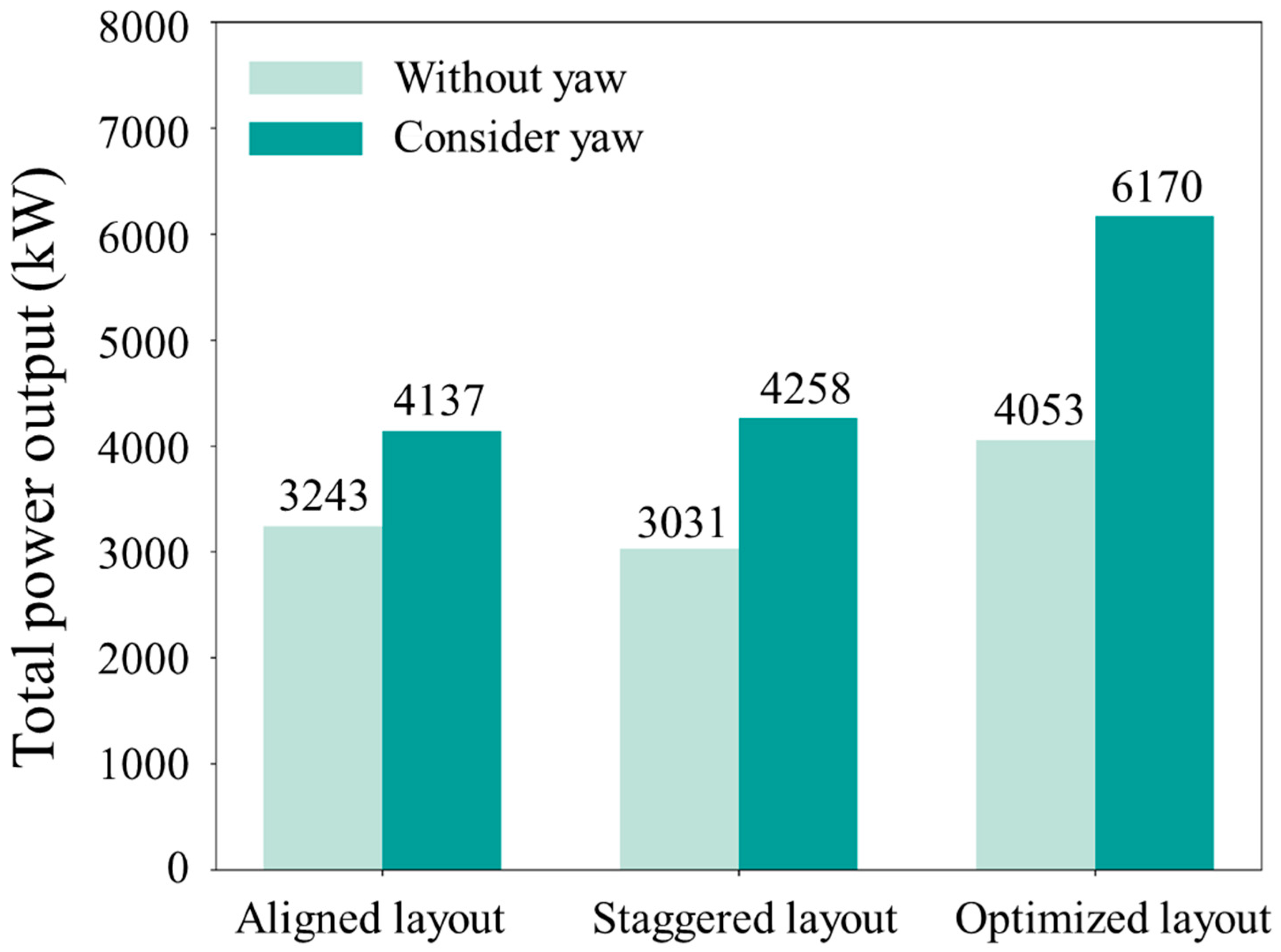
3.3. Effects of Array Layout

Figure 13 shows the total power output for each case with both the aligned and staggered layouts. It can be seen, for both layouts, when the number of turbines is the same, higher power output is achieved in layouts with larger $∆x$ and/or $∆y$. This conclusion is consistent with the findings presented in [36].

The difference between power outputs of the two layouts is calculated as $\left(\left|P_{aligned}-P_{staggered}\right|\right)/P_{aligned}$. As can be seen in Figure 13, the power output of the aligned layout is not always higher than that of the staggered layout. The absolute differences in most cases are less than 5.00%. The highest and lowest differences are 9.57% and 10.93%, respectively, both significantly lower than 53.00% reported in [31], where 12 turbines were deployed in aligned and staggered layouts in an ideal rectangular computational domain. The primary reason for this discrepancy is the direction of the inflow tidal stream. In the ideal case, the inflow velocity is constant and keeps flowing from the left to the right boundary. The staggered layout allows the downstream turbines to extract energy from undisturbed or accelerated tidal stream flowing through the gap between the upstream turbines. However,, in the aligned layout, downstream turbines can only operate in the wake of the upstream turbines. Therefore, the staggered layout exhibits a much higher power output than the aligned layout. However, in real-world scenarios, such as the HP channel, the tidal direction is neither constant across the channel nor over time. Thus, the turbines in the aligned layout of this study are not “purely” aligned. For example, when the inflow tidal stream approaches with a 45$°$ yaw angle, the turbines are actually in a staggered layout. As a result, the differences in power outputs between the aligned and staggered layouts are much less pronounced. Similar results are also reported in [22], where the difference is around 6.54%.

To further study the effect of array layouts, we select four arrays to investigate the flow velocity field around the array. All the four arrays consist of 20 turbines each. Among the four arrays, arrays $A_h$ and $A_l$ are aligned layouts in cases 14 and 21, which have the highest and lowest power outputs, respectively, among the aligned cases with 20 turbines. Arrays $S_l$ and $S_h$ are staggered layouts in cases 8 and 21, which have the lowest and highest power outputs, respectively, among the staggered cases with 20 turbines.

To enhance clarity, we define “upstream” as the south side of the array during flood tide and the north side during ebb tide. The “downstream” is defined as the opposite.

Figure 14 and Figure 15 show the velocity distribution around the turbine array in the four arrays at peak flood and ebb tides, respectively. Comparing to array $A_l$, array $A_h$ decreases $∆x$ to increase the number of turbines per row. There are more upstream turbines, which can extract energy from the undisturbed tidal stream, and fewer downstream turbines are affected by wake flow. In addition, as the direction of the tidal stream is not orthogonal to the x-direction, the turbines in array $A_h$ are actually in a staggered layout, as shown in Figure 15a. Most downstream turbines are not affected by the wake of the upstream turbines at the peak ebb tide in array $A_h$. As a result, the power output of array $A_h$ is higher than that of array $A_l$. As for the staggered layout, even though there are more turbines deployed in the upstream area, the layout of array $S_l$ resembles an aligned layout because of the direction of the tidal stream. However, the layout $S_h$ can still benefit from the staggered layout. Thus, the power output of array $S_h$ is higher than that of array $S_l$.

3.4. Effects of Yaw Angle

In order to investigate the effects of the yaw angle, three arrays $T_A$, $T_S$ and $T_o$, based on the three layouts from [22], are obtained by introducing the yaw angle for each turbine and optimizing the flood and ebb yaw angles through the gradient-based optimization. It should be noted that the performance of arrays $O_A$, $O_S$ and $O_o$ was evaluated using OpenTidalFarm in [22]. As Thetis uses a different finite element method compared to OpenTidalFarm, the solving method may account for causing array performance differences. Therefore, we collect all the turbines’ coordinates data of arrays $O_A$, $O_S$ and $O_o$, and evaluate their performance again using Thetis.

Figure 16 shows the comparison of power output with and without considering yaw angles. It can be seen, for both aligned and staggered layouts, the power outputs are improved significantly after considering the yaw angle. The improvement is around 27.6% from $O_A$ to $T_A$, and 40.5% from $O_S$ to $T_S$. However, regardless of whether yaw angles are considered, the differences between the aligned and staggered layouts are limited to less than 10%, which is consistent with the conclusion from Section 3.3.

The layout $O_o$ takes the turbine coordinates as the optimization parameters, resulting in a final improvement of about 33.7% in array power output compared to $O_S$. However, in layout $T_o$ obtained by optimizing both the turbines’ location and yaw angles, the performance has an additional improvement about 52.5%, more than double the power output of $O_S$. This confirms that not only turbine location, but also the yaw angle of each turbine, can significantly affect array performance.

Figure 17 shows the location of turbines and their corresponding yaw angles during the flood and ebb tides. The velocity distribution around the turbine arrays at the peak flood and ebb tides is also displayed. It is clear that, during both peak flood and ebb tides, turbines located on the east and west sides of the array face the incoming tidal stream at 45$°$ and 135$°$ yaw angles, respectively.

Finally, the shape of $T_A$ and $T_S$ is akin to “\_/”, which aids in directing the stream flow towards the intermediate turbines with a higher velocity. In addition, since the wake of the yawed turbine can be steered, there is less accumulation of turbine wakes. The downstream turbines operate with higher efficiency, as the inflow is nearly undisturbed. Thus, the performance of $T_A$ and $T_S$ is significantly improved compared to $O_A$ and $O_S$.

As for $T_O$, it can be seen in Figure 17e,f that turbines are not restricted to alignment along the x-axis or y-axis. The entire array are now positioned in the north side of the TDA where the tidal stream energy is more abundant [34]. Turbines in $T_O$ now form new rows, with their normal direction aligned parallel to the incoming tidal stream velocity direction. The number of turbines at each new row increases, while the number of rows decreases to around 2. As a result, more upstream turbines can directly extract energy from the undisturbed tidal stream. The downstream turbines can benefit greatly from a local accelerated tidal stream flowing through the gap of the upstream turbines, as the distances between rows decrease. For the downstream turbines at the two sides of the array, their performance is also improved, since the corresponding upstream turbines steer their wake away from the downstream turbines.

Figure 18 displays the instantaneous power outputs (IPOs) of the three layouts, with and without considering the yaw angle. The two peak moments of the IPOs correspond to the peak flood and ebb tides, respectively. When the tidal stream changes its direction, the velocity magnitude approaches zero so that the IPO reaches around zero. It can be observed that, while the yaw angle is not considered, the aligned layout, $O_A$, consistently produces higher IPOs than the staggered layout $O_S$. In cases where the yaw angle is considered, the relationship of the IPO between the aligned and staggered layouts remains consistent during the flood tide. However, the IPO of $T_S$ exceeds that of $T_A$ during the ebb tide. This can be attributed to the fact that the directions of the tidal stream during flood and ebb tides are opposite, but not parallel. The directions form an obtuse angle relative to each other. Thus, when considering the yaw angle, the power output during the ebb tide is significantly improved, resulting in a higher total power output compared to cases where yaw angle effects are ignored.

It can also be found that, when considering the yaw angle, not only is the peak IPO improved, but also the period when the IPO remains at a higher value is increased. For example, the peak IPO of $T_O$ overwhelms that of $O_o$. During the approximately 6 h flood period, the IPO for $T_O$ exceeds 2000 kW for nearly 4 h. In contrast, for $O_o$, the IPO exceeds 2000 kW for only about 1 h. This confirms that the yaw angle is a crucial factor that cannot be ignored during the design of the turbine array layouts. It is, therefore, more effective to optimize the turbine location and yaw angle simultaneously to enhance the array performance.

4. Conclusions

In this study, a two-dimensional hydrodynamic model is set up using Thetis, which is validated with data from an elevation station and a velocity station in the channel between Hulu Island and Putuoshan Island (the HP channel). A yawed tidal stream turbine model, based on the linear momentum actuator disc theory, is then validated using laboratory flume data. Furthermore, a gradient-based optimization model is introduced to enhance turbine array performance. Finally, the validated models are applied to investigate the influence of turbine number, array layouts, and yaw angles on tidal stream turbine array performance.

First, a tidal stream turbine array with varying numbers of turbines is investigated, and the results reveal that the overall power production of the array is positively proportional to the number of turbines. However, the power output per turbine initially increases and then gradually decreases at variable rates.

Second, the performance of turbine arrays with different layouts is compared. When turbines are placed in a practical location, it is found that there may not be any discernible difference between the aligned and staggered layouts, particularly when the turbine row’s normal direction is not parallel to the inflow direction.

Finally, the influence of yaw angles is investigated. The results indicate that, after adjusting for yaw angle, downstream turbines can dramatically benefit from the upstream turbines’ steering wake, leading to a substantial improvement in turbine array performance. Optimizing the turbine position and yaw angle simultaneously can result in a higher array power output than optimizing the yaw angle alone. Furthermore, it must be considered that the yaw angle not only results in a higher peak instantaneous power production than a turbine array without yaw but also maintains high performance for a longer period.

References

1. Dong, Y.; Yan, Y.; Xu, S.; Zhang, X.; Zhang, X.; Chen, J.; Guo, J. An Adaptive Yaw Method of Horizontal-Axis Tidal Stream Turbines for Bidirectional Energy Capture. Energy 2023, 282, 128918. [Google Scholar] [CrossRef]
2. Zhang, D.; Wang, J.; Lin, Y.; Si, Y.; Huang, C.; Yang, J.; Huang, B.; Li, W. Present Situation and Future Prospect of Renewable Energy in China. Renew. Sustain. Energy Rev. 2017, 76, 865–871. [Google Scholar] [CrossRef]
3. Melikoglu, M. Current Status and Future of Ocean Energy Sources: A Global Review. Ocean Eng. 2018, 148, 563–573. [Google Scholar] [CrossRef]
4. Zheng, J.; Dai, P.; Zhang, J. Tidal Stream Energy in China. Procedia Eng. 2015, 116, 880–887. [Google Scholar] [CrossRef]
5. Azlan, F.; Kurnia, J.C.; Tan, B.T.; Ismadi, M.-Z. Review on Optimisation Methods of Wind Farm Array under Three Classical Wind Condition Problems. Renew. Sustain. Energy Rev. 2021, 135, 110047. [Google Scholar] [CrossRef]
6. Vennell, R. The Energetics of Large Tidal Turbine Arrays. Renew. Energy 2012, 48, 210–219. [Google Scholar] [CrossRef]
7. Vennell, R.; Funke, S.W.; Draper, S.; Stevens, C.; Divett, T. Designing Large Arrays of Tidal Turbines: A Synthesis and Review. Renew. Sustain. Energy Rev. 2015, 41, 454–472. [Google Scholar] [CrossRef]
8. Malki, R.; Williams, A.J.; Croft, T.N.; Togneri, M.; Masters, I. A Coupled Blade Element Momentum—Computational Fluid Dynamics Model for Evaluating Tidal Stream Turbine Performance. Appl. Math. Model. 2013, 37, 3006–3020. [Google Scholar] [CrossRef]
9. Chen, Y.; Lin, B.; Lin, J.; Wang, S. Experimental Study of Wake Structure behind a Horizontal Axis Tidal Stream Turbine. Appl. Energy 2017, 196, 82–96. [Google Scholar] [CrossRef]
10. Divett, T.; Vennell, R.; Stevens, C. Optimization of Multiple Turbine Arrays in a Channel with Tidally Reversing Flow by Numerical Modelling with Adaptive Mesh. Phil. Trans. R. Soc. A. 2013, 371, 20120251. [Google Scholar] [CrossRef]
11. Draper, S.; Nishino, T. Centred and Staggered Arrangements of Tidal Turbines. J. Fluid Mech. 2014, 739, 72–93. [Google Scholar] [CrossRef]
12. Nash, S.; Olbert, A.; Hartnett, M. Towards a Low-Cost Modelling System for Optimising the Layout of Tidal Turbine Arrays. Energies 2015, 8, 13521–13539. [Google Scholar] [CrossRef]
13. Lo Brutto, O.A.; Thiébot, J.; Guillou, S.S.; Gualous, H. A Semi-Analytic Method to Optimize Tidal Farm Layouts—Application to the Alderney Race (Raz Blanchard), France. Appl. Energy 2016, 183, 1168–1180. [Google Scholar] [CrossRef]
14. Lo Brutto, O.A.; Nguyen, V.T.; Guillou, S.S.; Thiébot, J.; Gualous, H. Tidal Farm Analysis Using an Analytical Model for the Flow Velocity Prediction in the Wake of a Tidal Turbine with Small Diameter to Depth Ratio. Renew. Energy 2016, 99, 347–359. [Google Scholar] [CrossRef]
15. Wu, G.; Wu, H.; Wang, X.; Zhou, Q.; Liu, X. Tidal Turbine Array Optimization Based on the Discrete Particle Swarm Algorithm. China Ocean Eng 2018, 32, 358–364. [Google Scholar] [CrossRef]
16. Wu, Y.; Wu, H.; Kang, H.-S.; Li, H. Layout Optimization of a Tidal Current Turbine Array Based on Quantum Discrete Particle Swarm Algorithm. J. Mar. Sci. Eng. 2023, 11, 1994. [Google Scholar] [CrossRef]
17. Funke, S.W.; Farrell, P.E.; Piggott, M.D. Tidal Turbine Array Optimisation Using the Adjoint Approach. Renew. Energy 2014, 63, 658–673. [Google Scholar] [CrossRef]
18. Funke, S.W.; Farrell, P.E. A Framework for Automated PDE-Constrained Optimisation. arXiv 2013, arXiv:1302.3894. [Google Scholar]
19. Funke, S. The Automation of PDE-Constrained Optimisation and Its Applications. Ph.D. Thesis, Imperial College London, London, UK, 2013. [Google Scholar]
20. Culley, D.M.; Funke, S.W.; Kramer, S.C.; Piggott, M.D. Integration of Cost Modelling within the Micro-Siting Design Optimisation of Tidal Turbine Arrays. Renew. Energy 2016, 85, 215–227. [Google Scholar] [CrossRef]
21. Du Feu, R.J.; Funke, S.W.; Kramer, S.C.; Hill, J.; Piggott, M.D. The Trade-off between Tidal-Turbine Array Yield and Environmental Impact: A Habitat Suitability Modelling Approach. Renew. Energy 2019, 143, 390–403. [Google Scholar] [CrossRef]
22. Zhang, C.; Zhang, J.; Tong, L.; Guo, Y.; Zhang, P. Investigation of Array Layout of Tidal Stream Turbines on Energy Extraction Efficiency. Ocean Eng. 2020, 196, 106775. [Google Scholar] [CrossRef]
23. Qian, Y.; Zhang, Y.; Sun, Y.; Zhang, H.; Zhang, Z.; Li, C. Experimental and Numerical Investigations on the Performance and Wake Characteristics of a Tidal Turbine under Yaw. Ocean Eng. 2023, 289, 116276. [Google Scholar] [CrossRef]
24. Zhang, Y.; Peng, B.; Zheng, J.; Zheng, Y.; Tang, Q.; Liu, Z.; Xu, J.; Wang, Y.; Fernandez-Rodriguez, E. The Impact of Yaw Motion on the Wake Interaction of Adjacent Floating Tidal Stream Turbines under Free Surface Condition. Energy 2023, 283, 129071. [Google Scholar] [CrossRef]
25. Galloway, P.W.; Myers, L.E.; Bahaj, A.S. Experimental and Numerical Results of Rotor Power and Thrust of a Tidal Turbine Operating at Yaw and in Waves. In Proceedings of the World Renewable Energy Congress, Linköping, Sweden, 8–13 May 2011; p. 2246e2253. [Google Scholar]
26. Zhang, C.; Zhang, J.; Angeloudis, A.; Zhou, Y.; Kramer, S.C.; Piggott, M.D. Physical Modelling of Tidal Stream Turbine Wake Structures under Yaw Conditions. Energies 2023, 16, 1742. [Google Scholar] [CrossRef]
27. Li, C.; Zhang, Y.; Zheng, Y.; Qian, Y.; Fernandez-Rodriguez, E.; Benini, E. Research on the Effect of Yawing Motion on Tidal Turbine Performance Based on Actuator-Line Method. Ocean Eng. 2023, 279, 114345. [Google Scholar] [CrossRef]
28. Modali, P.K. On Performance and Wake Characteristics of a Tidal Turbine under Yaw; Lehigh University: Bethlehem, PA, USA, 2016. [Google Scholar]
29. Badoe, C.E.; Li, X.; Williams, A.J.; Masters, I. Output of a Tidal Farm in Yawed Flow and Varying Turbulence Using GAD-CFD. Ocean Eng. 2024, 294, 116736. [Google Scholar] [CrossRef]
30. Kramer, S.C.; Piggott, M.D. A Correction to the Enhanced Bottom Drag Parameterisation of Tidal Turbines. Renew. Energy 2016, 92, 385–396. [Google Scholar] [CrossRef]
31. Zhang, C.; Kramer, S.C.; Angeloudis, A.; Zhang, J.; Lin, X.; Piggott, M.D. Improving Tidal Turbine Array Performance through the Optimisation of Layout and Yaw Angles. Int. J. Mar. Ene. 2022, 5, 273–280. [Google Scholar] [CrossRef]
32. Schwedes, T.; Ham, D.A.; Funke, S.W.; Piggott, M.D. Mesh Dependence in PDE- Constrained Optimisation; Springer International Publishing: Berlin/Heidelberg, Germany, 2017. [Google Scholar]
33. Zhang, J.; Zhang, C.; Angeloudis, A.; Kramer, S.C.; He, R.; Piggott, M.D. Interactions between Tidal Stream Turbine Arrays and Their Hydrodynamic Impact around Zhoushan Island, China. Ocean Eng. 2022, 246, 110431. [Google Scholar] [CrossRef]
34. Zhang, C.; Cheng, X.; Angeloudis, A.; Kramer, S.C.; Wu, C.; Chen, Y.; Piggott, M.D. Economics-Constrained Tidal Turbine Array Layout Optimisation at the Putuoshan–Hulu Island Waterway. Ocean Eng. 2024, 314, 119618. [Google Scholar] [CrossRef]
35. Egbert, G.D.; Erofeeva, S.Y. Efficient Inverse Modeling of Barotropic Ocean Tides. J. Atmos. Ocean. Technol. 2002, 19, 183–204. [Google Scholar] [CrossRef]
36. O’Doherty, D.M.; Mason-Jones, A.; Morris, C.; O’Doherty, T.; Byrne, C.; Prickett, P.W.; Grosvenor, R.I. Others Interaction of Marine Turbines in Close Proximity. In Proceedings of the 9th european wave and tidal energy conference (EWTEC), Southampton, UK, 5–9 September 2011; pp. 10–14. [Google Scholar]
Figure 1. The yawed turbine approximated through the enhanced bottom friction using the linear momentum actuator disc theory [30].
Jmse 12 02325 g001
Figure 2. The mesh of the computational domain. The red rectangular shaped area in the enlarged frame shows the Turbine Deploying Area.
Jmse 12 02325 g002
Figure 3. The water depth distribution around Hulu Island. The elevation station is marked with green circle and “A” text, and the tidal velocity station is marked with blue circle and “B” text.
Jmse 12 02325 g003
Figure 4. Experimental set up at the circulating flow flume. (a) the porous walls at the inlet of the flume. (b) the downward-facing Nortek Vectrino Profiler positioned on a movable platform behind the turbine.
Jmse 12 02325 g004
Figure 5. Structure of the sampling points in the turbine wake area.
Jmse 12 02325 g005
Figure 6. Definition of yaw angle θ in the realistic area.
Jmse 12 02325 g006
Figure 7. The schematic diagram of turbine array layout: (a) the aligned layout, (b) the staggered layout.
Jmse 12 02325 g007
Figure 8. The three turbine layouts from Zhang et al. [22].
Jmse 12 02325 g008
Figure 9. Comparison between measured and simulated tidal elevation at tidal elevation station A.
Jmse 12 02325 g009
Figure 10. Comparison between measured and simulated tidal elevation at tidal velocity station B: (a) tidal velocity magnitude; (b) tidal velocity direction.
Jmse 12 02325 g010
Figure 11. The validation results of single turbine’s wake velocity distribution under different yaw angles: (a) 0 ° , (b) 10 ° , (c) 20 ° , (d) 30 ° .
Jmse 12 02325 g011
Figure 12. The power output with different number of turbines. (a) total power output in aligned layout, (b) power output per turbine in aligned layout, (c) total power output in staggered layout, (d) power output per turbine in staggered layout.
Jmse 12 02325 g012
Figure 13. The total power outputs among the 25 cases and the differences between the aligned layout and staggered layout for each case.
Jmse 12 02325 g013
Figure 14. The schematic diagram of velocity distribution around turbine array in layouts A h , A l , S l , and S h at the peak flood tide.
Jmse 12 02325 g014
Figure 15. The schematic diagram of velocity distribution around turbine array in layouts A h , A l , S l , and S h at the peak ebb tide.
Jmse 12 02325 g015
Figure 16. The power outputs of three layouts with and without considering yaw angle.
Jmse 12 02325 g016
Figure 17. The velocity distribution around the arrays T A , T S , and T o during the peak spring and ebb tides.
Jmse 12 02325 g017
Figure 18. The instantaneous power outputs of arrays O A , O S , O o , T A , T S , and T o during the intermediate tide.
Jmse 12 02325 g018