An Improved D* Lite-Based Dynamic Route Planning Algorithm for Ships in Arctic Waters

Abstract

The ice conditions in Arctic waters are complex and variable, requiring ships to dynamically adjust their routes to ensure safe and efficient navigation. Traditional dynamic path planning algorithms struggle to address the extensive variability of Arctic ice conditions. To tackle this issue, this paper improves the D* Lite algorithm by leveraging the gradual and convergent nature of Arctic ice condition changes. The original algorithm’s local update and path extraction rules are modified to prevent chain updates triggered by minor localized changes, thereby reducing the frequency of updates in non-critical areas. By simulating dynamic route planning for ships in Arctic waters during both the freezing and melting periods, the improved D* Lite algorithm was compared with the original D* Lite algorithm and a global update algorithm in terms of voyage distance, risk coefficient, planning time, and the number of node updates. The computational results demonstrate that the improved D* Lite algorithm achieves planning results very similar to those of the original D* Lite algorithm and the global update algorithm at the lowest update cost, significantly enhancing the safety and efficiency of dynamic route planning for ships in Arctic waters.

1. Introduction

In recent years, intensified global warming has significantly improved navigation conditions in the Arctic Ocean, extending the navigation window period. Additionally, driven by geopolitical factors, the risks and transportation costs associated with shipping in several traditionally busy international trade routes have been steadily rising [1]. These developments have underscored the immense economic potential for the development of Arctic shipping routes [2], while also providing new guarantees for the stable development of the shipping industry. However, the Arctic Ocean exhibits complex and unpredictable ice conditions, and the current time span of ice forecasts does not meet the requirements for the initial route planning of a vessel over its entire voyage, presenting significant challenges during the actual navigation of vessels in Arctic waters [3,4]. Therefore, effectively utilizing the latest ice condition data to achieve real-time route planning for vessels in transit has remained a focal point of research.

In the study of vessel route planning in Arctic waters, the risks and costs associated with icebreaking are crucial and cannot be neglected. Through various methods such as the Analytic Hierarchy Process [5], comprehensive evaluation [6], gray relational analysis [7], and dynamic Bayesian networks [8,9], a substantial body of research has identified the main environmental factors influencing the safety and efficiency of vessel navigation in Arctic waters. As shown in

Table 1. Overview of Arctic route planning related research.

Correlative Papers	Environmental Factors	Ship Performance Model	Route Planning Algorithm
Kotovirta et al., 2009 [13]	Sea ice concentration, thickness	Semi-empirical formula	Powell’s method
Nam et al., 2013 [14]	Sea ice concentration, thickness, temperature, current, salinity	Numerical simulation	Dijkstra algorithm
Choi et al., 2015 [15]	Sea ice concentration, thickness, air pressure, temperature, wind speed, velocity	Semi-empirical formula	A* algorithm
Zhang et al., 2019 [16]	Sea ice concentration, thickness, wind speed, wave height, temperature, water temperature	Data-driven	Ant colony algorithm
Topaj et al., 2019 [17]	/	Semi-empirical formula	Equivalent waveform graph
Lehtola et al., 2019 [18]	Sea ice concentration, thickness	Semi-empirical formula	A* algorithm
Lee et al., 2021 [19]	Sea ice concentration, thickness, wind speed, velocity, water depth, temperature	Numerical simulation	Seed genetic algorithm
Zhang et al., 2022 [20]	Sea ice concentration, thickness, wind speed, velocity	Semi-empirical formula	3D Ant colony algorithm
Li et al., 2022 [9]	Sea ice concentration, temperature, wind speed, wave height	/	A* algorithm
Shu et al., 2023 [21]	Sea ice concentration, thickness	Numerical simulation	Equivalent waveform graph
Li et al., 2024 [22]	Sea ice concentration	/	Velocity obstacle algorithm

, most studies have considered sea ice thickness and sea ice concentration as key environmental factors. While satellite observation technology has enhanced sea ice concentration forecasting, sea ice thickness remains less accurate due to its higher observation difficulty during months of significant ice changes. Meanwhile, ice resistance serves as the primary source of drag for vessels navigating through Arctic waters and is a significant factor influencing navigation efficiency. Current research methods for ice resistance mainly include semi-empirical formulas [10], numerical simulations [11], and data-driven approaches [12]. These methods ultimately apply the derived formulas to the calculation of route planning, with the accuracy of their results positively correlating with the complexity of the formulas. Consequently, avoiding redundant calculations of irrelevant nodes is crucial for achieving efficient real-time ship route planning.

Given that ice condition data are typically gridded, Arctic vessel route planning studies often rely on raster maps [23]. For instance, Nam et al. [14] utilized an ice-coupled ocean general circulation model (OGCM) to simulate the distribution and variation in sea ice in the Arctic Ocean, employing Dijkstra’s algorithm to calculate the lowest total cost route among predefined waypoints. Choi et al. [15] integrated uncertainty in ice conditions into their cost calculations and used the A* algorithm for initial route planning. Lehtola et al. [18] considered ship speeds and ice entrapment probabilities for different ice thicknesses, using the A* algorithm to output a set of routes that follow the curvature of the Earth. Although graph-search path planning algorithms based on node searches have been widely applied in Arctic vessel route planning studies, their limitations in path planning are evident: the planned paths often exhibit a “jagged” appearance, deviating from the actual optimal path. To enhance the effectiveness of graph-search algorithms in route planning, researchers often optimize by increasing the map resolution, using multi-neighborhood searches, and applying smoothing processes [24,25]. It is noteworthy that existing studies on Arctic vessel route planning primarily focus on static initial route planning, and while some dynamic planning schemes utilize static planning algorithms for global replanning, they have not truly achieved efficient dynamic route planning.

An in-depth review of the existing literature on Arctic vessel route planning reveals trends and shortcomings: (1) As research on risk and performance models for ships navigating in ice-covered waters deepens, the factors considered in relevant studies have become increasingly comprehensive. On the one hand, it has enhanced the accuracy and safety of route planning; however, on the other hand, it has inevitably increased computational complexity, which poses a significant challenge to the efficiency of real-time route planning for vessels in Arctic waters. (2) Currently, research on vessel route planning in Arctic waters primarily focuses on using graph-search algorithms for static initial route planning. However, due to limitations in ice forecasting capabilities and insufficient data accuracy in Arctic waters, these studies cannot guarantee the effectiveness of routes over the entire voyage. This status quo indicates that effectively integrating dynamic route planning algorithms into the research on vessel route planning in Arctic waters to achieve dynamic route planning for the entire voyage will become a new research focus. To address these challenges, this paper proposes a dynamic route planning method based on an improved D* Lite algorithm, adapted to Arctic ice conditions for minimal-cost dynamic updates.

2. Algorithm

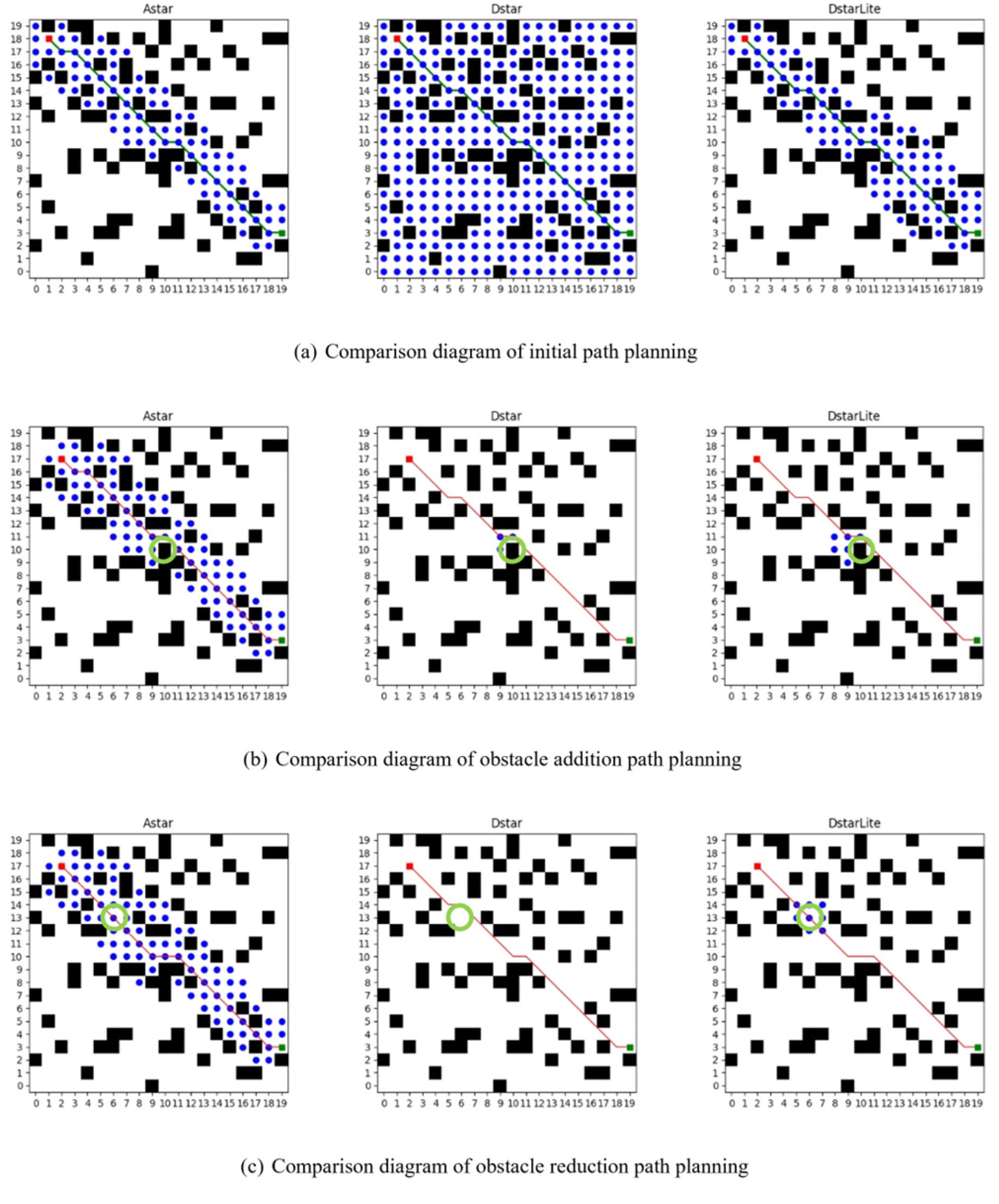
Dynamic route planning for ships in Arctic waters necessitates the ability to address complex changes in ice conditions to ensure the effectiveness of the path throughout the navigation process. Figure 1a–c depict the path planning results of three algorithms—A*, D*, and D* Lite—across three scenarios: initial map, addition of obstacle points, and the removal of obstacle points from the map.

In this context, the addition and removal of obstacle points correspond to the freezing and melting periods in Arctic waters, respectively. Within the figure: the red points denote the starting position, the green points denote the destination, the green line segments represent the initial path, and the red line segments indicate the updated paths following changes in obstacle points. The locations of altered obstacle points are indicated by green circles. The results presented demonstrate that current mainstream graph search path planning algorithms exhibit certain shortcomings when applied to route planning for ships in Arctic waters. For instance, the A* algorithm lacks the capability to reuse historical data, the D* algorithm only performs dynamic planning when new obstacle points arise along the current path, and the D* Lite algorithm can adapt to changes in the navigation areas during both the freezing and melting periods in the Arctic.

2.1. D* Lite Algorithm

The D* Lite algorithm [26] is a dynamic path planning algorithm proposed by Sven Koenig and Maxim Likhachev in 2002, which is an improvement based on the LPA* [27] and D* [28] algorithms. This algorithm combines the incremental update strategy of the LPA* algorithm with the reverse search design of the D* algorithm, enabling dynamic path planning with a reduced computational cost.

Similarly to most graph search path planning algorithms, the D* Lite algorithm achieves path planning by calculating and updating the actual minimum cost values $g\left(s\right)$ from each node to the destination. As the algorithm needs to handle the changes in the $g\left(s\right)$ values of nodes due to variations in the map environment, it introduces an estimated minimum cost value $\mathit{rhs}\left(s\right)$. During the path update process, the $\mathit{rhs}\left(s\right)$ value of nodes is updated first; if $\mathit{rhs}\left(s\right)$ is less than $g\left(s\right)$, it is assigned to $g\left(s\right)$. The specific formulas for $g\left(s\right)$ and $\mathit{rhs}\left(s\right)$ are as follows:

$$g\left(s\right)=\mathit{rhs}\left(s\right)=\left\{\begin{array}{c}0,\hspace{1em}\hspace{1em}\hspace{1em}\hspace{1em}\hspace{1em}\hspace{1em}\hspace{1em}\hspace{1em}\hspace{1em}\hspace{1em}\hspace{1em}\hspace{1em}\mathrm{if} s = s_{\mathit{start}}\hfill \\ \underset{s^{\prime }\in \mathit{Suss} \left(s\right)}{min}c\left(s^{\prime },s\right)+g\left(s^{\prime }\right), \mathrm{o}\mathrm{t}\mathrm{h}\mathrm{e}\mathrm{r}\mathrm{w}\mathrm{i}\mathrm{s}\mathrm{e}\end{array}\right.,$$

(1)

where $s$ is the current point, $s^{\prime }$ is the neighboring node of $s$, $\mathit{Suss}\left(s\right)$ denotes the set of successor nodes of point $s$, and $c\left(s^{\prime },s\right)$ represents the moving cost between point $s$ and its neighboring point $s^{\prime }$.

To enhance the efficiency of path planning, the algorithm iteratively identifies and updates the most likely optimal path nodes from the update queue $U$. The update priority of nodes within the algorithm is determined by its corresponding key value $Key$; a lower $Key$ indicates a higher probability of being an optimal path node, thus prioritizing its update. The path planning process involves adding nodes to the queue $U$, updating $Key$ values in the queue, or removing nodes from the queue. The expression for the update queue $U$ and the calculation formula for the key value $Key$ are as follows:

$$U=\left\{\left({Key}_1,s_i\right),\left({Key}_2,s_j\right)\dots \left({Key}_n,s_k\right)\right\},\left({\mathrm{Key}}_1<{Key}_2<\dots <{Key}_n\right),$$

(2)

where each node $s$ has a corresponding key value $Key$. The $Key$ consists of $k_1$ and $k_2$; when $k_1$ values are equal, $k_2$ values are compared instead. The specific calculation formula for the key value is as follows:

$$Key=\left[\begin{array}{c}{k}_1\\ k_2\end{array}\right]=\left[\begin{array}{c}\min \left(g\left(s\right),\mathit{rhs}\left(s\right)\right)+h\left(s,s_{\mathit{start}}\right)+k_m\\ \min \left(g\left(s\right),\mathit{rhs}\left(s\right)\right)\end{array}\right],$$

(3)

where $h\left(s,s_{\mathit{start}}\right)$ is the heuristic value representing the estimated cost from node $s$ to the starting point, and $k_m$ is a modifier key value denoting the historical moving cost from the start point to the current point.

In the initial path planning, to improve planning efficiency, the heuristic function $h\left(s,s_{\mathit{start}}\right)$ is introduced during the calculation of the node key value $Key$, enabling a “directional” path search. However, when the starting point $s_{\mathit{start}}$ changes, the subsequent updates of node $Key$ values are based on the new $s_{\mathit{start}}$, leading to inaccuracies in the priority of nodes in the update queue $U$ and insufficient utilization of previous data. To address this issue, the D* Lite algorithm introduces the modifier key value $k_m$ to ensure that nodes are rationally ordered in the update queue $U$ during path updates. The specific calculation formula for $k_m$ is as follows:

$$k_m{=k}_m+h\left(s_{\mathit{last}},s_{\mathit{start}}\right),$$

(4)

where $h\left(s_{\mathit{last}},s_{\mathit{start}}\right)$ represents the heuristic value between the new starting point and the old starting point.

In summary, the D* Lite algorithm has the potential to effectively respond to changes in navigable environments. Compared to other graph search algorithms, it exhibits greater applicability in ship route planning in Arctic waters. However, in scenarios where the navigable environment experiences large-scale changes, even minor alterations can necessitate extensive updates within the algorithm. Such updates may result in dynamic planning processes that approach the complexity of complete re-planning, and in extreme cases, could lead to pathfinding failures. Therefore, to enable the D* Lite algorithm to be applied to ship route planning in Arctic waters, it is critical to thoroughly consider the characteristics of ice condition changes in the Arctic and to develop corresponding enhancements to the algorithm. These improvements are essential for increasing its adaptability and robustness in complex environmental changes.

2.2. Optimization of Local Update Algorithm

The changes in ice conditions in Arctic waters are typically large-scale, which presents significant challenges for the application of the original D* Lite algorithm in this region. Due to these extensive changes in the overall environment, a considerable number of nodes require updates. Consequently, the computational burden during local updates can approach that of global re-planning, potentially leading to pathfinding failures. To reduce updates to non-critical nodes, the improved algorithm flexibly selects either to update the cost of nodes or simply mark them as non-navigable areas based on changes in regional navigability. This approach effectively reduces unnecessary update calculations for irrelevant nodes, specifically as illustrated in Equation (5):

$$\mathrm{Update} \left(S_{key}\right)\left\{\begin{array}{c}\mathrm{u}\mathrm{p}\mathrm{d}\mathrm{a}\mathrm{t}\mathrm{e} S_{key} and S_{key}\prime \mathrm{i}\mathrm{n} \mathrm{o}\mathrm{l}\mathrm{d}\_\mathrm{d}\mathrm{a}\mathrm{t}\mathrm{e}\hspace{1em}\hspace{1em}\hspace{1em}\hspace{1em}\hspace{1em}\hspace{1em}\hspace{1em}\hspace{1em},\mathrm{i}\mathrm{f} S_{key} \mathrm{i}\mathrm{n} \mathrm{n}\mathrm{e}\mathrm{w}\_\mathrm{o}\mathrm{b}\mathrm{s}\\ \mathrm{u}\mathrm{p}\mathrm{d}\mathrm{a}\mathrm{t}\mathrm{e} S_{key} \mathrm{i}\mathrm{n} \mathrm{n}\mathrm{e}\mathrm{w}\_\mathrm{d}\mathrm{a}\mathrm{t}\mathrm{e} \mathrm{t}\mathrm{h}\mathrm{e}\mathrm{n} S_{key}\prime \mathrm{i}\mathrm{n} \mathrm{o}\mathrm{l}\mathrm{d}\_\mathrm{d}\mathrm{a}\mathrm{t}\mathrm{a}\hspace{1em},\mathrm{e}\mathrm{l}\mathrm{s}\mathrm{e}\hfill \end{array}\right.,$$

(5)

where $S_{key}$ represents the key nodes where navigability changes occur; $S_{key}\prime$ denotes the other nodes affected by these key nodes that require cost value updates; $\mathrm{old}\_\mathrm{date}$ and $\mathrm{new}\_\mathrm{date}$, respectively, represent the old and new environmental data; and $\mathrm{new}\_\mathrm{obs}$ denotes the set of new obstacle points.

As shown in Algorithm 1, when a node triggering a local update corresponds to a new obstacle point, the affected nodes will update their cost values using old environmental data to bypass the new obstacle. Conversely, if the node triggering the update is a new navigable point, its cost value will be updated using new environmental data, while the affected nodes will still use old environmental data for their cost value updates. This enhancement allows the D* Lite algorithm to reduce updates to non-critical nodes to some extent while correctly preserving the differences in ice conditions across adjacent regions.

Algorithm 1. Local update algorithm.
Input:	$\mathrm{new}\_\mathrm{obs}$$, \mathrm{old}\_\mathrm{obs}$$, \mathrm{old}\_\mathrm{data}$
Output:	$\mathrm{new}\_\mathrm{date}$
1	nodes = (new_obs - old_obs) | (old_obs - new_obs)
2	for node in nodes:
3	$\hspace{1em}\mathbf{if} \mathrm{node} \mathrm{in} \mathrm{new}\_\mathrm{obs}$:
4	$\hspace{1em}\hspace{1em}\mathrm{new}\_\mathrm{date}$$\left[\mathrm{node}\right]=\mathrm{old}\_\mathrm{data}$ [node]
5	$\hspace{1em}\hspace{1em}\mathrm{new}\_\mathrm{date}$$[\mathrm{node}\prime \in \mathit{Succ}\left(node\right)$$]=\mathrm{old}\_\mathrm{data}$ [node’]
6	elif node in old_obs:
7	$\hspace{1em}\hspace{1em}\mathrm{new}\_\mathrm{date}$ [node] = update(node)
8	$\hspace{1em}\hspace{1em}\mathrm{new}\_\mathrm{date}$$[\mathrm{node}\prime \in \mathit{Succ}\left(node\right)$$]=\mathrm{old}\_\mathrm{data}$ [node’]
9	return new_data

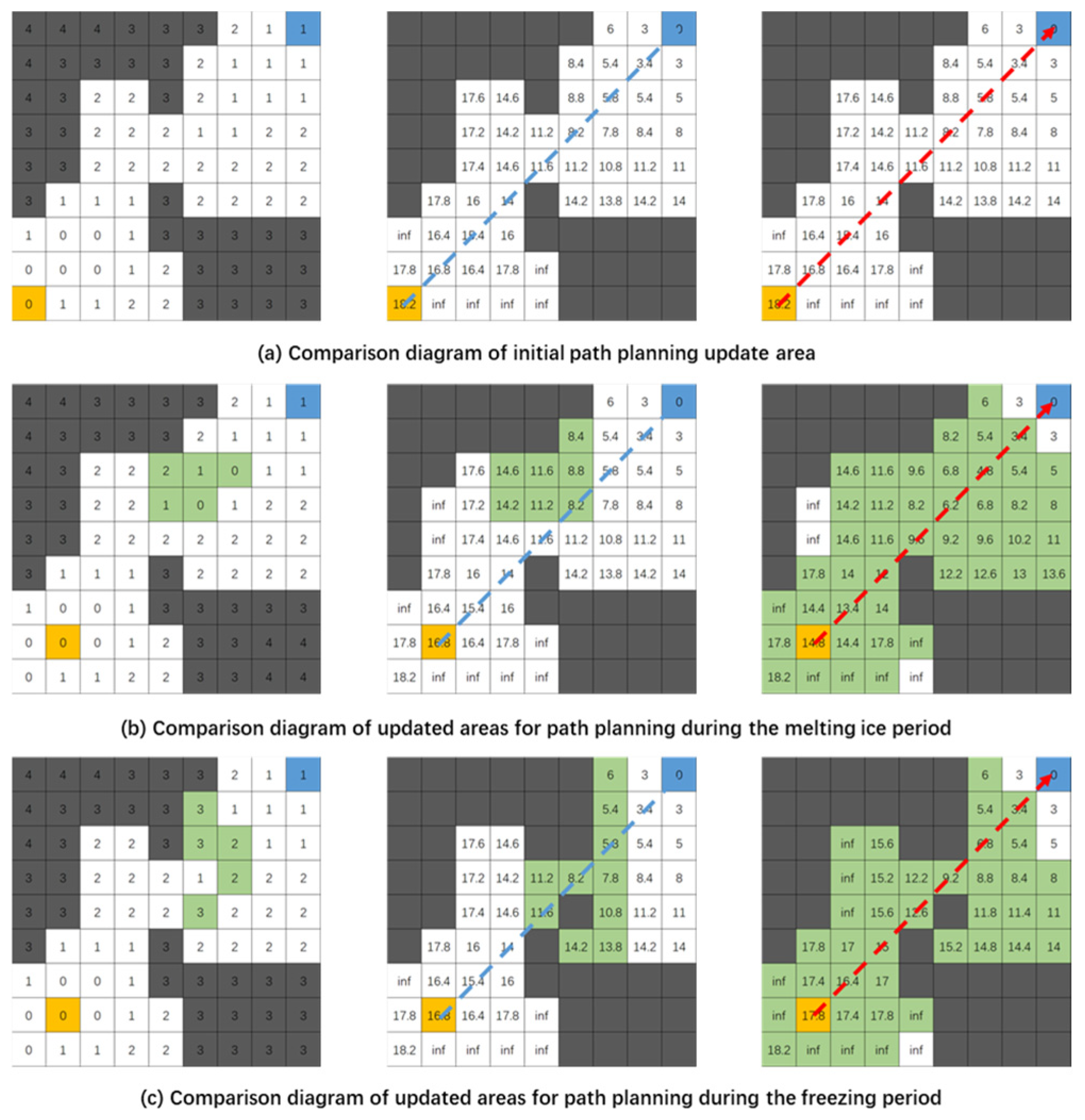
Considering the distinct ice conditions in Arctic waters, categorized into freezing and melting periods [29], the algorithm improvement must address these two scenarios. Figure 2a–c illustrate the route planning results before and after the algorithm improvements under three scenarios: initial ice conditions, melting ice period, and freezing ice period. In each subplot, the first image from the left records the cost values of each node under the current ice conditions. The second and third images, respectively, record the updated actual minimum cost values $g\left(s\right)$ for each node under the improved algorithm and the original algorithm for the given ice conditions. Nodes with cost values greater than 3 are considered obstacle points (gray), orange nodes represent the starting point, blue nodes represent the endpoint, and green areas indicate nodes that have either undergone changes in cost values or been updated by the algorithm. Changes in the route before and after the updates are marked with red and blue directed lines in the figures.

Through simulations of route updates before and after the algorithm improvement under two scenarios of ice condition changes; i.e., during the melting period and the freezing period, it is evident that the improved D* Lite algorithm significantly reduces the number of node updates compared to the original D* Lite algorithm. By identifying critical nodes (regions with navigability changes) and flexibly adopting cost value update strategies based on the characteristics of these changes, the proposed approach effectively avoids “explosive” updates caused by widespread minor variations. This ensures that the improved algorithm achieves efficient dynamic route planning under varying ice conditions in Arctic waters.

2.3. Optimization of Path Extraction Algorithm

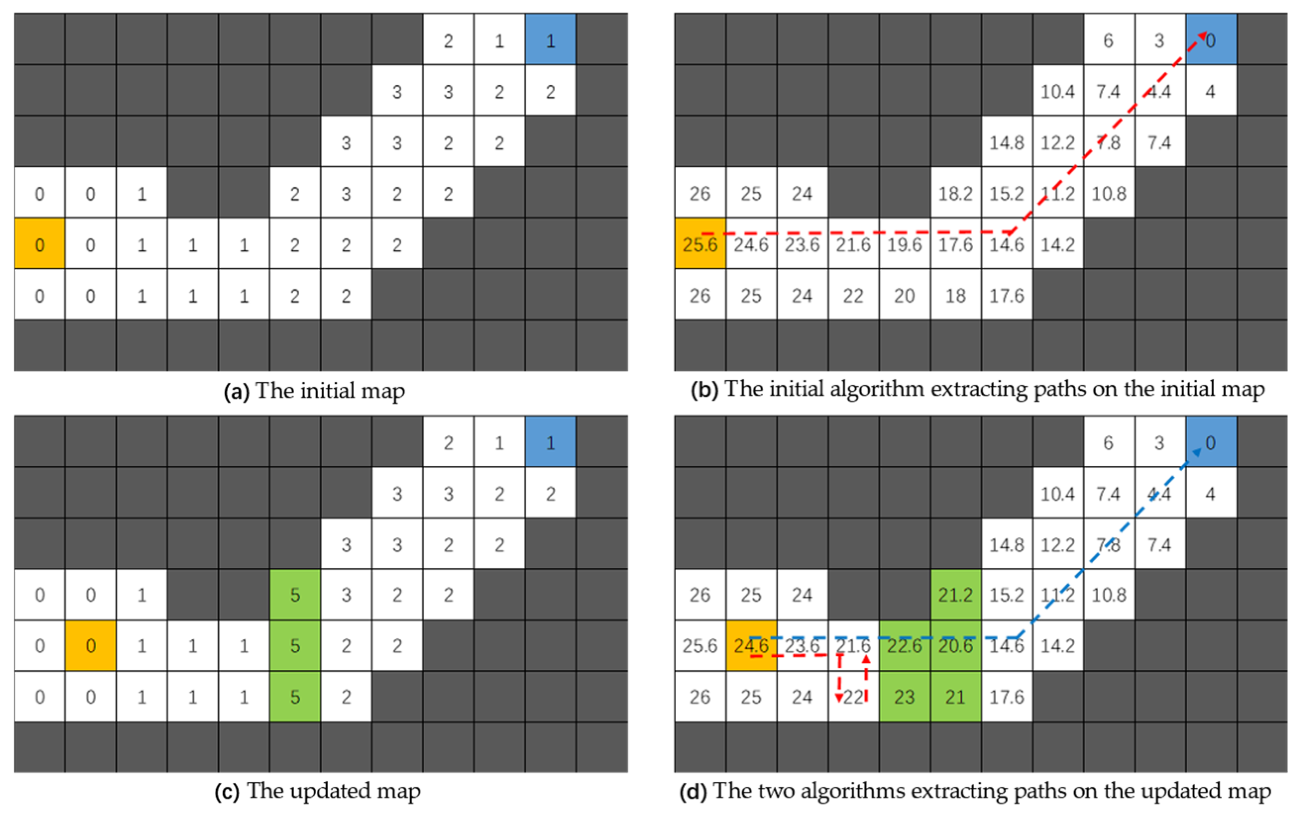
The path extraction logic of the original D* Lite algorithm involves, following the completion of node cost calculations, starting from the initial node and iteratively selecting the surrounding node with the lowest actual cost value as the next path node. This approach is effective when all nodes’ passage cost values are equal. However, in Arctic waters, where ice conditions vary across different regions, the density and average thickness of sea ice differ, leading to fluctuations in the passage cost value associated with icebreaking navigation [30]. For instance, as illustrated in Figure 3, Figure 3a,c indicate the passage cost values of different grids before and after changes in the map environment, while Figure 3b,d show the actual minimum cost values for reaching the destination from different grids under the corresponding environments. The orange grids represent the starting position, while the blue grids represent the destination. After updating the local node passage cost values and actual minimum cost values (green area grids), there may be instances at the boundary between the updated and non-updated areas where the actual minimum cost value of predecessor nodes is higher than that of successor nodes. This situation can lead to a deadlock in the path extraction process (indicated by the red lines in Figure 3b. By incorporating additional consideration of the travel cost between the current node and its neighboring nodes, and excluding the already explored neighboring nodes, the optimal path was successfully extracted (represented by the blue lines in Figure 3d).

To prevent the path extraction process from getting stuck in a deadlock, this paper modifies the rules of the original path extraction algorithm. The primary improvements are reflected in Equation (6) and can be summarized into the following two points:

$$s_{\mathit{new}}={\mathit{argmin}}_{s_{\mathit{opt}}\in \mathit{Succ}\left(s_{\mathit{last}}\right)\cap \mathit{New}}\left(c\left(s_{\mathit{last}},s_{opt}\right)+g\left(s_{opt}\right)\right),$$

(6)

where $s_{\mathit{new}}$ represents the successor node of the current node, $s_{\mathit{last}}$ denotes the current node, $New$ indicates the set of unexplored nodes, and $s_{opt}$ represents the unexplored nodes surrounding the current node. The specific path extraction logic is shown in Algorithm 2.

Algorithm 2. Path extraction algorithm.
Input:	$s_{\mathit{start}}$$, s_{\mathit{goal}}$
Output:	path
1	$\mathrm{path}=[s_{\mathit{start}}$$], New$ = []
2	$s_{\mathit{last}}$$=s_{\mathit{start}}$
3	$\mathbf{while} s_{\mathit{new}}$$!=s_{\mathit{goal}}$:
4	$\hspace{1em}{s}_{\mathit{new}}={\mathit{argmin}}_{s_{\mathit{opt}}\in \mathit{Succ}\left(s_{\mathit{last}}\right)\cap \mathit{New}}\left(c\left(s_{\mathit{last}},s_{opt}\right)+g\left(s_{opt}\right)\right)$:
5	$\hspace{1em}\mathrm{put} \mathrm{all} s_{opt}$$\mathrm{in} New$
6	$\hspace{1em}\mathrm{path}.\mathrm{append}(s_{\mathit{new}}$)
7	return path

2.4. Path Optimization Algorithm

To further enhance the optimality of the improved algorithm in path planning and reduce the probability of falling into a local optimum due to a limited number of updated nodes, an optimization algorithm is introduced to refine the original route planning results. In the original route planning results, certain key nodes are pivotal in determining the optimization outcomes. For two original routes that contain the same key nodes, despite any initial differences, the optimized results will invariably be the same. To ascertain the potential for optimization between two nodes, it is necessary to first compute the cost value of the initial path between these nodes and the cost value of the direct connection path. The formula for calculating the total cost value ${\mathrm{C}\mathrm{o}\mathrm{s}\mathrm{t}}_{ori}$ of any segment of the initial path is provided as follows:

$${\mathrm{C}\mathrm{o}\mathrm{s}\mathrm{t}}_{ori}=\sum _{i=1}^n\mathrm{cost}\left(S_i,S_{i+1}\right),$$

(7)

where $\mathrm{cost}\left(S_i,S_{i+1}\right)$ denotes the cost between points $S_i$ and $S_{i+1}$, calculated as follows:

$$\mathrm{cost}\left(S_i,S_{i+1}\right)={\displaystyle \frac{{\mathrm{Cost}}_{\mathrm{single}}{S}_i+{\mathrm{Cost}}_{\mathrm{single}}{S}_{i+1}}{2}},$$

(8)

where ${\mathrm{Cost}}_{\mathrm{single}}{S}_i$ represents the cost value of node $S_i$, and ${\mathrm{Cost}}_{\mathrm{single}}{S}_{i+1}$ denotes the cost value of node $S_{i+1}$.

The cost value ${\mathrm{C}\mathrm{o}\mathrm{s}\mathrm{t}}_{opt}$ for the direct connection path between any two nodes in the initial path can be calculated with the following formula:

$${\mathrm{C}\mathrm{o}\mathrm{s}\mathrm{t}}_{opt}=\sum _{i=1}^n{\mathrm{C}\mathrm{o}\mathrm{s}\mathrm{t}}_{\mathrm{single}}{S}_i\cdot d,$$

(9)

where $d$ represents the length of the connection within the grid point $S_i$.

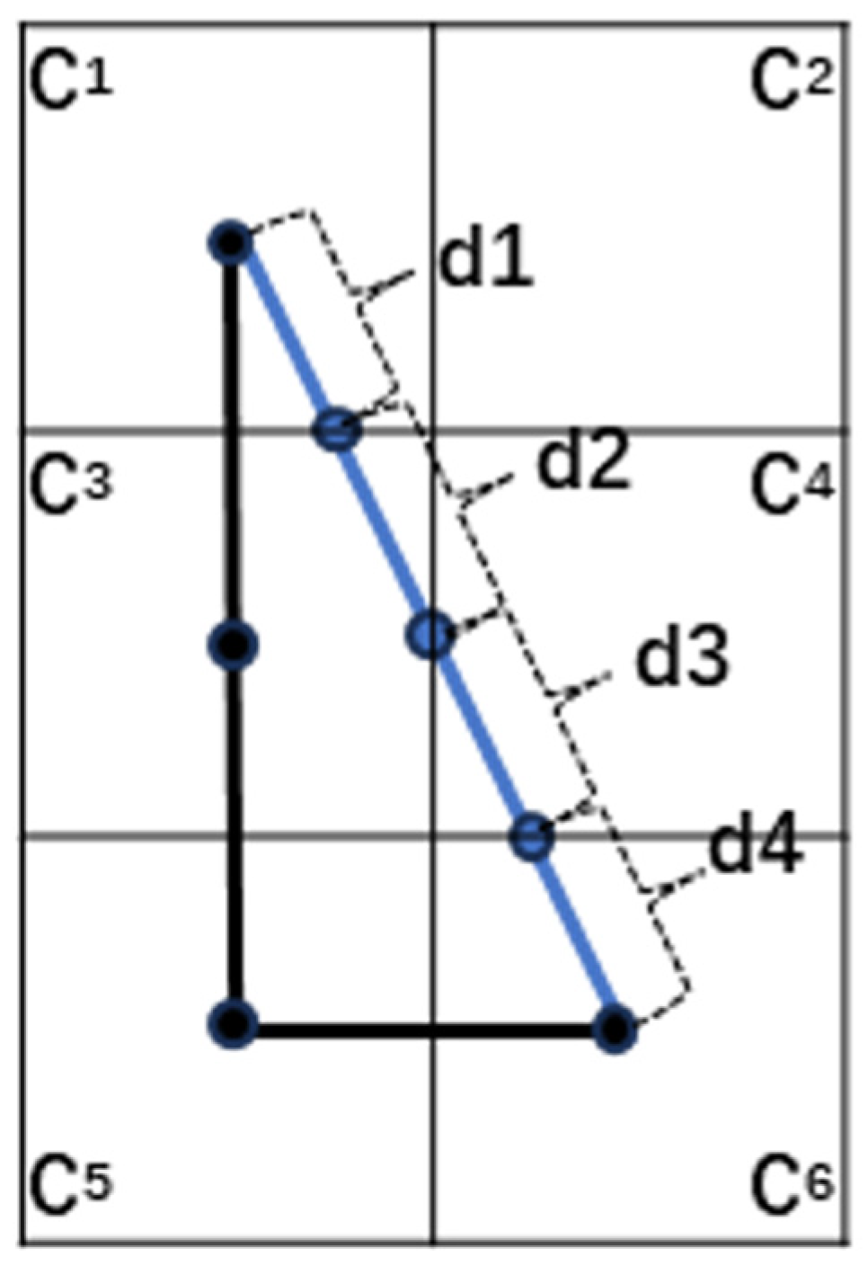
If ${\mathrm{C}\mathrm{o}\mathrm{s}\mathrm{t}}_{opt}$ is less than ${\mathrm{C}\mathrm{o}\mathrm{s}\mathrm{t}}_{ori}$ and the connection does not encounter obstacles, it indicates that the direct connection cost is lower than the initial path, suggesting potential for optimization. By iteratively identifying such nodes and optimizing the connections, the algorithm determines the optimal path. Figure 4 illustrates the navigation costs, which are calculated as $C_1\times d_1+C_3\times d_2+C_4\times d_3+C_6{\times d}_4$.

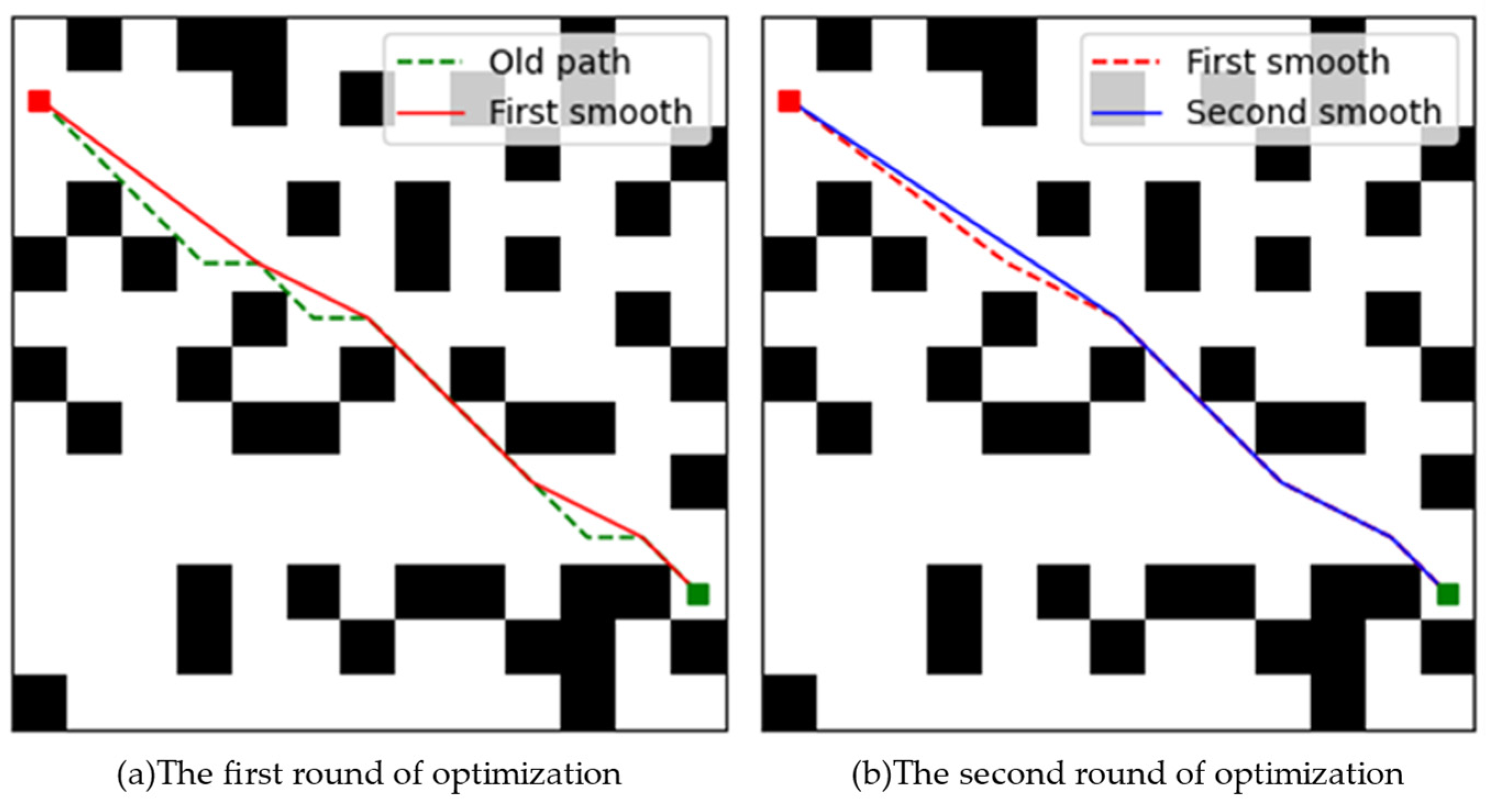
For easier understanding and visual representation, under the assumption that all node passage cost values are equal, the path optimization effect is shown in Figure 5. Figure 5a,b respectively show the results of two rounds of path optimization. The green path in the figure represents the initial path, the red path indicates the result after the first round of optimization, and the blue path represents the final optimized path. It is evident that the optimized path has fewer turning points and an overall shorter length.

3. Ice Routing Model

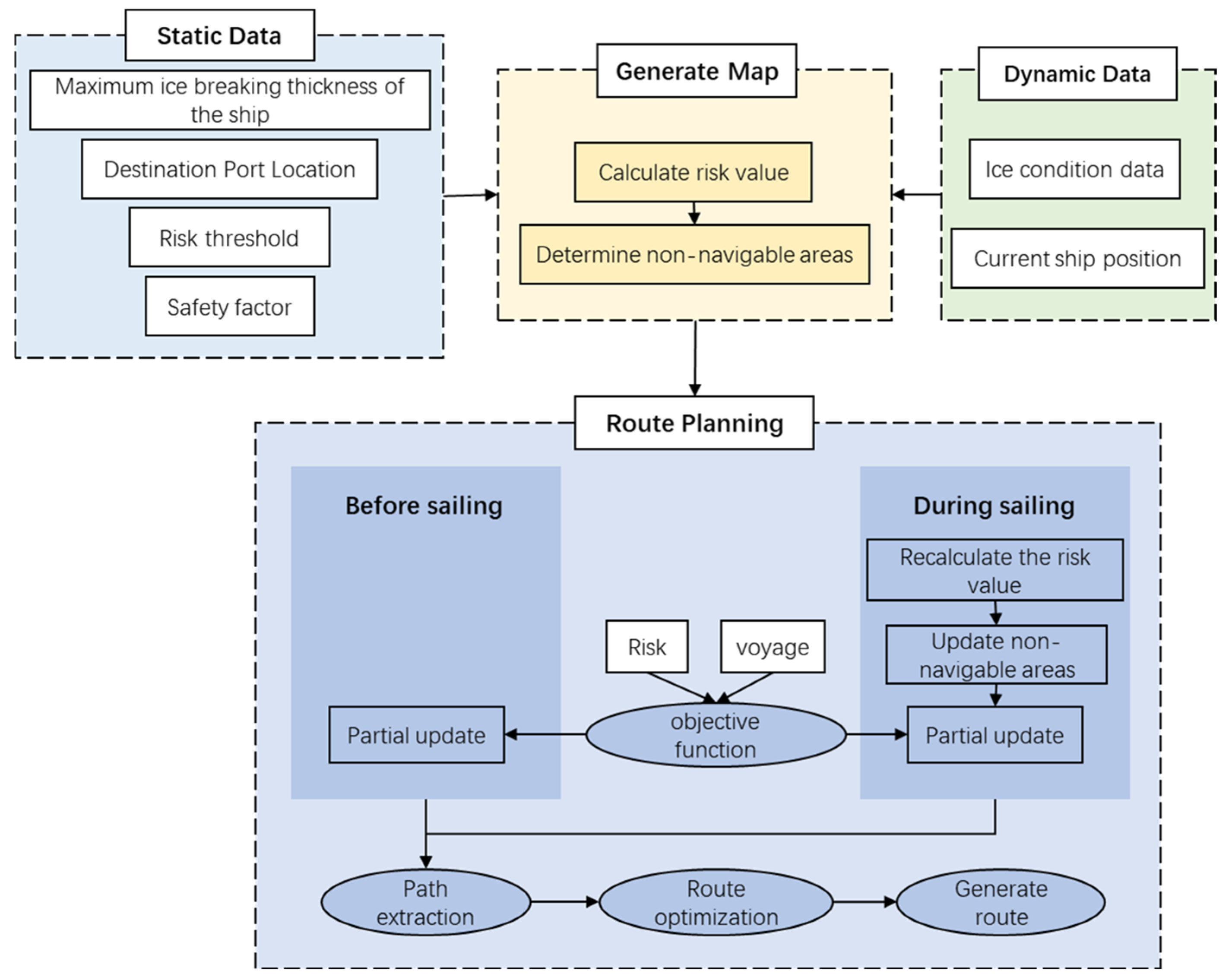
The ice routing model is designed to enable ships to effectively navigate through weak ice areas in ice-infested waters based on their icebreaking capabilities, thereby reducing risks and enhancing navigation efficiency. Existing studies have significantly matured risk prediction and effectiveness assessment in ice routing models [31,32]; hence, this paper will not investigate these aspects. The improved D* Lite algorithm employed in this study can adapt to the dynamic changes in ice conditions, facilitating real-time route planning during ship navigation while considering the ship’s icebreaking capabilities and pursuing multi-objective optimization. The specific concept of the ice routing model proposed in this paper is illustrated in Figure 6.

3.1. Determination of Non-Navigable Regions

When planning dynamic routes for ships in Arctic waters, identifying non-navigable areas is crucial. This involves considering geographical and geomorphological features, oceanic conditions, and meteorological factors. Non-navigable areas mainly include landmasses and islands, which can be identified through data tagging and filtering. Additionally, sea ice in Arctic waters significantly affects ship navigation. Areas with average sea ice thickness exceeding a ship’s maximum icebreaking capability risk hull damage and should be classified as non-navigable.

Currently, various ship classification societies have established ice classes based on ships’ navigation capabilities under diverse sea ice conditions. Among these, the ice class standards from the International Association of Classification Societies (IACS), the Russian Maritime Register of Shipping (RS), and the Finnish–Swedish Ice Class Rule (FSICR) are widely recognized and applied. Detailed classification criteria are provided in

Table 2. Comparison table of ice classifications by major classification societies.

IACS	RS	FSICR	Navigable Sea Conditions/Seasons
PC-1			Navigate in all polar waters throughout the year	All polar waters throughout the year
	Arc9
PC-2			Navigate beneath the multi-year ice cover throughout the year
	Arc8	data
PC-3		data	Navigate in the second-year sea ice area throughout the year
	Arc7	data
PC-4		data	Navigate throughout the year in areas of moderately thick first-year ice
	Arc6	data
PC-5		data	Navigate throughout the year in areas of relatively thin first-year ice
PC-6	Arc5	IA Super	In Arctic waters during summer	In the sub-Arctic waters during winter
PC-7	Arc4	IA
	Ice3	IB
	Ice2	IC
	Ice1	II

.

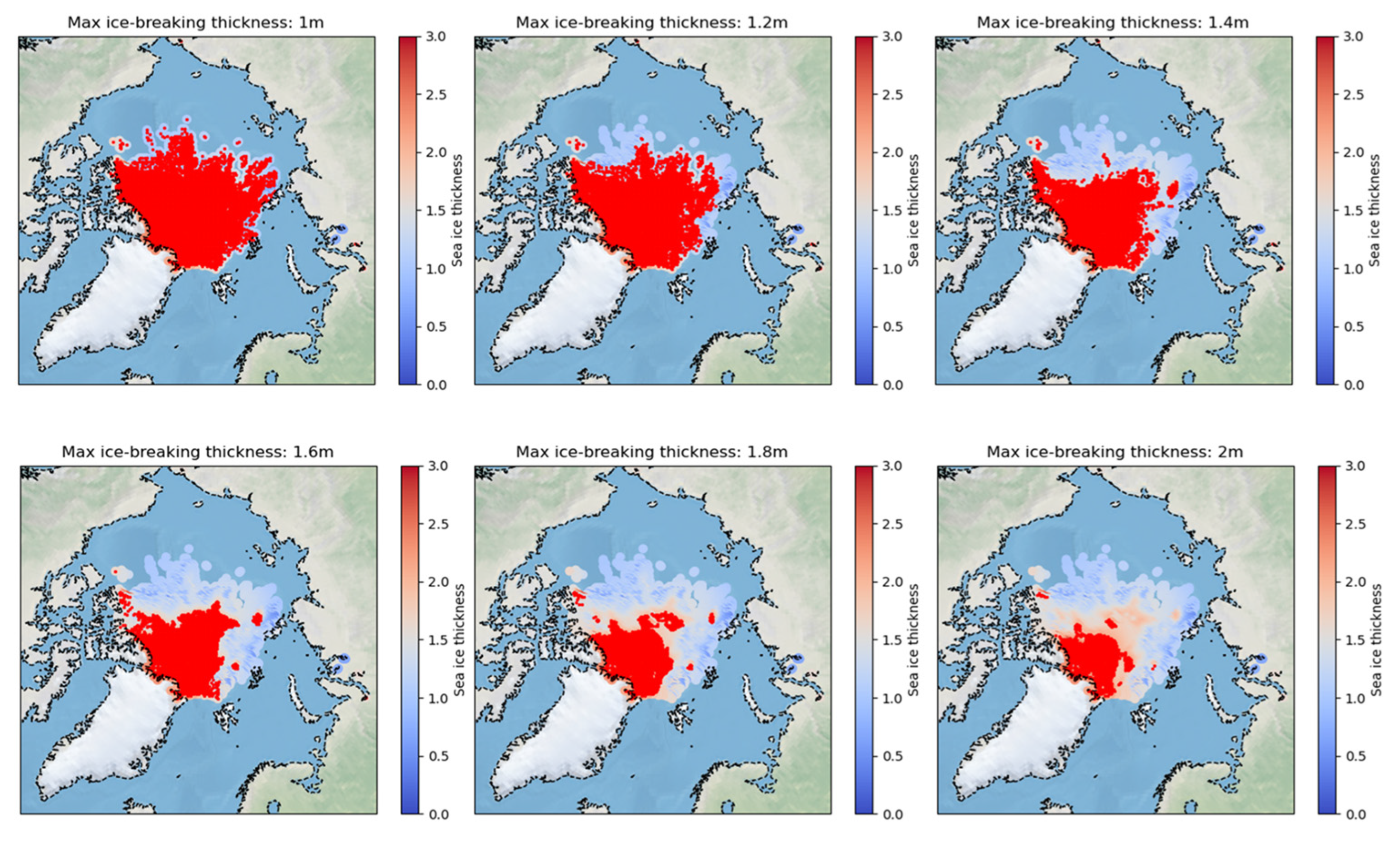
As shown in Table 2, the descriptions of navigable conditions provided by various ice class standards are not uniform, and there are no clear specifications for the maximum continuous ice-breaking thickness corresponding to different ice classes. Additionally, ice condition forecast data primarily provides sea ice thickness without specifying the ice type. To effectively use these forecasts and achieve precise route planning, this model uses the ship’s maximum continuous ice-breaking thickness as the metric for icebreaking capability, rather than the ship’s ice class. When the average sea ice thickness in a region exceeds the maximum continuous ice-breaking thickness of a ship, the area is classified as non-navigable. Figure 7 illustrates the navigable areas for ships with different icebreaking capabilities under the same ice conditions, with non-navigable areas marked in red. It demonstrates that ships with higher icebreaking capabilities encounter fewer non-navigable areas, thereby enjoying greater navigational freedom.

Additionally, the regional risk coefficient is one of the important indicators for determining non-navigable areas. Typically, the risk coefficient for a given area can be calculated by assessing various factors such as marine weather conditions, hydrological conditions, and changes in ice conditions [33]. If the risk coefficient for a specific area exceeds a predetermined threshold, it should be classified as a non-navigable area to prevent ships from encountering unexpected damage or distress. The calculation formula for the risk coefficient $r$ in this model is as follows:

$$r={\displaystyle \frac{h\times C}{Ic{e}_{max}}},$$

(10)

where $h$ represents the average ice thickness, $C$ denotes the ice density, and $Ic{e}_{max}$ refers to the ship’s maximum continuous ice-breaking thickness. This formula ensures that the navigation risk calculation results for all navigable areas fall between 0 and 1.

For the same ship, setting different predetermined risk thresholds will result in variations in its navigable area. Figure 8 illustrates the navigable areas for the same ship configured with different risk thresholds, with non-navigable areas marked in red. it can be concluded that the higher the set risk threshold, the fewer the number of non-navigable areas, thereby increasing the ship’s navigational freedom.

In summary, the non-navigable areas in this model encompass (1) continents or islands; (2) seas where the average sea ice thickness exceeds the ship’s maximum continuous ice-breaking thickness; and (3) seas with a regional risk coefficient higher than the pre-determined risk threshold for the voyage.

3.2. Establishing the Objective Function

Different types of ships, such as general merchant ships, research ships, and polar sightseeing ships, have varying emphases in route planning. The requirements for routes of the same ship can change when considering various factors such as cargo types and customer needs. Therefore, ship routes often need to be flexibly adjusted to plan routes that meet expectations.

Journey and risk are the two primary objectives in the multi-objective planning research of ship routes in icy regions [34]. In the model, both distance and risk are normalized values. Since the algorithm employs an eight-neighborhood movement, the formula for calculating the movement distance $d$ between adjacent nodes is as follows:

$$d={\displaystyle \frac{\sqrt{{\left(x_s-x_{s^{\prime }}\right)}^2+{\left(y_s-y_{s^{\prime }}\right)}^2}}{\sqrt{2}}},$$

(11)

where $x_s$ and $y_s$ represent the coordinates of point $s$, and $x_{s^{\prime }}$ and $y_{s^{\prime }}$ denote the coordinates of the adjacent node $s^{\prime }$. The distance $d$ calculated from the equation is either 1 or 0.707, and under normal circumstances, its value is higher than the risk value $r$. To achieve multi-objective planning, it is necessary to maximize the influence of the risk value $r$ on the movement cost $\mathrm{c}\mathrm{o}\mathrm{s}t$ of the adjacent nodes. Therefore, this model does not use weight calculations but instead introduces the risk coefficient; the formula for calculating the movement cost $cost$ in this model is as follows:

$$cost=\delta \cdot r+d,$$

(12)

where $\delta$ represents the safety coefficient. A higher $\delta$ value increases the influence of the risk value $r$ on the movement cost $\mathrm{c}\mathrm{o}\mathrm{s}t$ of adjacent nodes.

Consequently, the safety coefficient $\delta$ positively correlates with route safety; a higher $\delta$ prioritizes areas with lower average sea ice thickness or density as path nodes, enhancing overall safety. Theoretically, $\delta$ can range from 0 to ∞, with its effective range depending on the risk–distance relationship. Simulation experiments showed that, within the objective function framework, a safety coefficient of 3 yielded near-peak safety routes. Increasing $\delta$ beyond this did not significantly alter route planning outcomes, suggesting that a safety coefficient of 3 is sufficient to effectively ensure route safety, eliminating the need for further increases.

To assess the overall risk of a route, it is not sufficient to rely solely on the minimum or maximum risk values but should consider the average risk coefficient over the entire voyage. In this model, the calculation formula for the average risk $R$ of the entire voyage route is as follows:

$$R={\displaystyle \frac{\sum _{i=1}^n\left(r_i\times d_i\right)}{\sum _{i=1}^n{d}_i}},$$

(13)

where $r_i$ represents the risk value at the $i$-th node in the route. It is worth noting that the improved algorithm updates a lower number of nodes during route re-planning, indicating that the advantages of this ice routing model become more evident when the complexity of the objective function is higher.

4. Analysis of Simulation Cases

The case study area spans from 55° N to 90° N, with a grid matrix size of 448 × 304 and a grid resolution of 25 km × 25 km. The ice data used in this study are derived from CryoSat-2 of the European Space Agency.

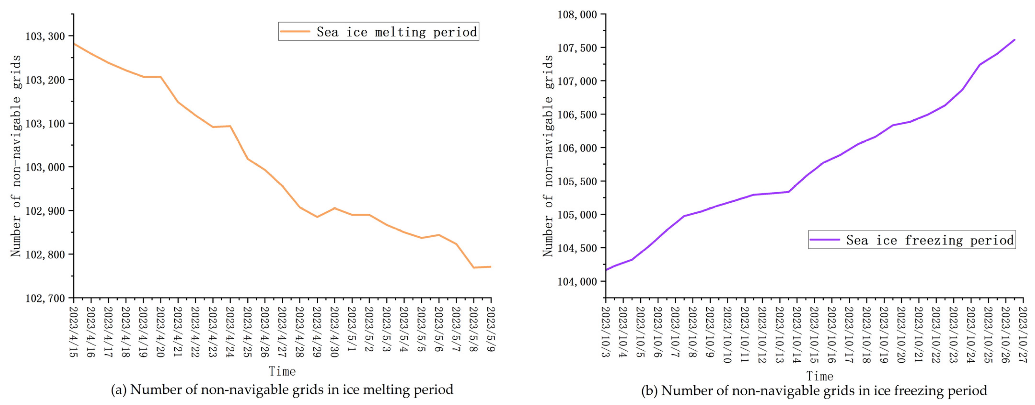
Given that the observations of sea ice thickness are not sufficiently accurate during rapidly changing months, and the ice data release platform did not provide data of average ice thickness from June to September, this study selects ice condition data from mid-April to mid-May and October as representatives for the break-up and freezing periods. As illustrated in Figure 9, during the specified periods, the variation in the number of non-navigable areas in the ice condition data used for the experiments aligns with expectations. To ensure that ships can navigate independently during these months, the maximum continuous icebreaking thickness for ships are at 2.8 m and 1.2 m, with a uniform risk threshold of 1. This study primarily aims to validate the practicality of the improved dynamic programming algorithm in Arctic waters, with a focus on assessing the efficiency and accuracy of the planning algorithm, while not considering factors such as varying speeds of ships in different ice conditions. Therefore, in the simulation experiments, the update distance for each ship position is constant, set at 8 unit grid distances, approximately equivalent to 432 nautical miles.

4.1. Freezing Period Simulation Planning

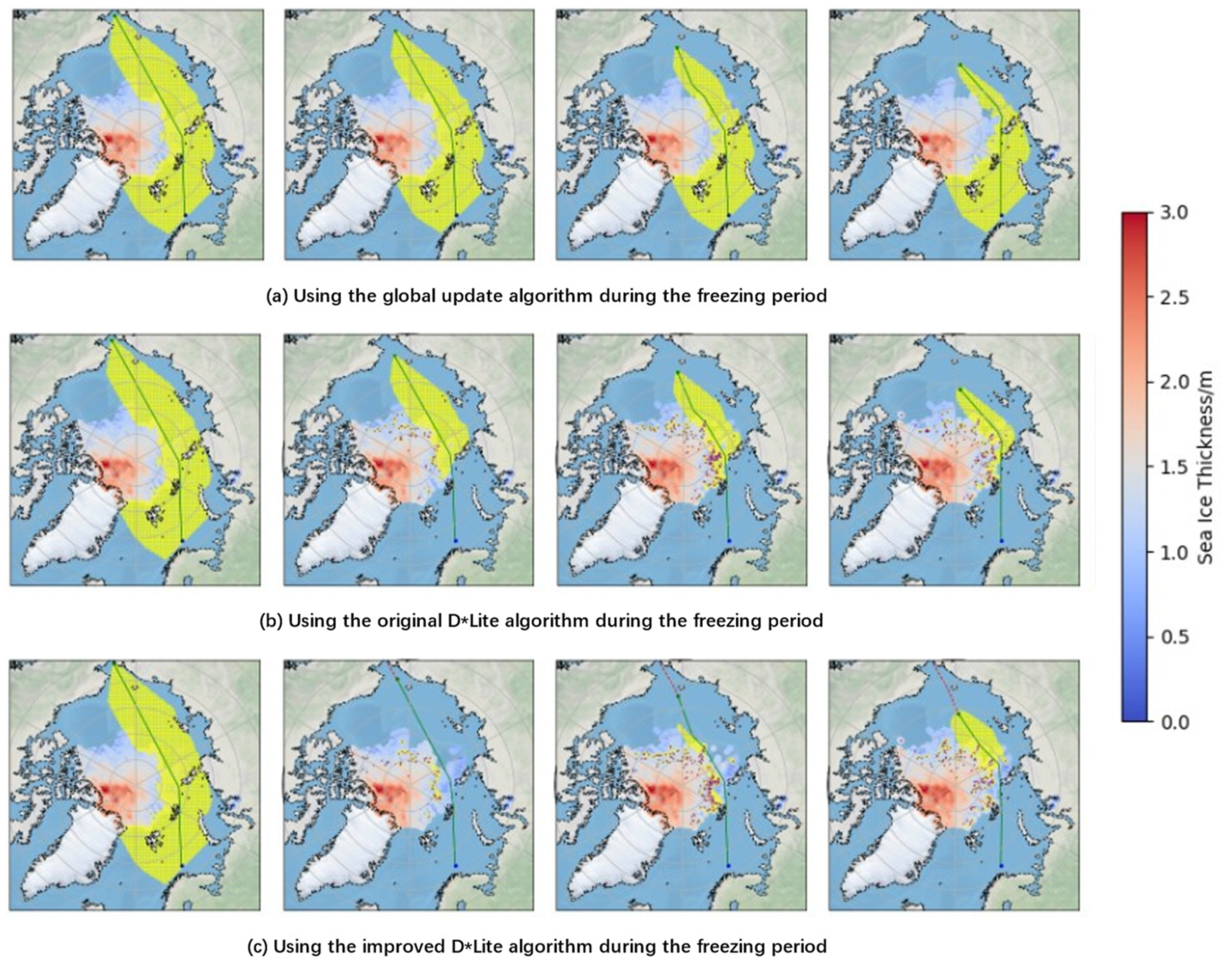
For the freezing period, the October 2023 dataset was used to validate the dynamic route planning capabilities of ships in ice-covered regions. To account for the significant increase in ice thickness, the maximum continuous ice-breaking thickness was set to 1.2 m, with a risk threshold of 1. Figure 10 illustrates the dynamic route planning processes of the global update algorithm, the original D* Lite algorithm, and the improved D* Lite algorithm during this period. Green markers indicate the current ship position, blue markers denote the target area, solid green lines represent the planned route based on current position and updated ice conditions, red dashed lines show the historical trajectory, purple grid points mark areas with navigability changes, and yellow areas highlight locally updated regions.

The simulation results effectively demonstrate the adaptability and efficiency of the dynamic route planning algorithm based on the latest ship position. In the increasingly harsh marine conditions of the freezing period, this algorithm can flexibly adjust the route to effectively evade newly introduced non-navigable areas and reduce navigation risk by steering towards lower latitudes. The final voyage distance increased from the initially planned 2460 nautical miles to 2558 nautical miles. This trend not only aligns with the expected outcomes of the experiment but also reflects the strategies commonly employed by ships in actual navigation when dealing with adverse ice conditions.

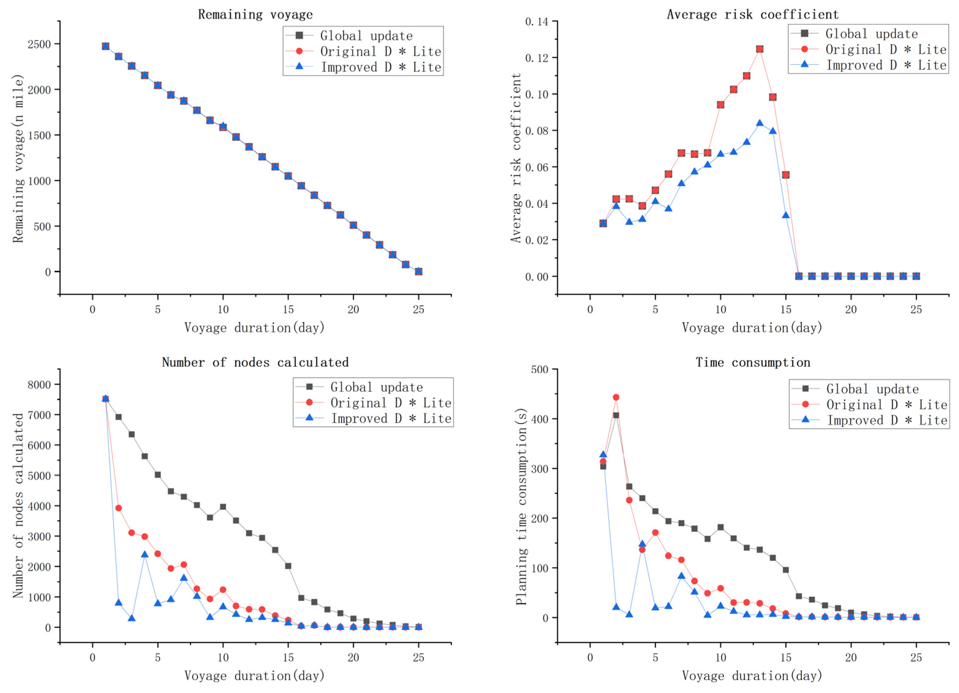
To further validate the effectiveness and planning efficiency of the improved algorithm for route planning during the freezing period, this study conducted an in-depth comparative analysis. Figure 11 clearly presents detailed data comparisons between the planning results of the improved D* Lite algorithm, the original D* Lite algorithm, and the global re-planning results across 26 route updates over the entire journey, all under the same new ship position and latest ice condition data. The figure records the number of updated nodes, planning time, remaining voyage distance, and the average risk coefficient of the remaining voyage during each dynamic route planning process.

The comparison of remaining voyage distance and risk coefficients is used to assess the quality of the planned route. The route obtained through global re-planning is optimal under the same heuristic function; thus, the closer these two indicators of the improved algorithm are to those of the global re-planning, the higher the effectiveness of its route. The comparison of planning time and the number of updated nodes is used to evaluate the operational efficiency of the algorithm. The improved algorithm significantly reduces these two indicators by modifying the node cost update rules and decreasing the update of irrelevant nodes. The figure shows that the voyage distance of the new routes planned by the improved D* Lite algorithm is generally consistent with those of the other two algorithms, with a slightly lower overall risk coefficient, as well as the lowest planning time and number of updated nodes among the three algorithms. This reduction is attributed to the improved algorithm’s ability to selectively update only relevant nodes by identifying critical areas in the map. According to

Table 3. Comparison table of route data using different algorithms during the freezing period.

Algorithms	Total Voyage Distance (n mile)	Average Risk Coefficient	Planning Time Consumption (s)	Number of Nodes Calculated
Global update	2561.408	0.076	3392	72,835
Original D* Lite	2561.408	0.076	1720	28,351
Improved D* Lite	2558.747	0.076	924	18,468

, the routes planned by the original D* Lite algorithm and the global re-planning algorithm are identical. The voyage and risk errors of the improved D* Lite algorithm compared to the original D* Lite algorithm and the global re-planning algorithm were 0.1% and 0.07%, respectively. The number of updated nodes decreased by 34.9% and 74.6%, and the planning time was reduced by 46.2% and 72.7%.

4.2. Melting Period Simulation Planning

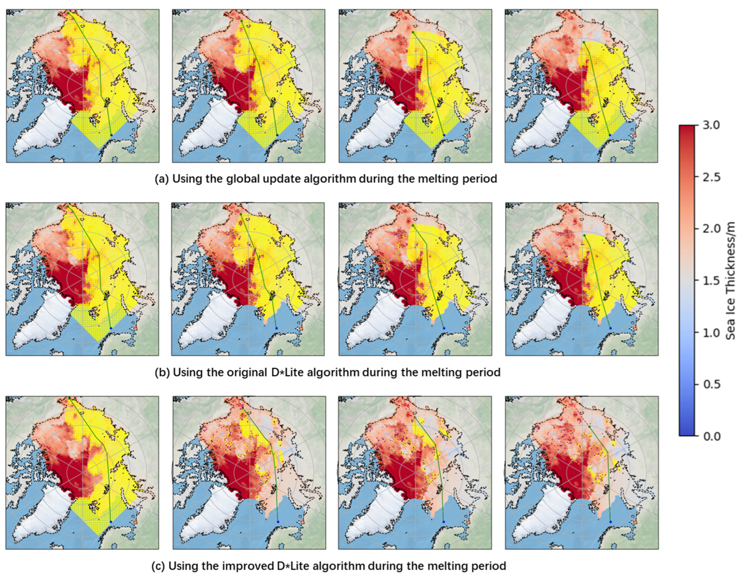
For the Melting period, a dataset covering mid-April to mid-May 2023 is selected in this paper for simulation validation to examine the ice routing models during this period. Despite the gradual decrease in ice thickness, the overall ice conditions remained severe [32]. To ensure that the ships could sail independently through ice during the experiment, the maximum continuous ice-breaking thickness was set at 2.8 m, with the highest risk threshold set at 1. Figure 12 provides a detailed illustration of the process of global update algorithm, the original D* Lite algorithm, and the improved D* Lite algorithm in performing dynamic ship route planning during the melting period. The green markers represent the current ship position, while the blue markers denote the target area. The solid green line indicates the subsequent route planned based on the current ship position and the latest ice condition data, the red dashed line represents the historical navigation trajectory, the purple grid points indicate areas where navigability has changed, and the yellow areas denote the locally updated regions.

The simulation results indicate that the dynamic route planning algorithm based on the latest ship position information proposed in this study demonstrated outstanding performance during the melting period. This algorithm not only adapts to the improving ice conditions but also fully utilizes newly available navigable areas to plan safer and more efficient routes for ships. As the ice conditions continue to improve, the newly planned routes gradually extend to higher latitudes. This strategic adjustment not only aligns with the expected outcomes of the experiment but also accurately reflects the flexible adjustments in navigation strategies that ships typically employ during the melting period.

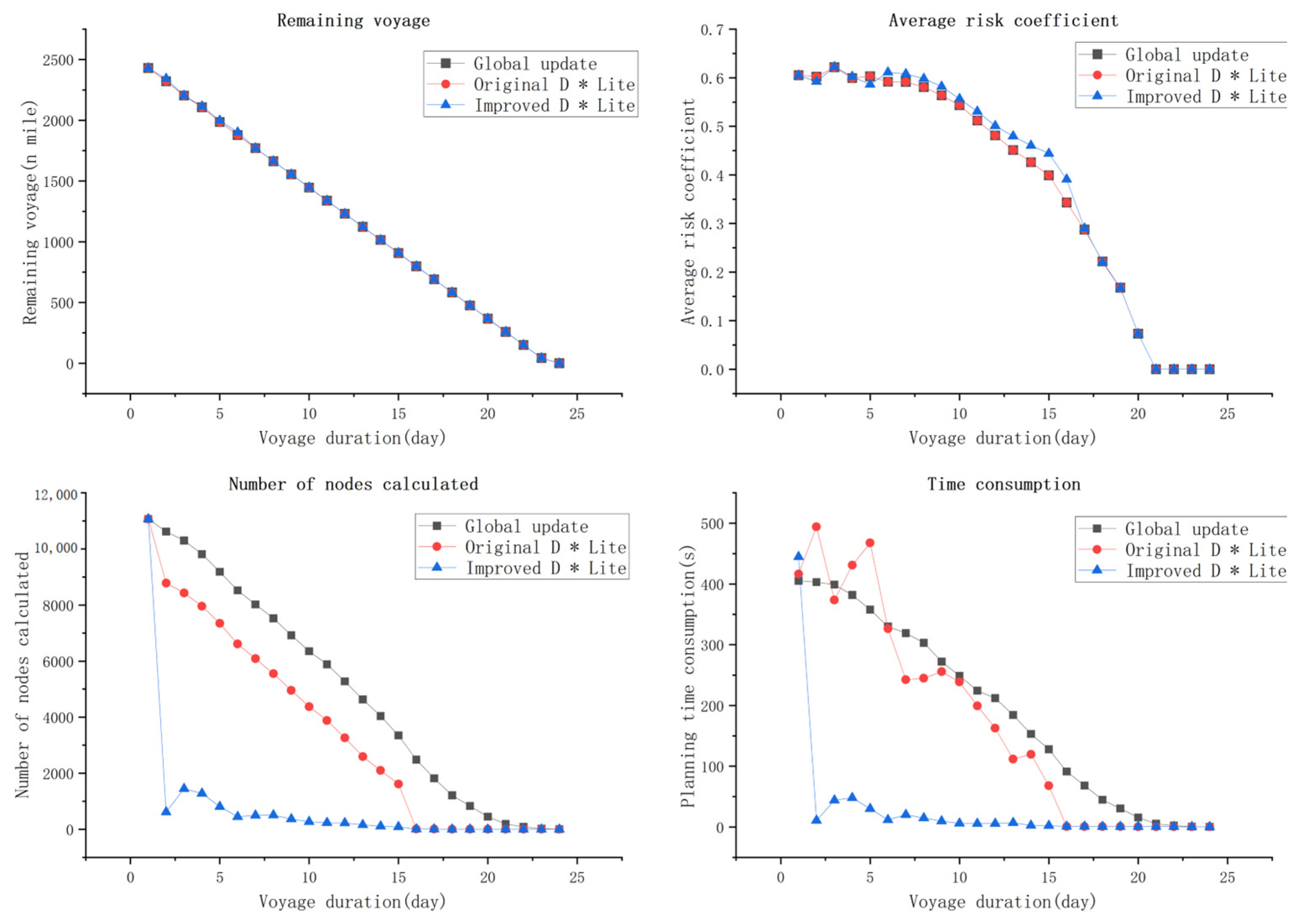
To further validate the effectiveness and planning efficiency of the dynamic route planning algorithm during the melting period, this study conducted a comparative analysis of route data similar to that used in the freezing period. Figure 13 provides a detailed comparison of the planning results obtained using the improved D* Lite algorithm, the original D* Lite algorithm, and the global re-planning approach across 24 route updates over the entire journey, all based on the new ship position and the latest ice condition data.

The routes planned by the improved algorithm are comparable to those of the other two algorithms in terms of remaining voyage distance and risk coefficient, indicating its continued effectiveness during the ice-melting period. Compared to the freezing period, the algorithm exhibits more significant reductions in planning time and the number of updated nodes during the ice-melting period. This is attributed to the wider ice coverage and more available ice condition data during the ice-melting period, which allows the algorithm’s modifications to the node cost update rules to be more advantageous. According to

Table 4. Comparison table of route data using different algorithms during the melting period.

Algorithms	Total Voyage Distance (n mile)	Average Risk Coefficient	Planning Time Consumption (s)	Number of Nodes Calculated
Global update	2418.146	0.615	4770	114,929
Original D* Lite	2418.146	0.615	4409	82,210
Improved D* Lite	2419.087	0.615	632	16,864

, the voyage distance and risk errors for the improved D* Lite algorithm, compared to the original D* Lite and global re-planning algorithms, were 0.07% and 0.07%, respectively. Additionally, the number of updated nodes decreased by 79.5% and 85.3%, while the planning time was reduced by 85.7% and 86.7%, respectively.

Figure 14 illustrates the complete dynamic routes planned by the three algorithms during the melting period and the freezing period. As can be seen from the figure, three algorithms exhibit high consistency during the freezing period and the melting period, which verifies the effectiveness of the dynamically planned routes. Additionally, the data comparison on planning time and the number of updated nodes clearly demonstrates significant improvement in the planning efficiency of the improved algorithm, with a strong correlation observed between the planning time and the number of updated nodes. As the ship progressively approaches the target sea area, the proportion of nodes that significantly impact the route results among all change nodes gradually decreases, indirectly leading to further reductions in planning time and the number of updated nodes.

4.3. Verification of Model Effectiveness

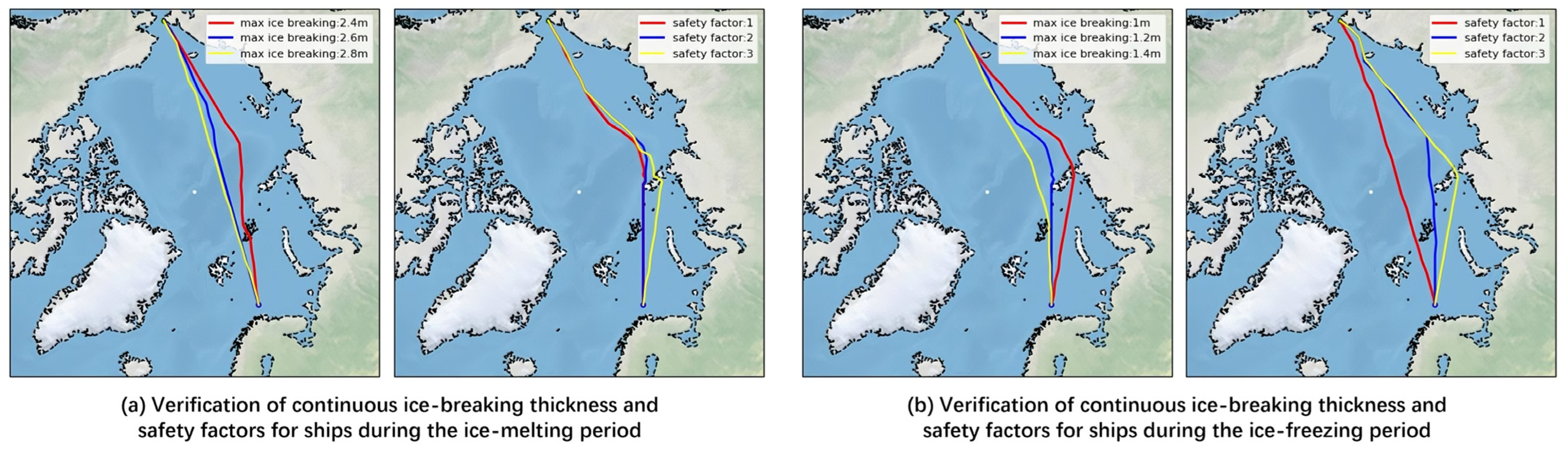
To further verify the validity of the model, a series of simulation analyses were conducted on its parameters by setting different continuous ice-breaking thicknesses and safety coefficients for the ship, in order to validate the effectiveness of these various parameters. Figure 15 separately displays the impact of the ship’s continuous ice-breaking thickness and safety coefficient on the model under different ice conditions.

A comparative analysis reveals a significant relationship between the maximum continuous ice-breaking thickness and the route planning results under the simulated ice condition data: As shown in

Table 5. Comparison table of route data planned by different parameters.

Period	Maximum Continuous Icebreaking Thickness (m)	Safety Coefficient	Total Voyage Distance (n mile)	Average Risk Coefficient
Freezing period	1	1	2654.492	0.002
	1.2	1	2558.747	0.076
	1.4	1	2459.904	0.113
	1.2	2	2576.925	0.070
	1.2	3	2645.540	0.039
Melting period	2.4	1	2480.926	0.625
	2.6	1	2428.497	0.631
	2.8	1	2419.087	0.615
	2.8	2	2550.582	0.510
	2.8	3	2644.126	0.468

, as the maximum continuous ice-breaking thickness increases, the total voyage distance of the complete route obtained from the model’s dynamic planning decreases accordingly, while the average risk coefficient exhibits an upward trend. Additionally, variations in the safety coefficients also have a significant impact on the route planning results: a higher safety coefficient corresponds to a longer total voyage length of the complete route obtained from the model’s dynamic planning, while the average risk coefficient decreases. Furthermore, due to the harsher ice conditions experienced during the ice melting period (April–May) compared to the freezing period (October) in the simulation, the overall average risk coefficient during the ice melting period is higher than that in the freezing period. This result meets the expectations and further validates the effectiveness and practicality of this model.

In summary, the results obtained from the improved dynamic programming algorithm demonstrate good validity and efficiency. The errors in voyage distance and average risk coefficient during both the freezing and melting periods are less than 0.1%, and the planning efficiency has improved by 35% and over 85%, respectively, compared to the previous version of the algorithm. In addition, this algorithm can generate corresponding optimal routes for ships with different ice-breaking capabilities. During both the freezing and melting periods, there are significant differences in the routes planned for ships with varying ice-breaking capabilities; specifically, ships with stronger ice-breaking abilities have routes that are closer to the central navigation channel, resulting in shorter voyage distances. Also, the improved dynamic programming algorithm is capable of planning routes with different safety levels for the same ship, catering to the needs of various voyages. During both the freezing and melting periods, for the same ship, a higher safety coefficient results in a longer voyage distance, while the average risk coefficient tends to be relatively lower.

5. Discussion

In this study, the POLARIS (Polar Operational Limit Assessment Risk Index System) released by the International Maritime Organization (IMO) was not used to calculate navigation risk, mainly due to two reasons. First, the POLARIS method calculates risk based on ice types rather than ice thickness, which does not match the format of ice condition data released by mainstream platforms. Second, the POLARIS method calculates risk based on the ship’s ice class rather than its maximum continuous ice-breaking thickness, resulting in an error margin when determining non-navigable areas, which may lead to ice bound or ship damage.

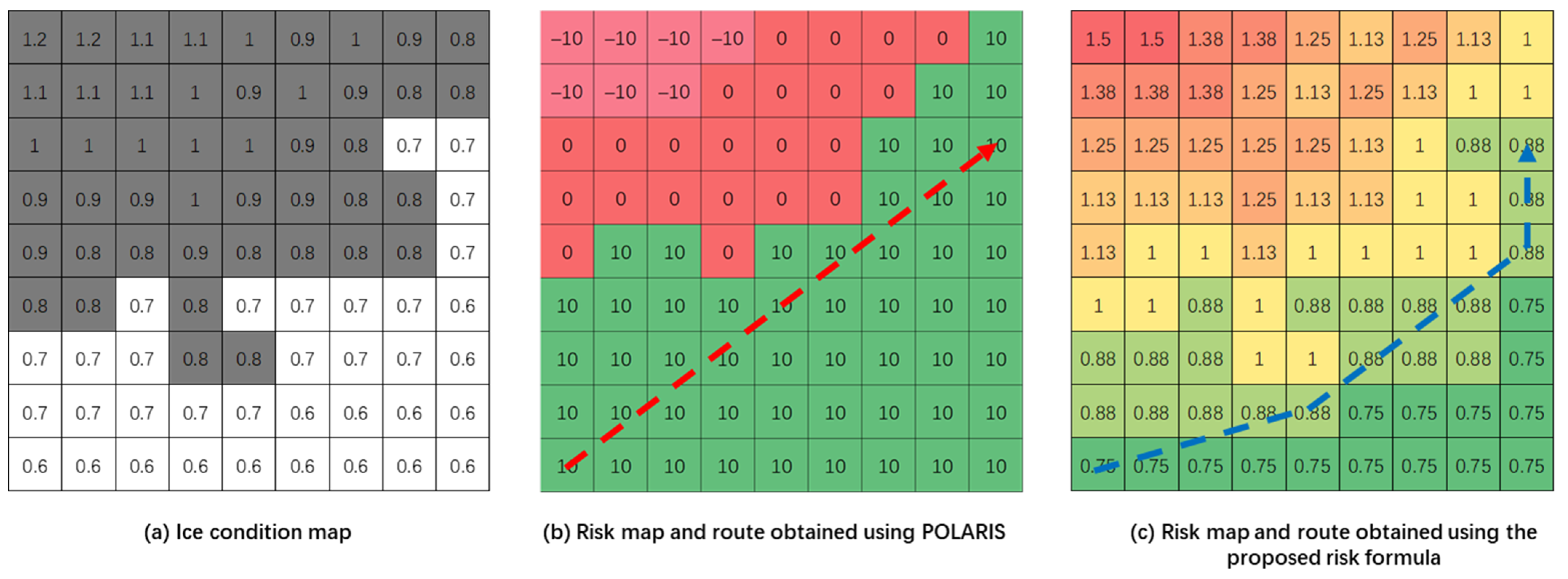
To address this issue, the risk calculation proposed in this study adopts average ice thickness and ice density as ice condition indicators, and uses the continuous maximum icebreaking thickness of the vessel as the measure of icebreaking capability, rather than the general classification based on ship ice class. This approach enhances the accuracy of risk calculations. To better illustrate the differences between the proposed risk calculation method and the POLARIS risk calculation method, the shortest routes were planned using both approaches on the same ice condition map. As shown in Figure 16, the different colors of the grid represent different risk coefficients, and the corresponding risk coefficients are annotated within the grid. we can observe the following assuming a ship with a maximum continuous icebreaking thickness of 0.8 m, corresponding to a PC-6 ice class vessel: Subplot (a) provides a simulated ice condition map, where the values within the grid cells represent average ice thickness, and the ice concentration is uniformly set to 100%. Gray grid cells indicate non-navigable areas. Subplot (b) shows the route planned using the POLARIS risk calculation method, with the grid values representing the RIO (Risk Index Outcome) defined by POLARIS, categorized into three levels of risk, where a lower RIO value indicates higher risk. Subplot (c) illustrates the route planned using the risk calculation method proposed in this study, with the grid values representing the calculated risk value $r$, where $r$ ≥ 1 indicates non-navigable areas, and a lower $r$ value indicates higher risk. It can be observed that the route planned using the POLARIS risk calculation method crosses some non-navigable areas, while the route planned using the proposed method avoids all non-navigable areas. Furthermore, the proposed method provides a more detailed stratification of risk, which facilitates refined route planning.

Furthermore, the uncertainty in ice condition forecast data and factors such as the movement of floating ice may render the ship’s current route ineffective, or even lead to routes passing through unnavigable areas. To address this issue, local obstacle avoidance algorithms need to be introduced to dynamically adjust the routes between adjacent paths. Therefore, in future work, based on the existing research, the improved algorithm will be applied to local dynamic obstacle avoidance, maximizing the utilization of global planning computing data and effectively combining it with global dynamic route planning to achieve real-time dynamic route planning for ships in Arctic waters.

6. Conclusions

This paper proposes an improved D* Lite algorithm to adapt to dynamic ice routing planning for ships in Arctic waters. Compared with other existing methods, this algorithm focuses on addressing the planning efficiency issue of dynamic programming algorithms in Arctic waters. It achieves efficiency improvements primarily by modifying the node cost update rules, rather than complicating the heuristic function, thereby enhancing efficiency from the underlying logic. To address the issue of excessively high route update costs associated with the original D* Lite algorithm in Arctic waters, the update rules for node cost values were first adjusted. Specifically, only the areas where navigability changes between the ship’s current position and the target region are considered as key nodes, flexibly adopting cost value update methods according to the characteristics of those changes. Additionally, to resolve the path extraction issues arising from the new update rules, new path extraction rules were formulated. Finally, by incorporating a path optimization algorithm, it is ensured that the ice routing closely approximates the optimal path, given the correct extraction of key path nodes.

The feasibility of the improved algorithm under varying ice condition changes and the effectiveness of its planned routes were validated using examples from the freezing and melting periods. Simulation results indicate that the model’s planned routes have an error of less than 0.1% compared to the optimal routes. Planning efficiency during the freezing and melting periods increased by 35% and over 85%.It indicates that the improvement in planning efficiency is directly proportional to the completeness of ice condition data within the planning area. To further assess the practicality of the model, simulations were conducted for different months under various scenarios of maximum continuous ice-breaking thicknesses and safety coefficients for ships, with the aim of planning corresponding ice routings and comparing the differences in those routings against actual conditions. A comparative analysis of the route data indicates that the ice navigation route planning model can efficiently provide optimal routes tailored to the safety needs of ships with varying ice-breaking capabilities.

References

- Koçak, S.T.; Yercan, F. Comparative cost-effectiveness analysis of Arctic and international shipping routes: A Fuzzy Analytic Hierarchy Process. Transp. Policy 2021, 114, 147–164. [Google Scholar] [CrossRef]
- Guo, J.; Guo, S.; Lv, J. Potential spatial effects of opening Arctic shipping routes on the shipping network of ports between China and Europe. Mar. Policy 2022, 136, 104885. [Google Scholar] [CrossRef]
- Afenyo, M.; Khan, F.; Veitch, B.; Yang, M. Arctic shipping accident scenario analysis using Bayesian Network approach. Ocean Eng. 2017, 133, 224–230. [Google Scholar] [CrossRef]
- Lin, B.; Zheng, M.; Chu, X.; Mao, W.; Zhang, D.; Zhang, M. An overview of scholarly literature on navigation hazards in Arctic shipping routes. Environ. Sci. Pollut. Res. Int. 2024, 31, 40419–40435. [Google Scholar] [CrossRef]
- Sahin, B.; Kum, S. Risk assessment of Arctic navigation by using improved fuzzy-AHP approach. Int. J. Marit. Eng. 2015, 157, A-241–A-250. [Google Scholar] [CrossRef]
- Chen, X.; Liu, S.; Liu, R.W.; Wu, H.; Han, B.; Zhao, J. Quantifying Arctic oil spilling event risk by integrating an analytic network process and a fuzzy comprehensive evaluation model. Ocean Coast. Manag. 2022, 228, 106326. [Google Scholar] [CrossRef]
- Wang, C.; Ding, M.; Yang, Y.; Wei, T.; Dou, T. Risk Assessment of Ship Navigation in the Northwest Passage: Historical and Projection. Sustainability 2022, 14, 5591. [Google Scholar] [CrossRef]
- Zhang, C.; Zhang, D.; Zhang, M.; Lang, X.; Mao, W. An integrated risk assessment model for safe Arctic navigation. Transp. Res. Part A Policy Pract. 2020, 142, 101–114. [Google Scholar] [CrossRef]
- Li, Z.; Yao, C.; Zhu, X.; Gao, G.; Hu, S. A decision support model for ship navigation in Arctic waters based on dynamic risk assessment. Ocean Eng. 2022, 244, 110427. [Google Scholar] [CrossRef]
- Brown, R.C. An Experimental Investigation of Ship Manoeuvrability in Pack Ice. Ph.D. Thesis, Memorial University of Newfoundland, St. John’s, NL, Canada, 2002. [Google Scholar]
- Yang, B.; Zhang, G.; Huang, Z.; Sun, Z.; Zong, Z. Numerical simulation of the ice resistance in pack ice conditions. Int. J. Comput. Methods 2020, 17, 1844005. [Google Scholar] [CrossRef]
- Kim, J.-H.; Kim, Y.; Lu, W. Prediction of ice resistance for ice-going ships in level ice using artificial neural network technique. Ocean Eng. 2020, 217, 108031. [Google Scholar] [CrossRef]
- Kotovirta, V.; Jalonen, R.; Axell, L.; Riska, K.; Berglund, R. A system for route optimization in ice-covered waters. Cold Reg. Sci. Technol. 2009, 55, 52–62. [Google Scholar] [CrossRef]
- Nam, J.-H.; Park, I.; Lee, H.J.; Kwon, M.O.; Choi, K.; Seo, Y.-K. Simulation of optimal arctic routes using a numerical sea ice model based on an ice-coupled ocean circulation method. Int. J. Nav. Archit. Ocean Eng. 2013, 5, 210–226. [Google Scholar] [CrossRef]
- Choi, M.; Chung, H.; Yamaguchi, H.; Nagakawa, K. Arctic sea route path planning based on an uncertain ice prediction model. Cold Reg. Sci. Technol. 2015, 109, 61–69. [Google Scholar] [CrossRef]
- Zhang, C.; Zhang, D.; Zhang, M.; Mao, W. Data-driven ship energy efficiency analysis and optimization model for route planning in ice-covered Arctic waters. Ocean Eng. 2019, 186, 106071. [Google Scholar] [CrossRef]
- Topaj, A.G.; Tarovik, O.V.; Bakharev, A.A.; Kondratenko, A.A. Optimal ice routing of a ship with icebreaker assistance. Appl. Ocean Res. 2019, 86, 177–187. [Google Scholar] [CrossRef]
- Lehtola, V.; Montewka, J.; Goerlandt, F.; Guinness, R.; Lensu, M. Finding safe and efficient shipping routes in ice-covered waters: A framework and a model. Cold Reg. Sci. Technol. 2019, 165, 102795. [Google Scholar] [CrossRef]
- Lee, H.-W.; Roh, M.-I.; Kim, K.-S. Ship route planning in Arctic Ocean based on POLARIS. Ocean Eng. 2021, 234, 109297. [Google Scholar] [CrossRef]
- Zhang, C.; Zhang, D.; Zhang, M.; Zhang, J.; Mao, W. A three-dimensional ant colony algorithm for multi-objective ice routing of a ship in the Arctic area. Ocean Eng. 2022, 266, 113241. [Google Scholar] [CrossRef]
- Shu, Y.; Zhu, Y.; Xu, F.; Gan, L.; Lee, P.T.-W.; Yin, J.; Chen, J. Path planning for ships assisted by the icebreaker in ice-covered waters in the Northern Sea Route based on optimal control. Ocean Eng. 2023, 267, 113182. [Google Scholar] [CrossRef]
- Li, B.; Gong, J.; Zhao, X.; Cheng, X. Research on ship navigation strategy in dynamic sea ice environments based on flexibility velocity obstacles algorithm. Ocean Eng. 2024, 311, 118843. [Google Scholar] [CrossRef]
- Liu, Q.; Wang, Y.; Zhang, R.; Yan, H.; Xu, J.; Guo, Y. Arctic weather routing: A review of ship performance models and ice routing algorithms. Front. Mar. Sci. 2023, 10, 1190164. [Google Scholar] [CrossRef]
- Sandven, S.; Spreen, G.; Heygster, G.; Girard-Ardhuin, F.; Farrell, S.L.; Dierking, W.; Allard, R.A. Sea Ice Remote Sensing—Recent Developments in Methods and Climate Data Sets. Surv. Geophys. 2023, 44, 1653–1689. [Google Scholar] [CrossRef]
- Zhong, W.; Jiang, M.; Xu, K.; Jia, Y. Arctic Sea Ice Lead Detection from Chinese HY-2B Radar Altimeter Data. Remote Sens. 2023, 15, 516. [Google Scholar] [CrossRef]
- Koenig, S.; Likhachev, M. D* lite. In Proceedings of the Eighteenth National Conference on Artificial Intelligence, Edmonton, AB, Canada, 30 July–1 August 2002; pp. 476–483. [Google Scholar]
- Yoon, S.; Shim, D.H. SLPA*: Shape-Aware Lifelong Planning A* for Differential Wheeled Vehicles. IEEE Trans. Intell. Transp. Syst. 2014, 16, 730–740. [Google Scholar] [CrossRef]
- Stentz, A.; Mellon, I.C. Optimal and efficient path planning for unknown and dynamic environments. Int. J. Robot. Autom. 1995, 10, 89–100. [Google Scholar]
- Zhang, Q.; Luo, H.; Min, C.; Xiu, Y.; Shi, Q.; Yang, Q. Evaluation of Arctic Sea Ice Thickness from a Parameter-Optimized Arctic Sea Ice–Ocean Model. Remote Sens. 2023, 15, 2537. [Google Scholar] [CrossRef]
- Sun, X.; Lv, T.; Sun, Q.; Ding, Z.; Shen, H.; Gao, Y.; He, Y.; Fu, M.; Li, C. Analysis of Spatiotemporal Variations and Influencing Factors of Sea Ice Extent in the Arctic and Antarctic. Remote Sens. 2023, 15, 5563. [Google Scholar] [CrossRef]
- Feng, J.; Li, J.; Zhong, W.; Wu, J.; Li, Z.; Kong, L.; Guo, L. Daily-Scale Prediction of Arctic Sea Ice Concentration Based on Recurrent Neural Network Models. J. Mar. Sci. Eng. 2023, 11, 2319. [Google Scholar] [CrossRef]
- Wu, D.; Tian, W.; Lang, X.; Mao, W.; Zhang, J. Statistical Modeling of Arctic Sea Ice Concentrations for Northern Sea Route Shipping. Appl. Sci. 2023, 13, 4374. [Google Scholar] [CrossRef]
- An, L.; Ma, L.; Wang, H.; Zhang, H.-Y.; Li, Z.-H. Research on navigation risk of the Arctic Northeast Passage based on POLARIS. J. Navig. 2022, 75, 455–475. [Google Scholar] [CrossRef]
- Zhao, W.; Wang, H.; Geng, J.; Hu, W.; Zhang, Z.; Zhang, G. Multi-Objective Weather Routing Algorithm for Ships Based on Hybrid Particle Swarm Optimization. J. Ocean Univ. China 2022, 21, 28–38. [Google Scholar] [CrossRef]
Figure 1.
Comparison of path planning algorithms for graph search path.
Figure 2.
Schematic diagram of the updated area before and after algorithm improvement.
Figure 3.
Schematic diagram of path extraction before and after algorithm improvement.
Figure 4.
Schematic diagram of path cost calculation.
Figure 5.
Path optimization rendering.
Figure 6.
Concepts of the proposed ice routing model.
Figure 7.
Non-navigable regions for ships with different icebreaking capabilities.
Figure 8.
Non-navigable regions for the same ship at different risk thresholds.
Figure 9.
Trend chart of non-navigable grid quantity changes.
Figure 10.
Comparison of route planning using different algorithms during the freezing period.
Figure 11.
Data chart of route planning using different algorithms during the freezing period.
Figure 12.
Comparison of route planning using different algorithms during the melting period.
Figure 13.
Data chart of route planning using different algorithms during the melting period.
Figure 14.
Comparison chart of route planning using different algorithms.
Figure 15.
Comparison chart of routes planned with different parameters.
Figure 16.
Comparison chart of the risk calculation formula proposed in this paper and the POLARIS risk calculation method.