
Analyzing Archive Transit Multibeam Data for Nodule Occurrences

 , ,
, ,
Abstract
1. Introduction
2. Observations
2.1. Transit Observations and Geological Setting
2.2. Environmental Parameters Suitable for Nodule Formation
2.3. Transit Areas Aligning with Prospective Nodule Characteristics
3. Research Objectives
4. Materials and Methods
4.1. 8-Bit Graphic Paper Chart Analysis
4.2. Comparing 8-Bit Graphic Paper Chart with Digital Backscatter Products
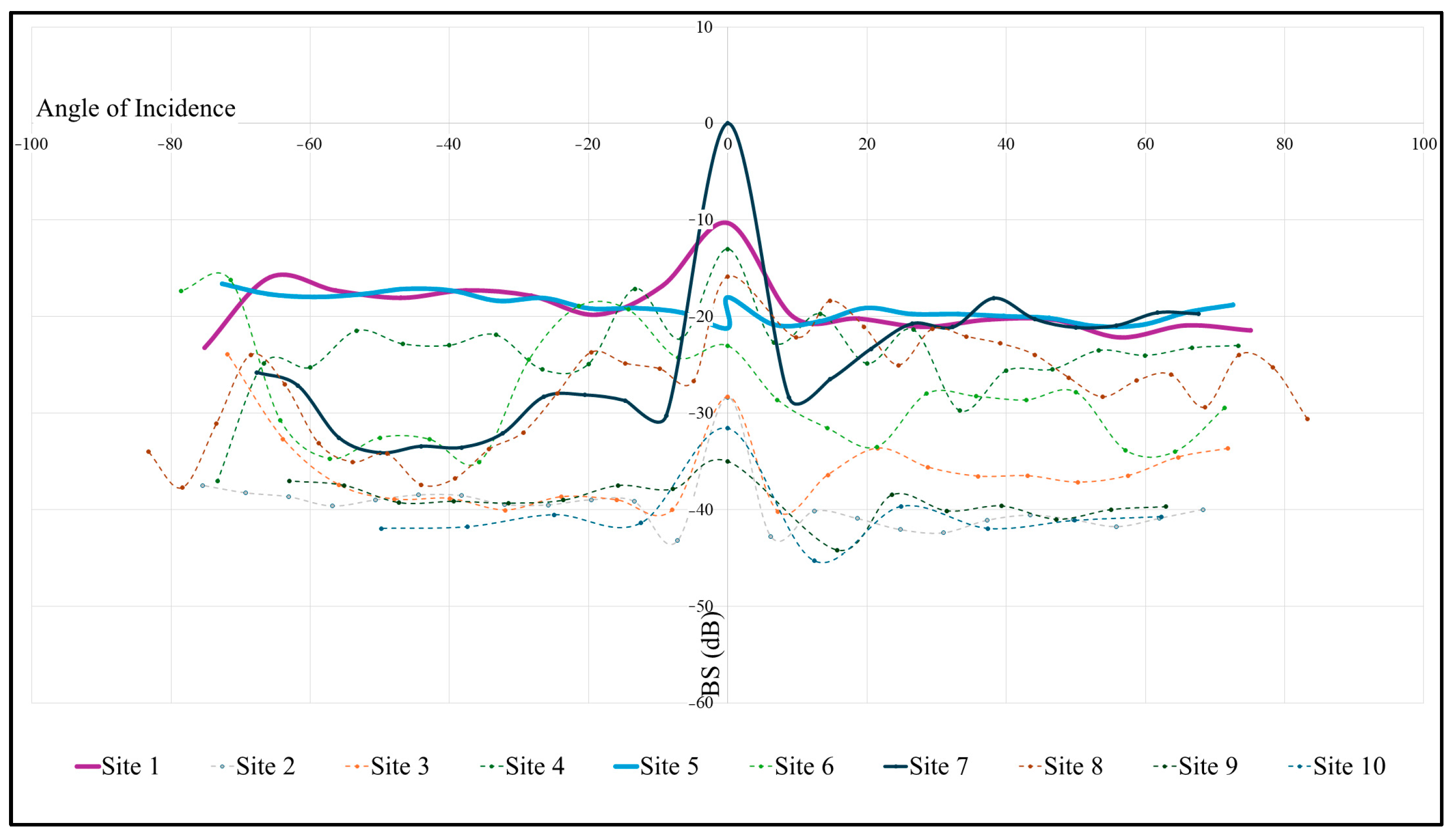
4.3. Comparing Angular Response
5. Results
6. Discussion
7. Conclusions
Supplementary Materials
Author Contributions
Funding
Institutional Review Board Statement
Informed Consent Statement
Data Availability Statement
Acknowledgments
Conflicts of Interest
References
- Hein, J.R.; Koschinsky, A. Deep-Ocean Ferromanganese Crusts and Nodules. In Treatise on Geochemistry; Elsevier: Amsterdam, The Netherlands, 2014; Volume 13, pp. 273–291. [Google Scholar]
- Kodagali, V.N.; Chakraborty, B. Multibeam Echosounder Pseudo Sidescan Images as a Tool for Manganese Nodule Exploration. In Proceedings of the ISOPE Ocean Mining and Gas Hydrates Symposium, Goa, India, 8–10 November 1999; pp. 97–104. [Google Scholar]
- Kuhn, T.; Wegorzewski, A.; Rühlemann, C.; Vink, A. Composition, Formation, and Occurrence of Polymetallic Nodules. In Deep-Sea Mining: Resource Potential, Technical and Environmental Considerations; Sharma, R., Ed.; Springer International Publishing: Cham, Switzerland, 2017; pp. 23–63. ISBN 978-3-319-52557-0. [Google Scholar]
- Mero, J.L. The Mineral Resources of the Sea; Elsevier: Amsterdam, The Netherlands, 1965; Volume 1. [Google Scholar]
- Verlaan, P.A.; Cronan, D.S. Origin and Variability of Resource-Grade Marine Ferromanganese Nodules and Crusts in the Pacific Ocean: A Review of Biogeochemical and Physical Controls. Geochemistry 2022, 82, 125741. [Google Scholar] [CrossRef]
- Tao, C.; Jin, X.; Bian, A.; Li, H.; Deng, X.; Zhou, J.; Gu, C.; Wu, T.; Roy, W. Estimation of Manganese Nodule Coverage Using Multi-Beam Amplitude Data. Mar. Georesour. Geotechnol. 2015, 33, 288–293. [Google Scholar] [CrossRef]
- Glasby, G.P. Marine Manganese Deposits; Elsevier Oceanography Series, 15; Glasby, G.P., Ed.; Elsevier North-Holland Inc.: Amsterdam, The Netherlands, 1977; Volume 15. [Google Scholar]
- Cronan, D.S. Deep Sea Minerals. Geoscientist 2015, 25, 10–15. [Google Scholar]
- Kuhn, T.; Uhlenkott, K.; Vink, A.; Rühlemann, C.; Martinez Arbizu, P. Chapter 58—Manganese Nodule Fields from the Northeast Pacific as Benthic Habitats. In Seafloor Geomorphology as Benthic Habitat, 2nd ed.; Harris, P.T., Baker, E., Eds.; Elsevier: Amsterdam, The Netherlands, 2020; pp. 933–947. ISBN 978-0-12-814960-7. [Google Scholar]
- Abramowski, T.; Stoyanova, V. Deep-Sea Polymetallic Nodules: Renewed Interest as Resources for Environmentally Sustainable Development. In Proceedings of the 12th International Multidisciplinary Scientific GeoConference SGEM 2012, Albena, Bulgaria, 17–23 June 2012; pp. 515–521. [Google Scholar]
- Alevizos, E.; Schoening, T.; Koeser, K.; Snellen, M.; Greinert, J. Quantification of the Fine-Scale Distribution of Mn Nodules: Insights from AUV Multi-Beam and Optical Imagery Data Fusion. Biogeosci. Discuss. 2018. preprint. [Google Scholar] [CrossRef]
- Alvarenga, R.A.F.; Préat, N.; Duhayon, C.; Dewulf, J. Prospective Life Cycle Assessment of Metal Commodities Obtained from Deep-Sea Polymetallic Nodules. J. Clean. Prod. 2022, 330, 129884. [Google Scholar] [CrossRef]
- Glasby, G.P.; Li, J.; Sun, Z. Deep-Sea Nodules and Co-Rich Mn Crusts. Mar. Georesour. Geotechnol. 2015, 33, 72–78. [Google Scholar] [CrossRef]
- Hein, J.R.; Spinardi, F.; Tawake, A.; Mizell, K.; Thorburn, D. Critical metals in manganese nodules from the Cook Islands EEZ. In Proceedings of the 42nd Underwater Mining Institute, Rio de Janeiro, Brazil, 21–29 October 2013. [Google Scholar]
- Hein, J.R.; Spinardi, F.; Okamoto, N.; Mizell, K.; Thorburn, D.; Tawake, A. Critical Metals in Manganese Nodules from the Cook Islands EEZ, Abundances and Distributions. Ore Geol. Rev. 2015, 68, 97–116. [Google Scholar] [CrossRef]
- Hein, J.R.; Koschinsky, A.; Kuhn, T. Deep-Ocean Polymetallic Nodules as a Resource for Critical Materials. Nat. Rev. Earth Environ. 2020, 1, 158–169. [Google Scholar] [CrossRef]
- Kuhn, T.; Rühlemann, C. Exploration of Polymetallic Nodules and Resource Assessment: A Case Study from the German Contract Area in the Clarion-Clipperton Zone of the Tropical Northeast Pacific. Minerals 2021, 11, 618. [Google Scholar] [CrossRef]
- Ma, Y.; Magnuson, A.H.; Varadan, V.K.; Varadan, V.V. Acoustic Response of Manganese Nodule Deposits. Geophysics 1986, 51, 689–698. [Google Scholar] [CrossRef]
- Petersen, S.; Krätschell, A.; Augustin, N.; Jamieson, J.; Hein, J.R.; Hannington, M.D. News from the Seabed—Geological Characteristics and Resource Potential of Deep-Sea Mineral Resources. Mar. Policy 2016, 70, 175–187. [Google Scholar] [CrossRef]
- Purser, A.; Marcon, Y.; Hoving, H.-J.T.; Vecchione, M.; Piatkowski, U.; Eason, D.; Bluhm, H.; Boetius, A. Association of Deep-Sea Incirrate Octopods with Manganese Crusts and Nodule Fields in the Pacific Ocean. Curr. Biol. 2016, 26, R1268–R1269. [Google Scholar] [CrossRef]
- Rühlemann, C.; Kuhn, T.; Wiedicke, M.; Kasten, S.; Mewes, K.; Picard, A. Current Status of Manganese Nodule Exploration in the German License Area. In Proceedings of the ISOPE Ocean Mining and Gas Hydrates Symposium, Maui, HI, USA, 19–24 June 2011; ISBN 978-1-880653-95-1. [Google Scholar]
- Vanreusel, A.; Hilario, A.; Ribeiro, P.A.; Menot, L.; Arbizu, P.M. Threatened by Mining, Polymetallic Nodules Are Required to Preserve Abyssal Epifauna. Sci. Rep. 2016, 6, 26808. [Google Scholar] [CrossRef] [PubMed]
- Wang, X.; Müller, W.E.G. Marine Biominerals: Perspectives and Challenges for Polymetallic Nodules and Crusts. Trends Biotechnol. 2009, 27, 375–383. [Google Scholar] [CrossRef] [PubMed]
- Hein, J.R.; Mizell, K. Chapter 8 Deep-Ocean Polymetallic Nodules and Cobalt-Rich Ferromanganese Crusts in the Global Ocean: New Sources for Critical Metals. In The United Nations Convention on the Law of the Sea, Part XI Regime and the International Seabed Authority: A Twenty-Five Year Journey; Brill|Nijhoff: Leiden, The Netherlands, 2022; pp. 177–197. ISBN 978-90-04-50738-8. [Google Scholar]
- Baturin, G.N. Mineral Resources of the Sea. Lithol. Miner. Resour. 2000, 35, 399–424. [Google Scholar] [CrossRef]
- Dutkiewicz, A.; Judge, A.; Müller, R.D. Environmental Predictors of Deep-Sea Polymetallic Nodule Occurrence in the Global Ocean. Geology 2020, 48, 293–297. [Google Scholar] [CrossRef]
- Exon, N.F.; Cronan, D.S.; Colwell, J.B. New Developments in Manganese Nodule Prospects, with Emphasis on the Australasian Region. In Proceedings of the Pacific Rim Congress 90. An International Congress on the Geology, Structure, Mineralisation, Economics and Feasibility of Mining Developments in the Pacific Rim. Including Feasibility Studies of Mines in Remote, Island, Rugged and High Rainfall Locations, Gold Coast, Australia, 6 May 1990; pp. 363–371. [Google Scholar]
- Glasby, G.P.; Stoffers, P.; Sioulas, A.; Thijssen, T.; Friedrich, G. Manganese Nodule Formation in the Pacific Ocean: A General Theory. Geo-Mar. Lett. 1982, 2, 47–53. [Google Scholar] [CrossRef]
- Ko, Y.; Lee, S.; Kim, J.; Kim, K.-H.; Jung, M.-S. Relationship between Mn Nodule Abundance and Other Geological Factors in the Northeastern Pacific: Application of GIS and Probability Method. Ocean. Sci. J. 2006, 41, 149–161. [Google Scholar] [CrossRef]
- Lusty, P.A.J.; Murton, B.J. Deep-Ocean Mineral Deposits: Metal Resources and Windows into Earth Processes. Elements 2018, 14, 301–306. [Google Scholar] [CrossRef]
- Mckelvey, V.E. Subsea Mineral Resources; USGS: Reston, VA, USA, 1986. [Google Scholar]
- Mckelvey, V.E.; Wright, N.A.; Bowen, R.W. Analysis of the World Distribution of Metal-Rich Subsea Manganese Nodules; USGS: Reston, VA, USA, 1983. [Google Scholar]
- McKelvey, V.E.; Wang, F.F.H. World Subsea Mineral Resources; United States Geological Survey: Reston, VA, USA, 1969; p. 17.
- Mizell, K.; Hein, J.R.; Au, M.; Gartman, A. Estimates of Metals Contained in Abyssal Manganese Nodules and Ferromanganese Crusts in the Global Ocean Based on Regional Variations and Genetic Types of Nodules. In Perspectives on Deep-Sea Mining: Sustainability, Technology, Environmental Policy and Management; Sharma, R., Ed.; Springer International Publishing: Cham, Switzerland, 2022; pp. 53–80. ISBN 978-3-030-87982-2. [Google Scholar]
- Murton, B.J. A Global Review of Non-Living Resources on the Extended Continental Shelf. Rev. Bras. Geofísica 2000, 18, 281–306. [Google Scholar] [CrossRef]
- Rona, P.A. Resources of the Sea Floor. Science 2003, 299, 673–674. [Google Scholar] [CrossRef]
- Rona, P.A. The Changing Vision of Marine Minerals. Ore Geol. Rev. 2008, 33, 618–666. [Google Scholar] [CrossRef]
- Kaufmann, M. The Hunt for Deep-Sea Minerals—Identifying and Analysing Formation Areas of Marine Minerals; University of Exeter: Exeter, UK, 2020; [Unpublished]. [Google Scholar]
- Cronan, D.S. Underwater Minerals; Academic Press: Cambridge, MA, USA, 1980. [Google Scholar]
- Moustier, C. Inference of Manganese Nodule Coverage from Sea Beam Acoustic Backscattering Data. Geophysics 1985, 50, 989–1001. [Google Scholar] [CrossRef]
- Machida, S.; Sato, T.; Yasukawa, K.; Nakamura, K.; Iijima, K.; Nozaki, T.; Kato, Y. Visualisation Method for the Broad Distribution of Seafloor Ferromanganese Deposits. Mar. Georesour. Geotechnol. 2021, 39, 267–279. [Google Scholar] [CrossRef]
- Masson, D.G.; Scanlon, K.M. Comment on the Mapping of Iron-Manganese Nodule Fields Using Reconnaissance Sonars Such as GLORIA. Geo-Mar. Lett. 1993, 13, 244–247. [Google Scholar] [CrossRef]
- Scanlon, K.M.; Masson, D.G. Fe-Mn Nodule Field Indicated by GLORIA, North of the Puerto Rico Trench. Geo-Mar. Lett. 1992, 12, 208–213. [Google Scholar] [CrossRef]
- Weydert, M.M.P. Measurements of the Acoustic Backscatter of Selected Areas of the Deep Seafloor and Some Implications for the Assessment of Manganese Nodule Resources. J. Acoust. Soc. Am. 1990, 88, 350–366. [Google Scholar] [CrossRef]
- Weydert, M.M.P. Measurements of the Acoustic Backscatter of Manganese Nodules. J. Acoust. Soc. Am. 1985, 78, 2115–2121. [Google Scholar] [CrossRef]
- Yang, Y.; He, G.; Ma, J.; Yu, Z.; Yao, H.; Deng, X.; Liu, F.; Wei, Z. Acoustic Quantitative Analysis of Ferromanganese Nodules and Cobalt-Rich Crusts Distribution Areas Using EM122 Multibeam Backscatter Data from Deep-Sea Basin to Seamount in Western Pacific Ocean. Deep.-Sea Res. Part I Oceanogr. Res. Pap. 2020, 161, 103281. [Google Scholar] [CrossRef]
- Brown, C.J.; Beaudoin, J.; Brissette, M.; Gazzola, V. Multispectral Multibeam Echo Sounder Backscatter as a Tool for Improved Seafloor Characterization. Geosciences 2019, 9, 126. [Google Scholar] [CrossRef]
- Alevizos, E.; Huvenne, V.A.I.; Schoening, T.; Simon-Lledó, E.; Robert, K.; Jones, D.O.B. Linkages between Sediment Thickness, Geomorphology and Mn Nodule Occurrence: New Evidence from AUV Geophysical Mapping in the Clarion-Clipperton Zone. Deep.-Sea Res. Part I Oceanogr. Res. Pap. 2022, 179, 103645. [Google Scholar] [CrossRef]
- Chakraborty, B.; Pathak, D.; Sudhakar, M.; Raju, Y.S. Determination of Nodule Coverage Parameters Using Multibeam Normal Incidence Echo Characteristics: A Study in the Indian Ocean. Mar. Georesour. Geotechnol. 1997, 15, 33–48. [Google Scholar] [CrossRef]
- Chakraborty, B.; Kodagali, V. Characterizing Indian Ocean Manganese Nodule-Bearing Seafloor Using Multi-Beam Angular Backscatter. Geo-Mar. Lett. 2004, 24, 8–13. [Google Scholar] [CrossRef]
- Cui, X.; Liu, H.; Fan, M.; Ai, B.; Ma, D.; Yang, F. Seafloor Habitat Mapping Using Multibeam Bathymetric and Backscatter Intensity Multi-Features SVM Classification Framework. Appl. Acoust. 2021, 174, 107728. [Google Scholar] [CrossRef]
- Dewolfe, J.; Ling, P. NI 43-101 Technical Report for the NORI Clarion-Clipperton Zone Project, Pacific Ocean. 2018. Available online: https://www.sedarplus.ca/csa-party/records/document.html?id=64f193433b978c3f48d0856215ad467881abafc5bcb672a774c2c0a0cc4b2067.pdf (accessed on 4 September 2021).
- Flentje, W.; Lee, S.E.; Virnovskaia, A.; Wang, S.; Zabeen, S.; Shenoi, R.; Wilson, P.; Bennett, S. Polymetallic Nodule Mining: Innovative Concepts for Commercialisation. 2012. Available online: https://www.southampton.ac.uk/assets/imported/transforms/content-block/UsefulDownloads_Download/CDE4EFF4E0D2433993F8C65F3759BF25/LRET%20Collegium%202012%20Volume%205.pdf (accessed on 4 January 2019).
- Gazis, I.Z.; Schoening, T.; Alevizos, E.; Greinert, J. Quantitative Mapping and Predictive Modeling of Mn Nodules’ Distribution from Hydroacoustic and Optical AUV Data Linked by Random Forests Machine Learning. Biogeosciences 2018, 15, 7347–7377. [Google Scholar] [CrossRef]
- Huggett, Q.J.; Somers, M.L. Possibilities of Using the GLORIA System for Manganese Nodule Assessment. Mar. Geophys. Res. 1988, 9, 255–264. [Google Scholar] [CrossRef]
- Lee, S.H.; Kim, K.H. Side-Scan Sonar Charateristics and Manganese Nodule Abundance in the Clarion-Clipperton Fracture Zones, NE Equatorial Pacific. Mar. Georesour. Geotechnol. 2004, 22, 103–114. [Google Scholar] [CrossRef]
- Lipton, I.T.; Nimmo, J.M.; Parianos, J.M. Technical Report TOML Clarion Clipperton Zone Project, Pacific Ocean; AMC Consultants Pty Ltd.: Melbourne, VIC, Australia, 2016. [Google Scholar]
- Lipton, I.T.; Nimmo, J.M.; Stevenson, I. Technical Report NORI Area D Clarion Clipperton Zone Mineral Resource Estimate; AMC Consultants Pty Ltd.: Melbourne, VIC, Australia, 2019. [Google Scholar]
- Lipton, I.T.; Nimmo, J.M.; Stevenson, I. Technical Report NORI Area D Clarion Clipperton Zone Mineral Resource Estimate; AMC Consultants Pty Ltd.: Melbourne, VIC, Australia, 2021. [Google Scholar]
- Machida, S.; Fujinaga, K.; Ishii, T.; Nakamura, K.; Hirano, N.; Kato, Y. Geology and Geochemistry of Ferromanganese Nodules in the Japanese Exclusive Economic Zone around Minamitorishima Island. Geochem. J. 2016, 50, 539–555. [Google Scholar] [CrossRef]
- Matsushima, J.; Kobayashi, H.; Tanaka, S. Acoustic Backscattering Properties of Manganese Nodules: Numerical and Laboratory Experiments Based on Sub-Bottom Acoustic Profile Surveys. Mar. Georesour. Geotechnol. 2022, 41, 969–990. [Google Scholar] [CrossRef]
- Meyer, L.; Halkyard, J.; Boda, M.; Felix, D. Nodule Abundance Estimation-The Search for “Good Enough”. In Proceedings of the 42nd Underwater Mining Institute, Rio de Janeiro, Brazil, 21–29 October 2013. [Google Scholar]
- Parianos, J.; Lipton, I.; Nimmo, M. Aspects of Estimation and Reporting of Mineral Resources of Seabed Polymetallic Nodules: A Contemporaneous Case Study. Minerals 2021, 11, 200. [Google Scholar] [CrossRef]
- Peukert, A.; Schoening, T.; Alevizos, E.; Köser, K.; Kwasnitschka, T.; Greinert, J. Understanding Mn-Nodule Distribution and Evaluation of Related Deep-Sea Mining Impacts Using AUV-Based Hydroacoustic and Optical Data. Biogeosciences 2018, 15, 2525–2549. [Google Scholar] [CrossRef]
- Pillai, R.; Varghese, S.; Prasad, P.D. A Multi-Proxy Approach for Delineation of Ferromanganese Mineralization from the West Sewell Ridge, Andaman Sea. Mar. Georesour. Geotechnol. 2023, 41, 1440–1464. [Google Scholar] [CrossRef]
- Wang, M.; Wu, Z.; Best, J.; Yang, F.; Li, X.; Zhao, D.; Zhou, J. Using Multibeam Backscatter Strength to Analyze the Distribution of Manganese Nodules: A Case Study of Seamounts in the Western Pacific Ocean. Appl. Acoust. 2021, 173, 107729. [Google Scholar] [CrossRef]
- Yoo, C.M.; Joo, J.; Lee, S.H.; Ko, Y.; Chi, S.-B.; Kim, H.J.; Seo, I.; Hyeong, K. Resource Assessment of Polymetallic Nodules Using Acoustic Backscatter Intensity Data from the Korean Exploration Area, Northeastern Equatorial Pacific. Ocean. Sci. J. 2018, 53, 381–394. [Google Scholar] [CrossRef]
- Mussett, M. Mining Multibeam Transit Data for Deep Ocean Polymetallic Nodules: Case Study in Southeast Pacific Ocean. Master’s Thesis, University of South Florida, Tampa, FL, USA, 2023. [Google Scholar]
- Augustin, J.M.; Suave, R.L.; Lurton, X.; Voisset, M.; Dugelay, S.; Satra, C. Contribution of the Multibeam Acoustic Imagery to the Exploration of the Sea-Bottom. Mar. Geophys. Res. 1996, 18, 459–486. [Google Scholar] [CrossRef]
- Lamarche, G.; Lurton, X.; Anne-Laure, J.-M.V. Augustin 2011_Lamarche_quantitative Characterisation of Seafloor Substrate and Bedforms. Cont. Shelf Res. 2011, 31, S93–S109. [Google Scholar] [CrossRef]
- Lucieer, V.; Roche, M.; Degrendele, K.; Malik, M.; Dolan, M.; Lamarche, G. User Expectations for Multibeam Echo Sounders Backscatter Strength Data-Looking Back into the Future. Mar. Geophys. Res. 2018, 39, 23–40. [Google Scholar] [CrossRef]
- Lurton, X.; Lamarche, G.; Brown, C.; Lucieer, V.; Rice, G.; Schimel, A.; Weber, T.; Backscatter Measurements by Seafloor-Mapping Sonars. Guidelines and Recommendations A Collective Report by Members of the GeoHab Backscatter Working Group. 2015. Available online: https://webstatic.niwa.co.nz/static/BWSG_REPORT_MAY2015_web.pdf (accessed on 6 April 2023).
- Schimel, A.C.G.; Beaudoin, J.; Parnum, I.M.; Bas, T.L.; Schmidt, V.; Keith, G.; Ierodiaconou, D. Multibeam Sonar Backscatter Data Processing. Mar. Geophys. Res. 2018, 39, 121–137. [Google Scholar] [CrossRef]
- Huang, Z.; Siwabessy, J.; Nichol, S.; Anderson, T.; Brooke, B. Predictive Mapping of Seabed Cover Types Using Angular Response Curves of Multibeam Backscatter Data: Testing Different Feature Analysis Approaches. Cont. Shelf Res. 2013, 61–62, 12–22. [Google Scholar] [CrossRef]
- Fonseca, L.; Brown, C.; Calder, B.; Mayer, L.; Rzhanov, Y. Angular Range Analysis of Acoustic Themes from Stanton Banks Ireland: A Link between Visual Interpretation and Multibeam Echosounder Angular Signatures. Appl. Acoust. 2009, 70, 1298–1304. [Google Scholar] [CrossRef]
- Applied Physics Laboratory, University of Washington. APL-UW High-Frequency Ocean Environmental Acoustic Models Handbook; Defense Technical Information Center: Fort Belvoir, VA, USA, 1994; p. 210. [Google Scholar]
- Misiuk, B.; Brown, C.J. Multiple Imputation of Multibeam Angular Response Data for High Resolution Full Coverage Seabed Mapping. Mar. Geophys. Res. 2022, 43, 7. [Google Scholar] [CrossRef]
- Haris, K.; Chakraborty, B.; Ingole, B.; Menezes, A.; Srivastava, R. Seabed Habitat Mapping Employing Single and Multi-Beam Backscatter Data: A Case Study from the Western Continental Shelf of India. Cont. Shelf Res. 2012, 48, 40–49. [Google Scholar] [CrossRef]
- Che Hasan, R.; Ierodiaconou, D.; Laurenson, L.; Schimel, A. Integrating Multibeam Backscatter Angular Response, Mosaic and Bathymetry Data for Benthic Habitat Mapping. PLoS ONE 2014, 9, e97339. [Google Scholar] [CrossRef]
- Clarke, J.H. Toward Remote Seafloor Classification Using the Angular Response of Acoustic Backscattering: A Case Study from Multiple Overlapping GLORIA Data. IEEE J. Ocean. Eng. 1994, 19, 112–127. [Google Scholar] [CrossRef]
- Clarke, J.H.; Danforth, B.W.; Valentine, P. Areal Seabed Classification Using Backscatter Angular Response at 95 kHz. In Proceedings of the NATO SACLANTCEN Conference Proceedings Series CP-45, High Frequency Acoustics in Shallow Water, Lerici, Italy, 30 June–4 July 1997. [Google Scholar]
- Maia, M.; FOUNDATION-HOTLINE Cruise. RV L’Atalante. 1997. Available online: https://campagnes.flotteoceanographique.fr/campagnes/97010010/ (accessed on 1 October 2019).
- Maia, M.; Ackermand, D.; Dehghani, G.A.; Gente, P.; Hékinian, R.; Naar, D.; O’connor, J.; Perrot, K.; Morgan, J.P.; Ramillien, G.; et al. The Pacific-Antarctic Ridge-Foundation Hotspot Interaction: A Case Study of a Ridge Approaching a Hotspot. Mar. Geol. 2000, 167, 61–84. [Google Scholar] [CrossRef]
- Google EarthTM/KML Files|U.S. Geological Survey. Available online: https://www.usgs.gov/programs/earthquake-hazards/google-earthtmkml-files (accessed on 26 October 2023).
- Müller, D.; Zahirovic, S.; Williams, S.; Cannon, J.; Seton, M.; Bower, D.; Tetley, M.; Heine, C.; Breton, E.L.; Liu, S.; et al. A Global Plate Model Including Lithospheric Deformation Along Major Rifts and Orogens Since the Triassic. Tectonics 2019, 38, 1884–1907. [Google Scholar] [CrossRef]
- Blais, A.; Gente, P.; Maia, M.; Naar, D.F. A History of the Selkirk Paleomicroplate. Tectonophysics 2002, 359, 157–169. [Google Scholar] [CrossRef]
- Mizell, K.; Hein, J.R. Ocean Floor Manganese Deposits. In Encyclopedia of Geology, 2nd ed.; Alderton, D., Elias, S.A., Eds.; Academic Press: Oxford, UK, 2021; pp. 993–1001. ISBN 978-0-08-102909-1. [Google Scholar]
- Glasby, G.P. Manganese: Predominant Role of Nodules and Crusts. In Marine Geochemistry; Schulz, H.D., Zabel, M., Eds.; Springer: Berlin/Heidelberg, Germany, 2006; pp. 371–427. ISBN 978-3-540-32144-6. [Google Scholar]
- Horn, D.R.; Horn, B.M.; Delach, M.N. Distribution of Ferromanganese Deposits in the World Ocean. In Ferromanganese Deposits on the Ocean Floor; Horn, D.R., Ed.; The Office for the International Decade of Ocean Exploration, National Science Foundation: Alexandria, VA, USA, 1972; pp. 9–18. [Google Scholar]
- Vlasova, I.E.; Kuptsov, V.M. New Data on the Growth Rates of Iron and Manganese Concretions in the Southeast Pacific Ocean. Oceanology 1994, 34, 113–120. [Google Scholar]
- Goodell, H.G. USNS Eltanin Marine Geology Cruises 16 to 27; Florida State University Sedimentological Research Library: Tallahassee, FL, USA, 1968. [Google Scholar]
- Elt24_016_016_013.Jpg. (2002 × 1367). Available online: https://www.ngdc.noaa.gov/mgg/curator/data/eltanin/elt24/seabed_photos/elt24_016_016_013.jpg (accessed on 26 October 2024).
- Rea, D.K.; Leinen, M. Crustal Subsidence and Calcite Deposition in the South Pacific Ocean. Initial. Rep. Deep. Sea Drill. Proj. 1986, 92, 299–303. [Google Scholar]
- Bureau of Ocean Energy Management. Investigation of an Historic Seabed Mining Site on the Blake Plateau; Bureau of Ocean Energy Management: Washington, DC, USA, 2019.
- Pratt, R.M.; McFarlin, P.F. Manganese Pavements on the Blake Plateau. Science 1966, 151, 1080–1082. [Google Scholar] [CrossRef]
- White, M.P.; Farrington, S.; Galvez, K.; Hoy, S.; Newman, M.; Rabenold, C. OER Cruise Report 19-07: EX-19-07, Southeastern U.S. Deep-Sea Exploration (Mapping & ROV); Office of Ocean Exploration and Research, Office of Oceanic and Atmospheric Research, NOAA: Silver Spring, MD, USA, 2019; p. 46.
- Gonzalez, F.J.; Somoza, L.; Hein, J.R.; Medialdea, T.; Leon, R.; Urgorri, V.; Reyes, J.; Martin-Rubi, J.A. Phosphorites, Co-Rich Mn Nodules, and Fe-Mn Crusts from Galicia Bank, NE Atlantic: Reflections of Cenozoic Tectonics and Paleoceanography. Geochem. Geophys. Geosyst. 2016, 17, 346–374. [Google Scholar] [CrossRef]
- Xavier, A. Ferromanganese Deposits off Northeast Brazil (S. Atlantic). Mar. Geol. 1982, 47, 87–99. [Google Scholar] [CrossRef]
- Guan, Y.; Sun, X.; Ren, Y.; Jiang, X. Mineralogy, Geochemistry and Genesis of the Polymetallic Crusts and Nodules from the South China Sea. Ore Geol. Rev. 2017, 89, 206–227. [Google Scholar] [CrossRef]
- Cronan, D.S. Deep-Sea Mining: Historical Perspectives. In Perspectives on Deep-Sea Mining: Sustainability, Technology, Environmental Policy and Management; Sharma, R., Ed.; Springer International Publishing: Cham, Switzerland, 2022; pp. 3–11. ISBN 978-3-030-87982-2. [Google Scholar]
- Cronan, D.S. Chapter 2 Deep-Sea Nodules: Distribution and Geochemistry. In Elsevier Oceanography Series; Glasby, G.P., Ed.; Elsevier: Amsterdam, The Netherlands, 1977; Volume 15, pp. 11–44. ISBN 0422-9894. [Google Scholar]
- Lutz, M.J.; Caldeira, K.; Dunbar, R.B.; Behrenfeld, M.J. Seasonal Rhythms of Net Primary Production and Particulate Organic Carbon Flux to Depth Describe the Efficiency of Biological Pump in the Global Ocean. J. Geophys. Res. 2007, 112. [Google Scholar] [CrossRef]
- Suess, E. Particulate Organic Carbon Flux in the Oceans—Surface Productivity and Oxygen Utilization. Nature 1980, 288, 260–263. [Google Scholar] [CrossRef]
- Straume, E.O.; Gaina, C.; Medvedev, S.; Hochmuth, K.; Gohl, K.; Whittaker, J.M.; Fattah, R.A.; Doornenbal, J.C.; Hopper, J.R. GlobSed: Updated Total Sediment Thickness in the World’s Oceans. Geochem. Geophys. Geosyst. 2019, 20, 1756–1772. [Google Scholar] [CrossRef]
- Naar, D.F. (College of Marine Science, University of South Florida, Tampa, FL, USA). Personal communication, 2021.
- Caress, D.W.; Chayes, D.N. Improved Processing of Hydrosweep DS Multibeam Data on the R/V Maurice Ewing. Mar. Geophys. Res. 1996, 18, 631–650. [Google Scholar] [CrossRef]
- Caress, D.W.; dos Santos Ferreira, C.; Chayes, D.N. MB-System (Version 5.8.1) [Computer Software]. Available online: https://github.com/dwcaress/MB-System/releases/tag/5.8.1 (accessed on 22 March 2024).
- Mussett, M.; Kaufmann, M.; Smit, H.; McIntyre, J. Conrad Supplementing Resource Estimation with Domain Establishment from Trained Remote Sensing Acoustics. In UMC 2024 Abstract Booklet, Rarotonga; IMMS: Rarotonga, Cook Islands, 2024. [Google Scholar]
- Haar, C.; Misiuk, B.; Gazzola, V.; Wells, M.; Brown, C.J. Harmonizing Multi-Source Backscatter Data Using Bulk Shift Approaches to Generate Regional Seabed Maps: Bay of Fundy, Canada. J. Maps 2023, 19, 2223629. [Google Scholar] [CrossRef]
- Hagen, R.A.; Baker, N.A.; Naar, D.F.; Hey, R.N. A SeaMARC II Survey of Recent Submarine Volcanism near Easter Island. Mar. Geophys. Res. 1990, 12, 297–315. [Google Scholar] [CrossRef]
- United Nations. Kunming-Montreal Global Biodiversity Framework. In Proceedings of the Fifteenth Meeting of the Conference of the Parties to the Convention on Biological Diversity (Part Two) Decision 15/4, Montreal, BC, Canada, 7–19 December 2022. [Google Scholar]
- United Nations. Nations Adopt Four Goals, 23 Targets for 2030 in Landmark UN Biodiversity Agreement. In Proceedings of the Convention on Biological Diversity December, Montreal, BC, Canada, 7–19 December 2022. [Google Scholar]
- Convention on Biological Diversity. Kunming-Montreal Global Biodiversity Framework Draft Decision Submitted by the President; Convention on Biological Diversity: Montreal, BC, Canada, 2022. [Google Scholar]
- United Nations. United Nations Convention on the Law of the Sea; United Nations: New York, NY, USA, 1982. [Google Scholar]
- Mayer, L.; Jakobsson, M.; Allen, G.; Dorschel, B.; Falconer, R.; Ferrini, V.; Lamarche, G.; Snaith, H.; Weatherall, P. The Nippon Foundation—GEBCO Seabed 2030 Project: The Quest to See the World’s Oceans Completely Mapped by 2030. Geosciences 2018, 8, 63. [Google Scholar] [CrossRef]
- The Nippon Foundation-GEBCO Seabed 2030 Project Announces New Global Initiatives in Pursuit of Mapping Entire Ocean Floor—All About Shipping. Available online: https://allaboutshipping.co.uk/2019/10/22/the-nippon-foundation-gebco-seabed-2030-project-announces-new-global-initiatives-in-pursuit-of-mapping-entire-ocean-floor/ (accessed on 26 October 2024).
- Thorsnes, T.; Bjarnadóttir, L.R.; Jarna, A.; Baeten, N.; Scott, G.; Guinan, J.; Monteys, X.; Dove, D.; Green, S.; Gafeira, J.; et al. National Programmes: Geomorphological Mapping at Multiple Scales for Multiple Purposes. In Submarine Geomorphology; Micallef, A., Krastel, S., Savini, A., Eds.; Springer International Publishing: Cham, Switzerland, 2018; pp. 535–552. ISBN 978-3-319-57852-1. [Google Scholar]
- Integrated Ocean & Coastal Mapping. Available online: https://iocm.noaa.gov/seabed-2030.html (accessed on 26 October 2024).
- NLA International. SEABED 2030—Wind in the Sails Phase 1 Objective 1; The Nippon Foundation-GEBCO: Tokyo, Japan, 2020. [Google Scholar]


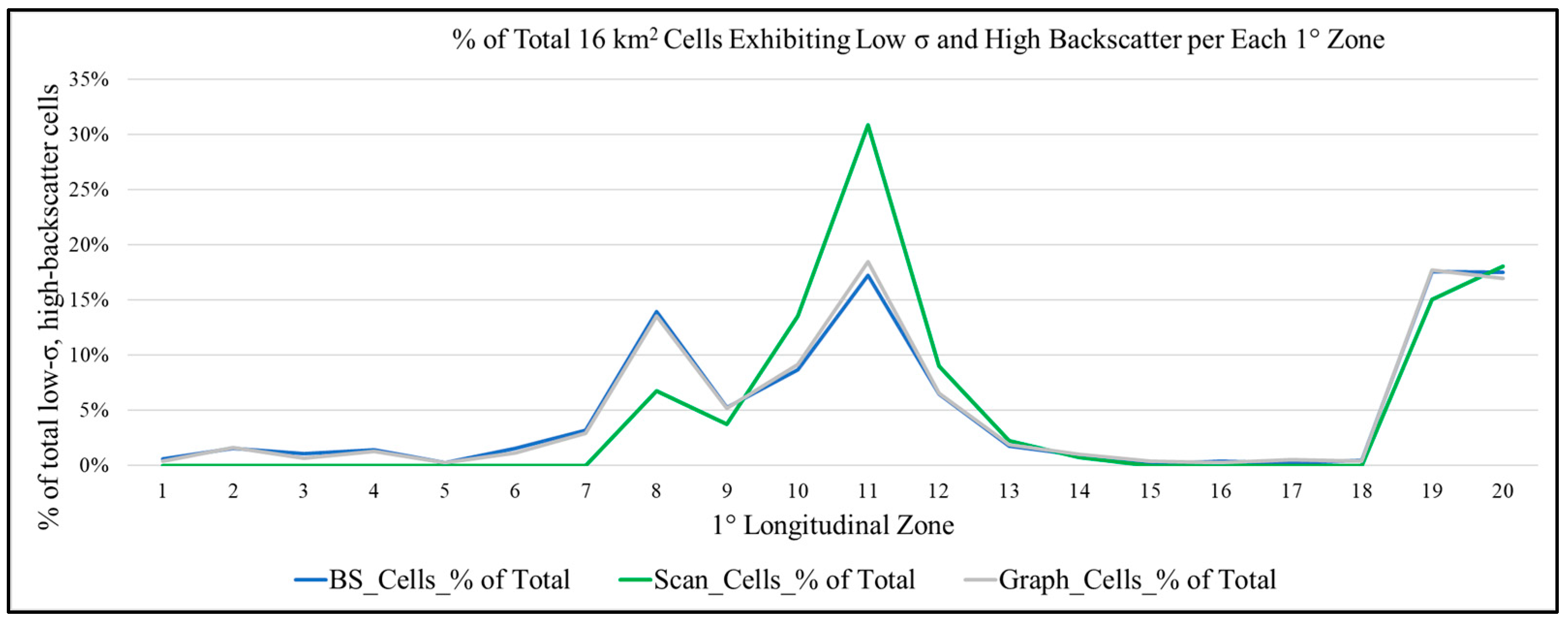
| 1° Longitude Zone | BS_Cells_% of Total | Scan_Cells_% of Total | Graph_Cells_% of Total |
|---|---|---|---|
| 1 | 0.59% | 0.00% | 0.38% |
| 2 | 1.52% | 0.00% | 1.63% |
| 3 | 1.06% | 0.00% | 0.63% |
| 4 | 1.41% | 0.00% | 1.25% |
| 5 | 0.23% | 0.00% | 0.25% |
| 6 | 1.52% | 0.00% | 1.13% |
| 7 | 3.17% | 0.00% | 2.89% |
| 8 | 13.95% | 6.77% | 13.55% |
| 9 | 5.28% | 3.76% | 5.14% |
| 10 | 8.68% | 13.53% | 9.16% |
| 11 | 17.23% | 30.83% | 18.44% |
| 12 | 6.45% | 9.02% | 6.52% |
| 13 | 1.76% | 2.26% | 1.88% |
| 14 | 0.94% | 0.75% | 1.00% |
| 15 | 0.12% | 0.00% | 0.38% |
| 16 | 0.35% | 0.00% | 0.25% |
| 17 | 0.23% | 0.00% | 0.50% |
| 18 | 0.47% | 0.00% | 0.38% |
| 19 | 17.58% | 15.04% | 17.69% |
| 20 | 17.47% | 18.05% | 16.94% |
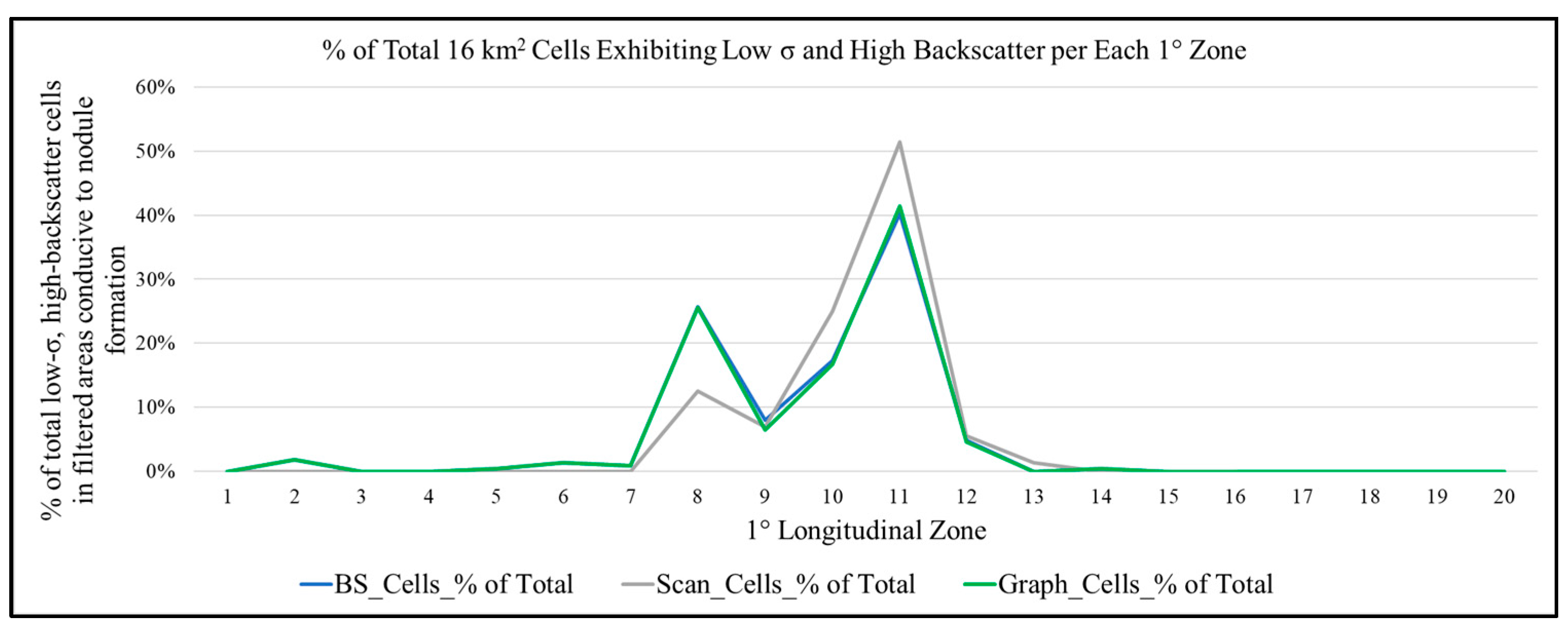
| 1° Longitude Zone | BS_Cells_% of Total | Scan_Cells_% of Total | Graph_Cells_% of Total |
|---|---|---|---|
| 1 | 0.00% | 0.00% | 0.00% |
| 2 | 1.77% | 0.00% | 1.86% |
| 3 | 0.00% | 0.00% | 0.00% |
| 4 | 0.00% | 0.00% | 0.00% |
| 5 | 0.44% | 0.00% | 0.47% |
| 6 | 1.33% | 0.00% | 1.40% |
| 7 | 0.88% | 0.00% | 0.93% |
| 8 | 25.66% | 12.50% | 25.58% |
| 9 | 7.96% | 6.94% | 6.51% |
| 10 | 17.26% | 25.00% | 16.74% |
| 11 | 40.27% | 51.39% | 41.40% |
| 12 | 4.87% | 5.56% | 4.65% |
| 13 | 0.00% | 1.39% | 0.00% |
| 14 | 0.44% | 0.00% | 0.47% |
| 15 | 0.00% | 0.00% | 0.00% |
| 16 | 0.00% | 0.00% | 0.00% |
| 17 | 0.00% | 0.00% | 0.00% |
| 18 | 0.00% | 0.00% | 0.00% |
| 19 | 0.00% | 0.00% | 0.00% |
| 20 | 0.00% | 0.00% | 0.00% |
| Site | Area Name | Mean BS (dB) | Absolute Difference Between Trendline Intercept and Nadir | Absolute Average Difference Between Trendline Intercept and BS at Incidence Angles |
|---|---|---|---|---|
| 1 | EPR | −19.69 | 8.687355 | 2.29 |
| 2 | Survey flat area between volcanic features west of EPR | −40.22 | 11.8692 | 1.75 |
| 3 | Transit southeast of/younger than Area A | −36.53 | 7.593326 | 2.91 |
| 4 | Transit slightly southeast of/younger than Area A | −23.49 | 10.575 | 2.73 |
| 5 | Area A | −19.283 | 1.283 | 1.10 |
| 6 | Transit slightly northwest of Area A | −28.5 | 4.996 | 4.65 |
| 7 | Kurchatov trough | −26.14 | 24.942 | 5.62 |
| 8 | Selkirk structure | −27.72 | 10.829983 | 3.29 |
| 9 | Transit north of Selkirk structure, apparent low BS | −39.42 | 4.057381 | 1.37 |
| 10 | Transit in northwest data area, apparent low BS | −42.05 | 9.019949 | 2.00 |
| Seafloor Strata Type | Mean BS (dB) | Absolute Difference Between Trendline Intercept and Nadir | Absolute Average Difference Between Trendline Intercept and BS at Incidence Angles |
|---|---|---|---|
| Pelagic Clay in Deep-Sea Basin | −37.16 | 15.40 | 7.25 |
| Calcareous Pelagic Sediment on Seamount Summit | −37.34 | 14.76 | 8.34 |
| Nodules ~20 kg/m2 | −30.51 | 12.12 | 6.29 |
| Nodules ~40 kg/m2 | −25.97 | 5.97 | 0.80 |
| Cobalt-rich Crusts on Seamount Flank and Summit | −24.85 | 3.03 | 1.83 |
| Debris Flow Sediment on Bottom of Seamount Flanks | −28.03 | 5.85 | 2.86 |
Disclaimer/Publisher’s Note: The statements, opinions and data contained in all publications are solely those of the individual author(s) and contributor(s) and not of MDPI and/or the editor(s). MDPI and/or the editor(s) disclaim responsibility for any injury to people or property resulting from any ideas, methods, instructions or products referred to in the content. |
© 2024 by the authors. Licensee MDPI, Basel, Switzerland. This article is an open access article distributed under the terms and conditions of the Creative Commons Attribution (CC BY) license (https://creativecommons.org/licenses/by/4.0/).
Share and Cite
Mussett, M.E.; Naar, D.F.; Caress, D.W.; Conrad, T.A.; Graham, A.G.C.; Kaufmann, M.; Maia, M. Analyzing Archive Transit Multibeam Data for Nodule Occurrences. J. Mar. Sci. Eng. 2024, 12, 2322. https://doi.org/10.3390/jmse12122322
Mussett ME, Naar DF, Caress DW, Conrad TA, Graham AGC, Kaufmann M, Maia M. Analyzing Archive Transit Multibeam Data for Nodule Occurrences. Journal of Marine Science and Engineering. 2024; 12(12):2322. https://doi.org/10.3390/jmse12122322
Chicago/Turabian StyleMussett, Mark E., David F. Naar, David W. Caress, Tracey A. Conrad, Alastair G. C. Graham, Max Kaufmann, and Marcia Maia. 2024. "Analyzing Archive Transit Multibeam Data for Nodule Occurrences" Journal of Marine Science and Engineering 12, no. 12: 2322. https://doi.org/10.3390/jmse12122322
APA StyleMussett, M. E., Naar, D. F., Caress, D. W., Conrad, T. A., Graham, A. G. C., Kaufmann, M., & Maia, M. (2024). Analyzing Archive Transit Multibeam Data for Nodule Occurrences. Journal of Marine Science and Engineering, 12(12), 2322. https://doi.org/10.3390/jmse12122322