Research on the Lossless Data Compression System of the Argo Buoy Based on BiLSTM-MHSA-MLP

Abstract

This study addresses the issues of the limited data storage capacity of Argo buoys and satellite communication charges on the basis of data volume by proposing a block lossless data compression method that combines bidirectional long short-term memory networks and multi-head self-attention with a multilayer perceptron (BiLSTM-MHSA-MLP). We constructed an Argo buoy data compression system using the main buoy control board, Jetson nano development board, and the BeiDou-3 satellite transparent transmission module. By processing input sequences bidirectionally, BiLSTM enhances the understanding of the temporal relationships within profile data, whereas the MHSA processes the outputs of the BiLSTM layer in parallel to obtain richer representations. Building on this preliminary probability prediction model, a multilayer perceptron (MLP) and a block length parameter (block_len) are introduced to achieve block compression during training, dynamically updating the model and optimizing symbol probability distributions for more accurate predictions. Experiments conducted on multiple 4000 m single-batch profile datasets from both the PC and Jetson nano platforms demonstrate that this method achieves a lower compression ratio, shorter compression time, and greater specificity. This approach significantly reduces the communication time between Argo buoys and satellites, laying a foundation for the future integration of Jetson Nano into Argo buoys for real-time data compression.

1. Introduction

The ocean covers 70% of the Earth’s surface and is the richest resource reservoir. The sustainable development and security of the ocean are crucial to global interests, and ocean exploration technology plays an important role in this. The collection of various ocean data through ocean exploration instruments can help humans fully understand the ocean [1,2]. Commonly used detection instruments include underwater gliders, Argo buoys, and underwater robots. Among them, Argo buoys are the most widely used for collecting ocean profile data [3]. The Chinese Argo Program is one of the key foundations for China’s marine science research and development, and it is also an important part of the international ocean observation network [4]. Argo buoys collect data based on marine environmental factors to accurately understand the laws of the ocean, improve the accuracy of climate forecasts, and effectively reduce the threats posed to humans by various marine and climate disasters [5]. Argo buoys are equipped with a variety of sensors to collect a variety of ocean information during the profiling process, playing an irreplaceable role in ocean monitoring. As their functions become increasingly complete and their endurance increases, the amount of data they collect also increases greatly, which places higher requirements for the data storage and transmission of the buoy system.

Ocean buoys generally use satellite communications to transmit data and report their positions to ground-based platforms. With the successful launch of the last BeiDou-3 satellite in June 2020, the BeiDou-3 satellite was completed. Its communication range can cover the entire world and greatly improve the communication capabilities of China and its surrounding areas [6]. Therefore, BeiDou-3 satellites play an important role in the data transmission and communication of Argo buoys. The Argo buoys upload the collected single batch of profile data to the satellite via the BeiDou-3 transparent transmission module at 228 bytes at an interval of 65 s, and then the satellite transmits the collected data to the ground-based platform. However, the buoy data storage capacity is limited, and satellite communications are generally charged by volume. Therefore, it is necessary to compress the profile data via a lossless data compression algorithm based on the characteristics of the data before they are uploaded to the satellite, which is very important for improving transmission efficiency and reducing satellite communication costs.

Due to the high accuracy requirements of deep-sea profile data, this study focuses exclusively on lossless compression methods, which ensure that the data remains completely identical before and after compression and decompression. Current compression algorithms are mainly divided into dictionary coding and entropy coding [7]. At present, the mainstream dictionary coding algorithm is the Lempel-Ziv (LZ) [8,9] series algorithm. Although these algorithms can remove redundancy in data, their compression efficiency is low, and the implementation of encoding and decoding is relatively complex, especially due to the need to maintain a dynamic dictionary. Cheng [10] applied the improved Lempel-Ziv-Welch (LZW) compression algorithm to the sonar buoy signal acquisition system, achieving a compression ratio between 54% and 60%. Compared to the conventional LZW compression algorithm, it demonstrated a significant reduction in compression ratio. Cleary et al. [11] proposed the prediction by partial matching (PPM) compression algorithm, which is a lossless compression algorithm based on context modeling. Its core idea is to use known contextual information to predict the probability distribution of the next symbol. However, it requires complex probability estimation and context modeling, so it requires high computing speed and high memory consumption. In addition, it has poor adaptability when processing data without obvious statistical regularities. Barina [12] inserted phrases into the dictionary of the x3 compressor to reduce the compression ratio. Notably, x3 is a lossless optimized dictionary-based data compressor.

Entropy coding methods include Huffman coding [13,14,15] and arithmetic coding [16,17]. The Bzip2 [18] compression algorithm combines block sorting compression and Huffman coding techniques, where block sorting compression improves the matching efficiency of the duplicate data by sorting the input data, and Huffman coding is used for entropy coding of these matched data. The move-to-front predictive coding (Mtfpc) algorithm encodes symbols via a probability model and contextual information to achieve higher compression efficiency, making it a compression algorithm that is based on entropy coding. Hu et al. [19] applied Huffman coding and the LZW algorithm to buoy communication compression, with compression ratios of 45% and 55%, respectively. The compression ratio is relatively high, and there is much room for improvement. Nasif et al. [20] proposed a new lossless Huffman deep compression (HDC) algorithm, which combines sliding window technology to adapt to memory, uses deep learning pruning and pooling technology to reduce the complexity of the Huffman tree, and utilizes pattern matching and weights to achieve greater compression. Huffman coding cannot reach the entropy limit, whereas arithmetic coding can represent a set of characters as floating-point numbers in the interval [0, 1] through a probability distribution, which is closest to the entropy limit [21]. Therefore, this paper uses arithmetic coding for lossless data compression.

With the development of deep learning, probabilistic prediction algorithms have been rapidly applied. The essence of lossless data compression is also a probabilistic statistical model, so deep learning has achieved good application in data compression. Yamagiwa et al. [22] applied principal component analysis (PCA) and a deep neural network (DNN) for image compression and achieved a good compression ratio. Tatwawadi [23] introduced the recurrent neural network (RNN) into a lossless data compression model and achieved good results. However, the traditional RNN has problems such as gradient vanishing and explosion, long-distance dependency, and difficulty in parallelization. Qu et al. [24] proposed a lossless compression method based on the gated recurrent unit (GRU). Although it alleviates the vanishing and exploding gradient problems, it still faces the problems of long-distance dependency and inability to parallelize. Goyal et al. [25,26] proposed a variety of lossless compression models based on long short-term memory (LSTM) variants and achieved good compression results. Among them, bidirectional long short-term memory (BiLSTM) can capture the dependency between the context in the input sequence, thereby improving the model’s ability to understand the sequence. Although it alleviates the long-term dependency problem, it is still difficult to parallelize. The emergence of the attention mechanism [27] thus solved the abovementioned problem of parallelization difficulty. Bellard [28] used Transformer as a probabilistic prediction model and achieved good results on multiple large datasets. Although Transformer has strong representation and parallel computing capabilities, it is large and complex, has a long training cycle, has excessive performance, and has average results on smaller single-batch profile datasets. E et al. [29] used Transformer and a bidirectional gated recurrent unit as probability predictors, and they compared them with two traditional lossless compression methods, arithmetic coding and dictionary-based LZW, to reduce the compression ratio. In addition to dictionary and entropy coding, floating-point encoding has also been widely applied in data compression. Wang et al. [30] proposed an efficient lossless compression algorithm for time-series floating-point data based on existing compression methods, and they significantly improved the compression efficiency of time-series floating-point numbers through three optimization strategies. After optimization, the compression ratio was increased by an average of 12.25%, achieving a significant performance improvement.

This paper proposes a block lossless data compression method based on bidirectional long short-term memory networks and multi-head self-attention combined with a multilayer perceptron (BiLSTM-MHSA-MLP). The preliminary probability prediction model (BiLSTM-MHSA) integrates bidirectional LSTM and multi-head self-attention layers. BiLSTM, as an extension of LSTM, enhances the understanding and capture of temporal relationships within sequences by processing input sequences bidirectionally. The MHSA processes the outputs of BiLSTM in parallel, focusing on different parts to obtain richer representations, reduce information loss, and capture more details and semantic information. Additionally, a multilayer perceptron (MLP) and a block length parameter (block_len) are introduced on top of the trained preliminary probability prediction model, enabling block compression during training. This approach dynamically updates the model and optimizes the symbol probability distributions, providing more accurate predictions. Finally, the compression algorithm is successfully ported to the Jetson nano development board, achieving lossless data compression on both the PC and the Jetson nano platforms.

2. Probabilistic Prediction Models

2.1. Bidirectional Long Short-Term Memory Network Model

A long short-term memory (LSTM) network controls the flow of information by introducing memory units and gating mechanisms, thereby solving the gradient vanishing and exploding problems in traditional RNNs and improving the ability to capture the long-term dependencies of sequences. The forget gate determines how much of the memory cell state of the previous time step needs to be retained and how much needs to be forgotten. The input gate determines how much of the input information of the current time step needs to be added to the memory cell state. The update of the memory cell state is based on the output of the forget gate and the input gate to update the memory cell state of the current time step. The output gate determines which part of the current memory cell state will be output, and it combines the hidden state to form the output of the current time step. The unidirectional LSTM processes input sequentially in time order and in a forward direction, and the output of each time step depends only on the current time step and the previous time step. It may not be able to fully capture the sequence symmetry and utilize contextual information, so BiLSTM is introduced. BiLSTM is an extension of LSTM. By processing the input sequence in both directions, it can better understand and capture the symmetrical information and dependencies in the sequence. This paper uses a single-layer bidirectional long short-term memory network unit to perform sequence modeling and feature extraction on the output of the embedding layer. BiLSTM consists of two LSTM layers, one processing the forward sequence and the other processing the backward sequence. The BiLSTM network architecture is shown in Figure 1.

Where X is the output of the input data after the embedding layer, and its dimensions are (batch_size, timesteps, emb_size). Y is the output of the BiLSTM layer, with dimensions of (batch_size, timesteps, lstm_size × 2). Y contains rich contextual information about the input data.

2.2. Multi-Head Self-Attention Network Model

The output Y of the BiLSTM layer is input into the multi-head self-attention (MHSA) layer, which enhances the performance of the model by computing multiple attention heads in parallel. Each attention head learns different information through different linear transformations, thereby capturing a variety of different contextual relationships and dependencies in the sequence. In this paper, there are h attention heads. First, the sequence $Y$ is linearly transformed using different weight matrices to generate query ($Q_i$), key ($K_i$), and value ($V_i$) vectors. Each attention head has an independent weight matrix. The formulas for calculating the query, key, and value vectors are as follows:

$$Q_i=Y{W}_{Q_i}$$

(1)

$$K_i=Y{W}_{K_i}$$

(2)

$$V_i=Y{W}_{V_i}$$

(3)

The value of $i$ ranges from 1 to h, and $W_{Q_i}$, $W_{K_i}$, and $W_{V_i}$ are weight matrices.

The self-attention mechanism is then executed on each attentional head to obtain the output of each $hea{d}_i$, calculated as follows:

$$hea{d}_i=Attention(Q_i,K_i,V_i)=Soft\max ({\displaystyle \frac{Q_i{K}_i^T}{\sqrt{d_k}}})V_i$$

(4)

where $d_k$ is the dimension of the key vector used to scale the scores.

Finally, the outputs of all the attention heads are concatenated to obtain the output $M$, as shown in Equation (5).

$$M=MultiHead(Q_i,K_i,V_i)=Concat(hea{d}_1,\dots ,hea{d}_h)W_O$$

(5)

where $W_O$ is the output linear transformation matrix.

Through the above formulas and steps, the MHSA can process the output sequence Y of the BiLSTM layer in parallel. Each attention head of the MHSA layer learns features in different subspaces, which enables the model to understand the relationships in the input sequence from different perspectives. By merging the attention information from different heads, the model can comprehensively consider different types of contextual information and more comprehensively understand the dependencies in the sequence. Compared with single-head attention, the multi-head attention mechanism obtains richer representations by focusing on different parts multiple times, thus reducing information loss and helping capture more details and semantic information. This mechanism plays a vital role in the probability prediction model presented in this paper. The output of the MHSA layer is $M$, whose dimensions are (batch_size, timesteps, lstm_size × 2).

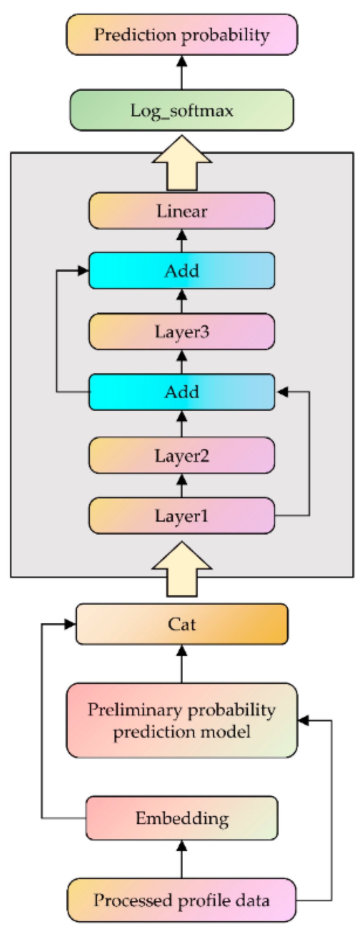
2.3. Preliminary Probability Prediction Model

The structure of the preliminary probability prediction model is shown in Figure 2. The output of the MHSA layer is $M$. The Linear1 linear layer is introduced to reduce the dimension of the output of the MHSA layer and output it as $M_1$. The calculation formula of $M_1$ is shown in Equation (6). The GELU nonlinear transformation is introduced, and its output is $M_2$. The calculation formula of $M_2$ is shown in Equation (7). The GELU function is selected as the activation function of the preliminary probability predictor. The GELU function is smooth over the entire real number domain, which helps reduce the gradient vanishing problem, especially in deep neural networks. The Linear2 linear layer maps the learned features to the vocabulary space, generating a tensor in which each element represents the score of a token in the vocabulary. The output of this layer is $M_3$. The calculation formula of $M_3$ is expressed by Equation (8).

$$M_1=W_{1}M+b_1$$

(6)

$$M_2=GELU(M_1)$$

(7)

$$M_3=W_2{M}_2+b_2$$

(8)

where $W_1$ and $W_2$ and $b_1$ and $b_2$ are the weight parameters and bias, respectively, and the dimension of $M_3$ is (batch_size, vocab_size).

To facilitate the calculation of losses, the Log_Softmax function is used to convert the original output of the model into logarithmic probability. The Log_Softmax function can avoid the numerical instability problem caused by the exponential function during the calculation process, especially when the logit value is very large or very small.

The introduction of the BiLSTM layer can provide richer contextual information and improve the model’s ability to model sequence data. The combination of the forward and backward information of the BiLSTM makes the representation input to the MHSA layer more complete, which helps generate more accurate attention weights, thereby improving the model’s focus on key parts. The MHSA layer can consider the information of all other time steps in the sequence when calculating the output of each time step. In this way, the model can dynamically adjust the representation of each time step to include more contextual information. In addition, the MHSA layer allows for multiple attention heads to be calculated in parallel, which can improve the computational efficiency of the preliminary probability model. Therefore, through the combination of the BiLSTM layer and the MHSA layer, not only are the position information and modeling capabilities enriched, but also the understanding of the context is enhanced, and the performance of the model in compression tasks is improved.

2.4. Probabilistic Prediction Model

Although the preliminary probability prediction model has achieved a reduction in the compression ratio compared with traditional compression algorithms and traditional deep learning compression algorithms, there has been no significant improvement in the compression time. Therefore, on the basis of the construction and training of the preliminary probability prediction model, an MLP and block_len are introduced to realize the training and block compression of deep-sea profile data. The MLP extracts and transforms features through multiple fully connected layers and nonlinear activation functions to generate the final prediction. This structure can dynamically update the model during the compression process, gradually adapt to the data distribution, and provide more accurate probability predictions, thereby reducing the compression ratio and shortening the compression time. The complete probability prediction model structure is shown in Figure 3.

First, the single batch of profile data to be compressed is added to the embedding layer, which converts the input data into the corresponding embedding vectors, which can effectively capture the semantic relationship between the data and convert discrete text data into continuous vectors that can be input into the neural network. Moreover, the single batch of profile data to be compressed is input into the trained preliminary probability prediction model to obtain the output result of the Linear1 linear layer in the model and transform its dimension to (batch_size, −1). The output result of the word embedding layer is concatenated with the result of the preliminary probability prediction model to form a new tensor, which contains rich information from the preliminary probability prediction model, thereby enhancing the feature fusion capability.

Second, the tensor is input into the MLP network model, which includes three layers, two layers of residual networks and one layer of a linear transformation layer. All three layers use LeakyReLU as the activation function and the slope parameter is 0.005. Because the leaky ReLU function has a small gradient in the negative part, it can solve the problem of neuron death in the ReLU function. Moreover, it is sensitive to the slope parameter and needs to be adjusted. Layer1 consists of one linear layer and one activation function layer; Layers 2 and 3 are both composed of two linear layers and two activation functions. The introduction of multiple fully connected layers can significantly increase the expressiveness of the model. By stacking multiple nonlinear activation functions, the multilayer fully connected network enables the model to better capture complex patterns and nonlinear relationships in the data. The introduction of nonlinearity enables the network to learn more complex function mappings, thereby improving the expressiveness of the model. The introduction of residual networks helps alleviate the vanishing gradient problem. Residual connections allow gradients to flow more easily during back propagation. In addition, the use of residual connections can accelerate the training process of the model. The design of the residual network allows the function learned by each layer to be regarded as a “correction” of the input, which allows each layer to learn only the changes in the input instead of the complete representation, thereby simplifying the learning task and promoting faster convergence. Therefore, the combination of multilayer fully connected networks and residual connection networks can improve the stability of the model. Through the above changes, the dimension of the output of the second layer residual network is (batch_size × block_len, hdim).

Finally, the linear layer is used to map the learned features to the letter space, generating a tensor in which each element represents the score of a token in the alphabet. The output dimension is (batch_size × block_len, vocab_size). As with the preliminary probability prediction model, the Log_Softmax function is used to convert the original output of the model into log probability, which is combined with negative log-likelihood loss to achieve model optimization. The specific model parameters are shown in

Table 1. Probabilistic model parameters.

Parameter Name	Parameter Size
batch_size	64
timesteps	64
emb_size	32
lstm_size	128
h	8
vocab_size	14
block_len	12
hdim	1024

.

3. Data Compression and Decompression

3.1. Adaptive Arithmetic Coding

Arithmetic coding, like Huffman coding, is a probability-based lossless data compression technology. Huffman coding requires counting the frequencies of all the symbols in advance and building a Huffman tree on the basis of these frequencies. This means that the entire message must be scanned before encoding, which may be impractical for large files or real-time data streams. In addition, Huffman coding also has disadvantages such as limited compression efficiency and complex decoding. Arithmetic coding can approach the entropy limit of data, that is, the theoretical minimum compression size; at the same time, it is applicable to various symbol probability distributions, especially when the symbol probability is uneven. Therefore, arithmetic coding has the advantages of a high compression rate and strong adaptability. This article uses arithmetic coding to achieve profile data compression. Arithmetic coding achieves compression by representing the entire message as a real number interval. The range of this interval is between 0 and 1, and each symbol in the message is represented by gradually reducing the interval.

On the basis of the different symbol probability estimation methods, arithmetic coding can be divided into static arithmetic coding and adaptive arithmetic coding [31]. Static arithmetic coding must perform statistics on the entire message before encoding to determine the probability distribution of each symbol. This requires additional time and computing resources, and this preprocessing step may be impractical, especially for large files or real-time data streams. In addition, static arithmetic coding is not applicable to large-scale data or real-time data streams. Therefore, this paper adopts adaptive arithmetic coding to realize source coding. Adaptive arithmetic coding (AAC) is a lossless compression algorithm that dynamically adjusts the probability distributions of symbols. During the encoding process, it does not require the precalculation of the probability distribution of symbols, but dynamically updates the probability distribution on the basis of the actual occurrence of the data stream [24].

3.2. Profile Data Preprocessing

First, to facilitate subsequent reading and training, the collected profile data in the txt format is converted into an npy file. The raw profile data is read character by character, and each unique character is assigned a unique identifier. Different characters are given different identifiers, and the total number of identifiers determines the size of the alphabet. Two dictionaries are also generated, one mapping characters to identifiers and another mapping identifiers to characters. These dictionaries will be used for character matching in later stages. Using the constructed dictionaries, the raw profile data are then converted into an integer-based npy file, one character at a time.

Second, the npy file is divided into a 2D training array using a sliding window and the introduction of timesteps. The file is split into features X and labels Y. In this paper, the probability of the timesteps+1st character is estimated by the previous timestep characters. Assuming the character sequence of the training data npy file is $S^N=\{S_1,S_2,\dots ,S_N\}$, and that the file has N characters, the character stream is first read from the npy file and reshaped into a 1D character vector. Then, using a sliding window and time steps, the 1D vector is split into an overlapping segmented matrix of shape (n, timesteps + 1), as shown in Figure 4.

The first timestep columns of the overlapping segmentation matrix are used as feature X, and the last column is used as label Y. The number of rows n of the overlapping segmentation matrix is the number of training samples, and the dimensions of feature X of each training sample are the timesteps.

Finally, the obtained X and Y are used to generate a dataset through DataLoader. Data can be obtained batch by batch later to speed up model training.

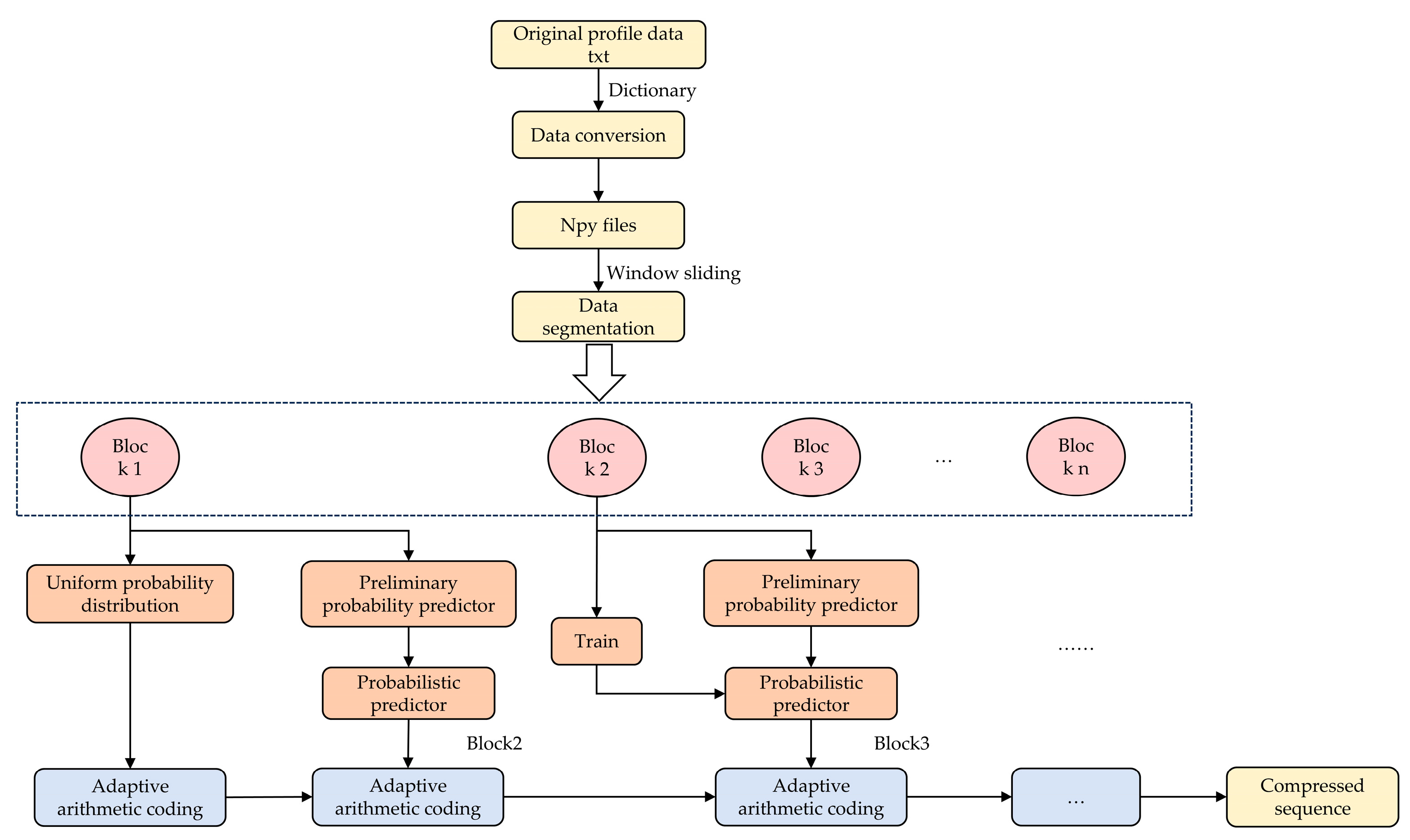
3.3. Compression and Decompression Model

This paper uses an adaptive arithmetic coding module to achieve compression and decompression. For the initial timesteps, a uniform probability distribution is adopted, and adaptive arithmetic coding is performed to achieve lossless compression. The timestep characters are subsequently passed through the preliminary probability prediction module and the probability prediction module to predict the probability distributions of other characters. The adaptive arithmetic coding module updates the cumulative frequency table and the original character probability distribution according to the probability distribution and the timesteps+1st character to obtain new probability intervals for other characters. By looping this process, the probability interval of the Nth character can be obtained, and the encoding is then completed. Among them, block 1 refers to the initial timesteps of the column data of each batch, block 2 to block n − 1 refer to block_len × batch_size data, block_len defines the number of time steps processed in each iteration, batch_size indicates the number of samples in each batch, and block n refers to the remaining data in the end. The compression flow chart is shown in Figure 5. The overall compression process is shown in pseudocode as Algorithm 1.

Algorithm 1: Compression algorithm

1: Input:

2: input_data: data to be compressed

3: timesteps: number of timesteps in each sequence

4: model: probability prediction model

5: Output:

6: com_data: compressed data

7: params: model parameters

8: Initialize parameters:

9: params.append (char2id_dict, id2char_dict)

10: integer_encoded ← Encode (input_data, char2id_dict)

11: params.append (len(integer_encoded))

12: [train_x, train_y] ← ExtractFeaturesAndLabels(integer_encoded, timesteps)

13: Encode the initial timesteps with a uniform distribution:

14: for i ← 0 to timesteps do

15:  com_data.append (ArithmeticEncoder (train_y [0, i], uniform))

16: end for

17: Process remaining data:

18: for j ← 0 to len(train_x) do

19:  prob ← model.predict (train_x[j])

20:  com_data.append (ArithmeticEncoder(train_y[j], prob))

21: end for

22: End:

23: Return com_data and params

During the data compression process, the preliminary probability predictor is composed of a BiLSTM network and an MHSA network, which is trained and saved via the 4000 m profile dataset collected by the deep-sea Argo buoy. The probability predictor is based on the preliminary probability predictor and adds an MLP network, which includes multiple fully connected layers and residual network layers. Block_len is introduced during compression to achieve block compression and training, which determines the frequency of model updates and the length of the encoding symbol block. This approach strikes a balance between the model update frequency and computational efficiency. A smaller block length means more frequent model updates, which may lead to better compression effects, but the computational cost is relatively high. When the data volume reaches block_len × batch_size, the data are sent to the probability predictor and adaptive arithmetic coding module to complete data compression. At the same time, the data are also used to train the probability prediction model. During the compression process, the parameter requires_grad of the preliminary probability prediction model is set to False to prevent the trained preliminary probability prediction model from being updated. The introduced MLP network is trained during the compression process so that the probability prediction model is dynamically updated and gradually adapts to the distribution of compressed data, thereby providing more accurate predictions.

The decompression process is symmetrical to the compression process. First, the initial timesteps are arithmetically decoded via a uniform probability distribution. Then, the probability of the timesteps+1st character is output by the prestored probability predictor on the basis of the first timestep characters. The probability distribution and cumulative frequency table are updated using this probability and the character, and the character is decoded according to the probability interval into which it falls. This process can be repeated to decompress N characters. The decompression process is shown in Figure 6. Finally, the decompressed characters are restored to the original deep-sea profile txt file through the previously constructed dictionary. The overall decompression process is shown in pseudocode as Algorithm 2.

Algorithm 2: Decompression algorithm

1: Input:

2: com_data: compressed data

3: timesteps: number of timesteps in each sequence

4: model: probability prediction model

5: params: model parameters

6: Output:

7: decom_data: decompressed data

8: Initialize parameters:

9: char2id_dict, id2char_dict, len_series ← params[0], params[1], params[2]

10: Decode the initial timesteps with a uniform distribution:

11: for i ← 0 to timesteps do

12:  data ← ArithmeticDecoder (com_data, uniform)

13: end for

14: Process remaining data:

15: for j ← timesteps to len_series do

16:  train_x ← data (j—timesteps, j)

17:  prob ← model.predict (train_x)

18:  data.append (ArithmeticDecoder(com_data, prob))

19: end for

20: Transform decoded data:

21: decom_data ← transform (data)

22: End:

23: Return decom_data

3.4. Argo Buoy Data Compression System Design

The Jetson nano development board is a low-cost AI computer launched by NVIDIA, which has high performance and energy efficiency, as shown in Figure 7.

In data compression algorithms, a lower compression ratio results in more compact data, but it usually means a more complex computational process is required, which increases computational overhead. However, considering that the single batch profile data from Argo buoys is typically smaller than 5000 bytes, the data volume is relatively small, and the Jetson nano can efficiently handle such data without facing significant computational resource bottlenecks. The Jetson nano is equipped with a quad-core ARM Cortex-A57 CPU and a 128-core NVIDIA Maxwell GPU, with excellent performance in processing small-scale data, particularly in deep learning inference tasks, ensuring efficient computation. Although BiLSTM and MHSA modules are computationally intensive, for a small dataset of only 5000 bytes, the Jetson nano’s GPU effectively reduces computation time, keeping the computational overhead within an acceptable range and avoiding issues like memory shortages or overload. In the compression task, the BiLSTM and MHSA models have been pre-trained on the Argo buoy’s training data, and the model weights and structure are stored on the SD card. During inference, Jetson Nano loads the pre-trained model into the main memory for computation. Since the data size for each batch is small, Jetson Nano can efficiently load and execute the inference tasks, ensuring that the computational resource requirements for the data compression process are low, with short runtime, thus resulting in the limited consumption of battery and computational resources. As a low-power edge computing platform, Jetson nano can execute computationally intensive tasks while saving energy. In the application of Argo buoys in ocean exploration, Jetson nano, with efficient compression technology, reduces bandwidth demands, lowers transmission costs, and enhances data transmission efficiency. This is particularly advantageous for floats with limited battery and bandwidth resources, significantly improving the efficiency of data collection and transmission. Therefore, the Jetson nano development board is selected as the hardware environment for buoy lossless data compression. It configures the software environment for deep learning and lossless data compression by loading the Ubuntu 18.04LTS system.

The Jetson nano development board communicates with the Argo buoy’s main control board via UART using the 40 Pin IO pin ttyTHS1. First, the Jetson nano board powers on and automatically runs the main_com.py file. It executes the power_on function, sending the $JPWR,1,* command via the ttyTHS1 serial port to the main control board to confirm power-on completion. Then, it runs the rec_data function to wait for commands from the main control board. The main control board transmits profile data stored on the SD card to the Jetson nano via the UART4 serial port in $MESS,N,1,256 bytes,* format (where N is the total number of packets, and 1 is the current packet number) at intervals of 50 milliseconds per packet. The Jetson nano receives the data, verifies the $MESS message header, extracts the 256-byte data, and saves them as a txt file. If the $MESS message header is not received or the message format is incorrect, the Jetson nano will discard the message. Once data transmission is complete, the main control board sends the $COMP,1,* command to notify the Jetson nano that data transmission has ended. Upon receiving the command, the Jetson nano initiates data compression by executing the command python3 /home/zhang/compytorch/start_com.py. Before starting compression, it sends the $COMP,1,* command via the ttyTHS1 serial port to inform the main control board that data compression is about to begin. Then, the Jetson nano executes the command source ~/.virtualenvs/pytorch/bin/activate && cd /home/zhang/compytorch && python3 cb_txt.py && deactivate to perform data compression, where source ~/.virtualenvs/pytorch/bin/activate means entering the pytorch virtual environment, cd /home/zhang/compytorch means navigating to the specified folder compytorch, python3 cb_txt.py means executing the compression program cb_txt.py, and deactivate means exiting the virtual environment. After compression is completed, it sends the $FINC,1,* command via the ttyTHS1 serial port to notify the main control board that compression is complete. Upon receiving the command, the main control board responds with the $SFND,1,* command, allowing the Jetson nano to send the compressed data. Subsequently, the Jetson nano transmits the compressed data back to the main control board via the ttyTHS1 serial port in the $MESS,M,1,220 bytes,* format (where M is the total number of packets, and 1 is the current packet number) at a rate of 220 bytes per second. The Jetson nano development board sends the command $FINS,1,* to notify the main control board that the transmission of the compressed data is complete. The main control board saves the received compressed data and forwards them to the BeiDou-3 transparent transmission module via the USART2 serial port. The BeiDou-3 module sends the compressed data to the satellite in chunks of 228 bytes with an interval of 65 s. Finally, the satellite relays the received data to the ground-based platform, where the data are decompressed on a PC. The specific module communication process is shown in Figure 8. The hardware connection of the Argo buoy compression system is shown in Figure 9.

4. Results and Discussion

4.1. Data Preparation

The preliminary probability prediction model of this study was trained on a dataset of approximately 4000 4000 m single-batch profiles collected by the laboratory’s deep-sea Argo buoy. The PC environment is Python 3.9 with torch 1.10.0 and torchvision 0.11.0. The Jetson nano environment is Python 3.8 with torch 1.8.0 and torchvision 0.9.0. Twelve 4000 m single batch profile datasets were used for experimental verification on the PC and Jetson nano development board. The experimental data are shown in

Table 2. The 4000 m single batch profile data.

Number	4000 m Profile Data	Data Size (Bytes)
D1	4000 m data 1	4486
D2	4000 m data 2	4486
D3	4000 m data 3	4520
D4	4000 m data 4	4486
D5	4000 m data 5	4520
D6	4000 m data 6	4486
D7	4000 m data 7	4554
D8	4000 m data 8	4520
D9	4000 m data 9	4520
D10	4000 m data 10	4588
D11	4000 m data 11	4588
D12	4000 m data 12	4486

. The composition of the 4000 m profile data are shown in

Table 3. The 4000 m profile data table.

4000 m Profile Data (Time, T/°C, D/m, C/μS/cm)
211217173303, 01.3692, 4002.8, 0418
211217174814, 01.3698, 3897.8, 0433
..........................................................
..........................................................
211218033031, 28.0043, 0002.6, 0866
211218033053, 28.0401, 0001.6, 0866

.

4.2. Experimental Verification of the Block_Len Parameter

On the basis of the preliminary probability prediction model, an MLP module and a block_len module are introduced to achieve block compression while training. The block_len parameter is used to determine the frequency of model updates and controls the amount of data processed at each step. Its size directly affects the model’s performance, context capturing ability, and training efficiency, balancing the frequency of model updates with computational efficiency. A smaller block_len can only capture short-term local context, which may overlook long-term dependencies. This limits the model’s ability to capture long-term relationships, but more frequent updates may lead to increased I/O and computational overhead, reducing training efficiency. Additionally, a smaller context window may reduce the model’s encoding ability. A larger block_len can capture a broader time range of context, helping the model better learn long-term dependencies. However, if block_len is too large, it may increase model complexity, significantly raise computational resource demands, and potentially lead to issues like insufficient memory or unstable gradients. In summary, the choice of block_len requires a trade-off between context capturing ability and computational resource demands. A smaller block_len provides more frequent model updates but may sacrifice long-term dependency capture, while a larger block_len allows for better long-term dependency capture, enhancing context understanding, but it may increase computational load and impact training efficiency.

In the context of data compression, the block_len parameter is introduced to implement block-wise compression, where each block contains block_len × batch_size data. Dividing data into smaller chunks can make computations more efficient and avoid over-loading memory. Chunking compression can also reduce the risk of numerical instability during computations. In addition, after compressing these data, they are also used for model training to gradually update the MLP model. This progressive training method allows the model to gradually adapt when processing new data, improves the learning effect of the model, and thus achieves a more efficient compression of new data. In this experiment, the values of block_len are 11, 12, 13, 14, and 15, and they are compared with those of the preliminary probability prediction model (BiLSTM-MHSA) in terms of the compression ratio and compression time. The specific comparison results are shown in Figure 10 and Figure 11.

As shown in Figure 10 and Figure 11, introducing the MLP on the basis of the BiLSTM-MHSA to achieve block compression while training can reduce the compression ratio and shorten the compression time. The minimum compression ratio of BiLSTM-MHSA is 12.98%, the average compression ratio is 13.37%, and the average compression time is 6.9 s. The experiment shows that when block_len is 12, the compression ratio is the lowest, the compression time is relatively short, and the compression effect is the best at this time. The lowest compression ratio is 12.03%, the average compression ratio is 12.11%, and the average compression time is 4.4 s. By comparison, the compression algorithm (BiLSTM-MHSA-MLP) adopted in this paper has an average compression ratio reduced by 1.26% and an average compression time reduced by 2.5 s compared with directly using BiLSTM-MHSA, indicating that the improved probability prediction model has stronger performance.

4.3. Comparison of the Compression Effects on PC and Jetson Nano

To realize the real-time lossless data compression of the Argo buoy in the future, it is necessary to transplant the compression algorithm in this paper to the Jetson nano development board. To verify the performance of the compression algorithm on the Jetson nano development board, the 12 groups of data in Table 2 are compressed on the PC and Jetson nano, respectively, and the compression ratio and compression time are compared. The specific comparison results are shown in Figure 12 and Figure 13.

As shown in the above figures, the average compression ratios of the PC and Jetson nano are both approximately 12.11%, which are basically the same. Owing to the difference in hardware architecture between Jetson nano and PC, there is a slight difference in the size of the compressed file. The average compression time on the PC is 4.4 s, and the average compression time on Jetson nano is 36.6 s. Compared with the PC, the average compression time is increased by 8.3 times, which is within an acceptable range. The compressed file of the above Jetson nano is sent to the PC through the serial port, and decompression is completed on the PC. The file is consistent with the one before compression, indicating that the compression algorithm presented in this paper enables lossless data compression.

4.4. Comparison of the Compression Effects of the BiLSTM-MHSA-MLP Algorithms

To verify the effectiveness of the compression algorithm in this paper, traditional compression algorithms (Huffman, LZW, PPM [11], Bzip2 [18] and Mtfpc), traditional deep learning compression algorithms (BiGRU [23], GRU_Multi [24], BiLSTM [25], LSTM_Multi [24], Transformer [27] and MHSA-MLP), and popular compressors (ZIP, 7Z, TGZ and GZ) are used to compress the five 4000 m single-batch profile datasets D1, D3, D5, D7, and D9, as shown in Table 2, and the compression ratio and compression time are calculated. First, the compression ratio is compared with those of traditional compression algorithms (Huffman, LZW, PPM, Bzip2 and Mtfpc). The test results are shown in Figure 14.

As shown in Figure 14, the preliminary probability prediction model (BiLSTM-MHSA) and the probability prediction model (BiLSTM-MHSA-MLP) proposed in this paper achieve lower compression ratios compared to traditional compression algorithms. Specifically, the average compression ratios of the seven compression algorithms are 13.33%, 12.13%, 43.1%, 66.56%, 43.37%, 32.8%, and 45.41%, respectively. Among them, the traditional compression algorithms all have compression times of less than 1 s, with an average compression ratio of 46.25%. Although traditional algorithms perform better in terms of compression time, their compression ratios are 34.12% higher than those of the models proposed in this paper. This suggests that while traditional algorithms generally have lower computational complexity, their compression effectiveness is somewhat limited. On the other hand, deep learning algorithms, despite having higher computational complexity, can capture long-range dependencies and high-level features in the data through more complex models, leading to better compression performance.

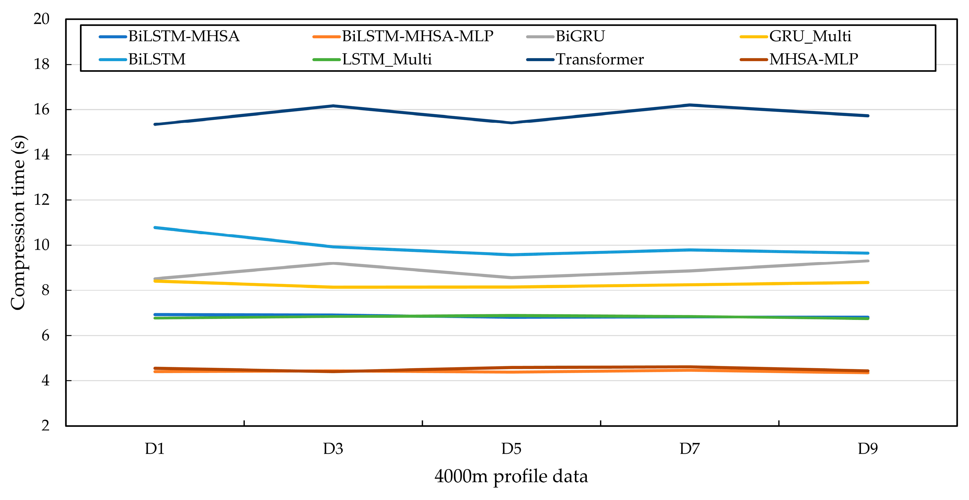
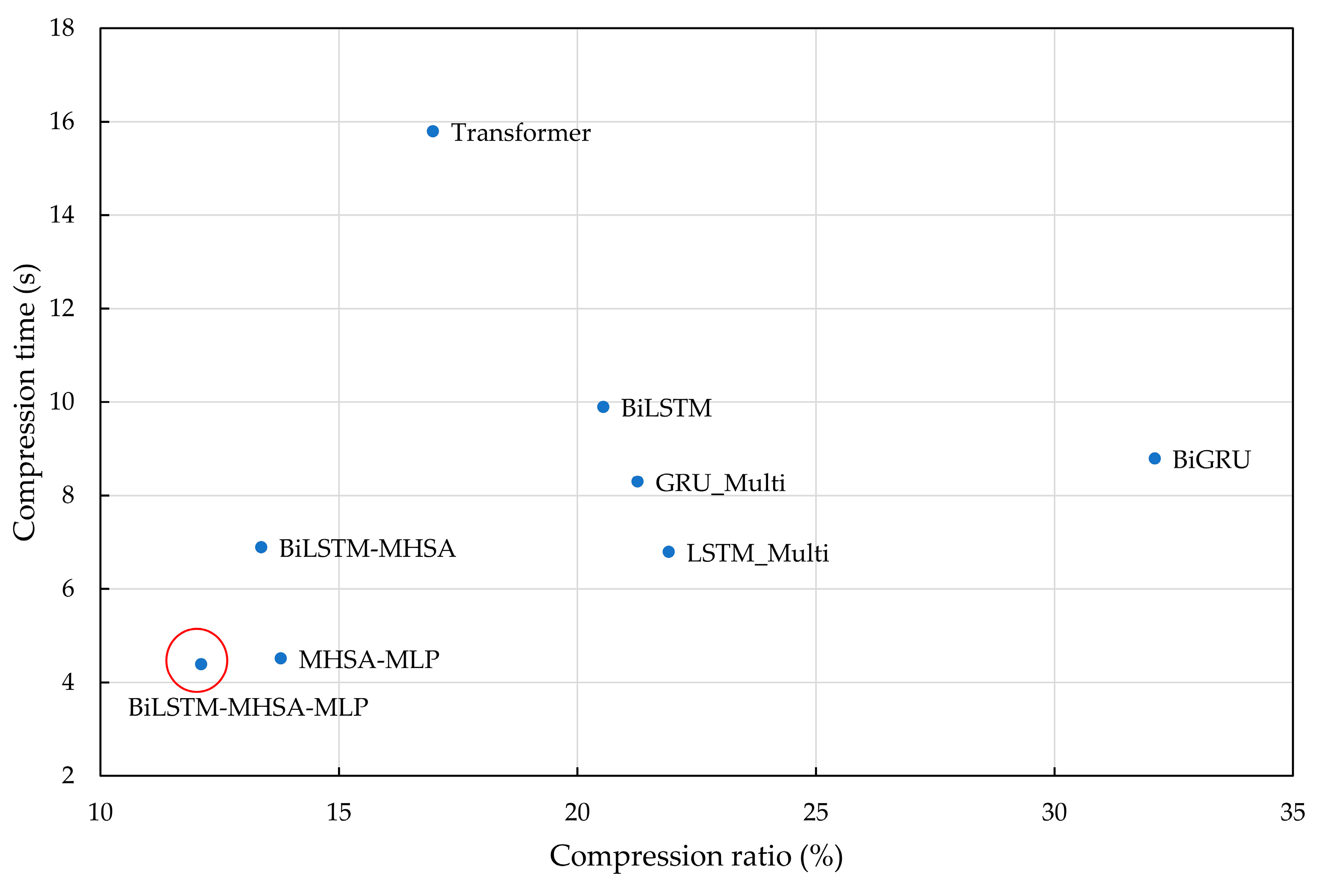
Second, the compression algorithm in this paper is compared with traditional deep learning compression algorithms (BiGRU, GRU_Multi, BiLSTM, LSTM_Multi, Transformer, and MHSA-MLP). The probability prediction model is obtained through the abovementioned deep learning algorithm, and then combined with arithmetic coding to achieve lossless compression. Among them, MHSA-MLP adopts multi-head self-attention combined with absolute position encoding as the preliminary probability prediction model, and it introduces an MLP to realize block compression while training, which is in contrast to the preliminary probability prediction model (BiLSTM-MHSA) and the probability prediction model (BiLSTM-MHSA-MLP) presented in this paper. The compression ratio and compression time are shown in Figure 15 and Figure 16.

The average compression ratios of the traditional deep learning compression algorithms (BiGRU, GRU_Multi, BiLSTM, LSTM_Multi, Transformer, and MHSA-MLP) are 32.1%, 21.26%, 20.54%, 21.91%, 16.97%, and 13.78%, respectively, and the average compression times are 8.8 s, 8.3 s, 9.9 s, 6.8 s, 15.8 s, and 4.5 s, respectively. Compared with traditional compression algorithms, the average compression ratio is significantly lower, indicating that deep learning compression algorithms are superior to traditional compression algorithms. Compared with MHSA-MLP, the compression algorithm in this paper reduces the average compression ratio by 1.67%, and the average compression time is almost the same. This shows that introducing the BiLSTM layer before the MHSA layer can provide richer context information and improve the model’s modeling ability for profile data. In addition, compared with the traditional deep learning compression algorithm, the compression algorithm in this paper reduces the average compression ratio by 10.45% and the average compression time by 5.5 s. This shows that the compression algorithm in this paper has better performance. Compared with those of the previous four RNN algorithms, the compression ratio of the Transformer algorithm is lower, but the compression time is increased.

Compared to traditional deep learning compression algorithms, the proposed compression algorithm is more suitable for Argo buoy profile data. Argo buoy data exhibits clear time-series characteristics and temporal dependencies, which BiLSTM can effectively capture by processing the input sequence in both directions, helping to analyze and compress the temporal patterns within the data. The MHSA layer further enhances the processing of relationships between different parts of the data by focusing on key time steps, thereby capturing richer contextual information and improving compression performance. The MLP optimizes the compression process by dynamically adjusting the strategy, enhancing compression efficiency. Therefore, BiLSTM-MHSA-MLP is more advantageous than traditional algorithms in handling buoy data with temporal dependencies and dynamic variations.

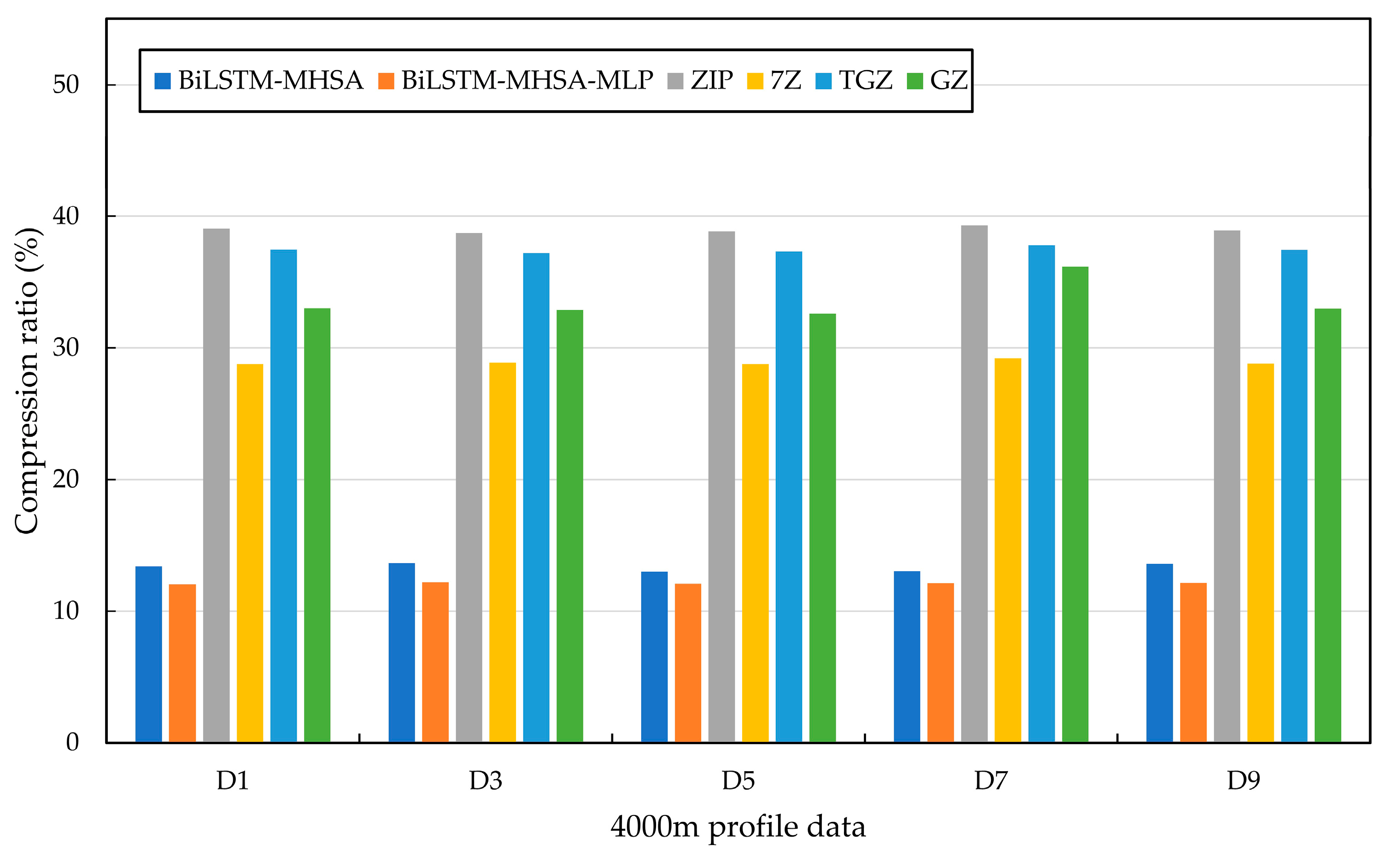
Finally, the compression algorithm in this paper is compared with popular compressors (ZIP, 7Z, TGZ, and GZ), and the compression ratio results are shown in Figure 17.

As shown in Figure 17, the performance of the compression algorithm in this paper is significantly better than that of popular compressors. The average compression ratios of the four compressors are 38.96%, 28.88%, 37.45%, and 33.55%, all with compression times of less than 1 s. Compared to the proposed algorithm, the average compression ratio is improved by 22.6%. This indicates that the proposed compression algorithm is more targeted and demonstrates better performance in compressing 4000 m profile Argo buoy data.

4.5. Discussion

In summary, the compression algorithm proposed in this paper outperforms traditional compression algorithms (Huffman, LZW, PPM, Bzip2, and Mtfpc), traditional deep learning compression algorithms (BiGRU, GRU_Multi, BiLSTM, LSTM_Multi, Transformer, and MHSA-MLP), as well as popular compressors (ZIP, 7Z, TGZ, and GZ) in terms of both compression ratio and compression time.

Table 4. Comparison of the effects of different compression algorithms.

Compression Algorithm	Average Compression Ratio (%)	Average Compression Time (s)
Traditional compression algorithms	46.25	<1
Traditional deep learning compression algorithms	22.56	9.9
Popular compressors	34.71	<1
This article (PC)	12.11	4.4
This article (Jetson nano)	12.11	36.6

presents the average compression ratio and average compression time. To evaluate compression performance, this study uses compression ratio and compression time as the primary statistical indicators. Compression time represents the computational time required for the data compression process, while compression ratio measures the proportion of the compressed data size to the original data size. A smaller compression ratio indicates better compression performance. The calculation of the compression ratio is expressed by Equation (9). In this context, compressed data size represents the size of the compressed data, and original data size represents the size of the original data.

$$\mathrm{compression} \mathrm{ratio}={\displaystyle \frac{\mathrm{compressed} \mathrm{data} \mathrm{size}}{\mathrm{original} \mathrm{data} \mathrm{size}}}$$

(9)

Among them, the average compression time for traditional compression algorithms and popular compressors is less than 1 s, with average compression ratios of 46.25% and 34.71%, respectively. The compression ratios are 30.14% and 22.6% higher than the compression algorithm proposed in this paper, respectively. Although the average compression time is relatively short, the average compression ratio is relatively high, resulting in unsatisfactory compression performance overall. The average compression time of traditional deep learning compression algorithms is approximately 9 s longer than that of traditional compression algorithms and popular compressors. However, the average compression ratio is reduced by 23.69% and 12.15%, respectively. The comparison between the proposed compression algorithm and traditional deep learning compression algorithms on the PC is shown in Figure 18. Compared to traditional deep learning compression algorithms, the proposed compression algorithm not only achieves a lower compression ratio but also shorter compression time. Additionally, in comparison with the three baseline methods, the p-value between compression ratios was introduced as a statistical significance test metric. In this study, the p-value is used to determine whether the proposed compression method exhibits a significant difference in compression performance compared to the baseline methods. The results show that the p-values for the proposed compression algorithm compared to the three baseline methods are all less than 0.05, indicating that the statistical tests reveal a significant difference in compression performance. Further analysis demonstrates that the proposed compression algorithm significantly outperforms these three baseline methods in terms of compression effectiveness.

Specifically, the compression algorithm achieves an average compression ratio of 12.11% on both the PC and Jetson Nano, with an average compression time of 4.4 s on the PC and 36.6 s on the Jetson Nano. Compared to the first three methods, the proposed algorithm reduces the average compression ratio by 34.14%, 10.45%, and 22.6%, respectively, achieving a significant decrease in compression ratio. The average compression time on the PC is reduced by 5.5 s compared to traditional deep learning compression algorithms, while the average compression time on the Jetson Nano is increased by 32.2 s compared to the PC. Although the compression time on the Jetson Nano is relatively longer, it is acceptable for the data transmission of the Argo buoy. The Argo buoy’s main control board sends profile data to the satellite every 65 s, with each transmission consisting of 228 bytes of data. For example, in the case of 4000 m Data 1, uncompressed data requires a total of 4486 bytes to be transmitted, taking approximately 1300 s with 20 transmissions. The energy consumption per transmission is about 151 J, resulting in a total energy consumption of approximately 3020 J. After compression using the Jetson Nano platform, the data size is reduced to 540 bytes, the transmission time is shortened to 195 s, and the number of transmissions is reduced to 3. During the deep learning-based compression task, the Jetson Nano consumes an average of 8.5 W and completes the task in about 37 s, requiring 315 J of energy. With data compression, the total energy consumption for transmitting one profile is reduced to 453 J, significantly lower than the 3020 J required without compression. Overall, data compression reduces the total energy consumption used for transmitting a single batch of profile data to 768 J, saving approximately 2252 J compared to the uncompressed scenario. This not only significantly shortens the data transmission time between the Argo float and the satellite but also effectively reduces energy consumption.

Although the compression algorithm proposed in this paper achieves significant results compared to the three baseline methods, it still has certain limitations. The algorithm is primarily designed for single-batch profile data from Argo floats and builds the alphabet through character matching. Specifically, the data to be compressed must conform to a specific alphabet; if the data contains characters not in the alphabet, the algorithm will fail to operate correctly and will report an error. Furthermore, the algorithm may not be applicable to other types of data, such as those collected by the Argo float’s hydrophone, which limits its effectiveness in broader applications.

5. Conclusions

Faced with the limited storage capacity of the Argo buoy’s SD card and the fact that satellite communications are generally charged by data volume, this paper proposes a block-based lossless data compression method based on a BiLSTM-MHSA-MLP, and it transplants the algorithm from the PC to the Jetson nano development board to achieve lossless data compression. The preliminary probability prediction model in this paper is constructed mainly via the BiLSTM and the MHSA, which pay more attention to the correlations among profile data, learn the relationships and characteristics of the data in parallel, and improve the generalization ability of the probability prediction model and its ability to capture complex patterns. On this basis, MLP and block_len are introduced to realize block compression while training. The model can dynamically update the probability model during the compression process, gradually adapting to the distribution of compressed data, and thus providing more accurate probability predictions.

Compared with traditional mainstream compression algorithms, the compression method in this paper has a lower compression ratio and shorter compression time, and it is more suitable for Argo buoys. In addition, the compression algorithm in this paper was transplanted to the Jetson nano development board and lossless compression was achieved. The Argo buoy first sends the collected profile data to the Jetson nano development board through the serial port for compression, and then uses the compressed profile data for satellite communication, which can greatly reduce the time and communication cost of data transmission between the buoy and the satellite. It also lays the foundation for the subsequent transplantation of the Jetson nano development board to the Argo buoy to achieve real-time data compression.

Currently, the model is primarily trained using profile data, but due to the limitations of the data type, its application scope is somewhat restricted. To broaden the model’s application, we plan to introduce other types of Argo float data in the future, such as hydrophone data, to enhance the model’s generalization ability and applicability. Furthermore, the current model is based on a complex deep learning architecture, resulting in high computational complexity, which may lead to inference speed bottlenecks. Therefore, we will consider using optimization tools such as TensorRT to accelerate the model, significantly improving the inference efficiency for data compression tasks. Additionally, techniques like quantization and pruning will be employed to further optimize inference speed and reduce power consumption. Furthermore, to ensure the efficiency and reliability of data transmission between the Jetson Nano and the main control board, the communication protocol needs to be improved in the future, to enhance the data transmission and verification mechanisms. This would help ensure data integrity and accuracy, thus improving the overall system performance and reliability.