Bearing-Only Multi-Target Localization Incorporating Waveguide Characteristics for Low Detection Rate Scenarios in Shallow Water

Abstract

Bearing-only multi-target localization (BOMTL) determines the positions of multiple targets by intersecting bearing lines from multiple spatial locations. However, non-ideal measurements can result in a large number of ghost targets. A β-S-dimensional assignment (β-SDA) method incorporating waveguide characteristics is proposed to address the BOMTL problem in shallow water with low detection rates. The estimated distance for the warping transformation is derived from the intersection points of the bearing lines, then the autocorrelation function of the broadband beamforming output is transformed using a warping operator to obtain the corresponding characteristic spectrum. The peaks in the characteristic spectrum correspond to the cross-correlation terms of the normal modes, with the frequencies of these peaks related to the ratio of the actual distance to the estimated distance of the sound source. The global target localization results are obtained using the proposed method, which incorporates confidence coefficients derived from the characteristic spectrum and geometric intersection information from the bearing lines. Simulation and sea trial data demonstrate that the β-SDA method effectively overcomes the limitation of pure bearing-only localization in low detection rate scenarios under a given signal-to-noise ratio (SNR), and can localize target positions without requiring precise prior environmental parameters.

1. Introduction

Bearing-only Target Localization (BOTL) has broad applications in fields such as communication [1], radar [2,3], and sonar [4,5], where it estimates target positions using bearing angle information from multiple spatially distributed sensors. In the case of multiple arrays and multiple targets, the intersection point corresponding to each target is unique when there are no measurement errors, the detection rate is 1, and no spurious measurements are present. Moreover, the number of bearing lines forming the intersection point equals the number of arrays. However, in underwater acoustic measurement environments, the bearing angles are affected by measurement errors and low detection rates, leading to a large number of ghost targets. The solution to the BOMTL problem is typically divided into two steps: (1) data association [6,7,8], which involves clustering measurements from the same target; (2) target position estimation [9,10,11], where measurements belonging to the same target are used to estimate the positions of the targets.

In the BOMTL problem, the assumption of a one-to-one correspondence between the targets and the bearing lines renders the data association problem NP-hard when the number of arrays is three or more [12]. Furthermore, the arctangent relationship between the measurements and the target states introduces substantial nonlinearity into the system [13]. The primary challenge in multi-target scenarios is the data association. Bar-Shalom et al. first developed a data association model for multiple passive sensors and performed a multi-dimensional data assignment using a cost function based on various combinations [14]. Building on this association model, researchers have proposed several methods to address the data association challenge in the BOMTL problem. Based on the geometric distances, ghost targets are excluded using a method inspired by K-means clustering [15]. The algorithm has low complexity and is easy to implement; however, it requires high measurement accuracy and shows low association accuracy in complex environments. Based on the spectral characteristics of radiation sources, the measured periodic frequency is matched with each radiation source to establish the association [16]. This approach requires prior knowledge of the periodic frequency of each radiation source. However, in practical applications, this method is constrained by the need for prior knowledge of the radiation sources and measurement conditions, which may lead to potential shortcomings. In addition, parameters reflecting the motion characteristics of the source can also be extracted from the measurements [17], thereby enhancing the accuracy of the association. From the perspective of the maximum likelihood method [18], a measurement model is established to compute the likelihood function for each possible combination. The assignment is then derived from all possible combinations. While this method achieves high association accuracy in complex environments, its computational complexity grows exponentially with the number of targets and measurements, rendering it impractical for real-time processing. To enhance its practicality, Lagrangian relaxation techniques are applied to the assignment method [19]. The S-dimensional assignment (SDA) algorithm [20] constructs an association cost matrix and employs a recursive continuous Lagrangian relaxation operator to obtain an optimal or suboptimal solution that satisfies the constraints, thereby providing strong real-time performance and scalability. In general, research on optimizing data association performance focuses primarily on two aspects: (1) optimizing the cost function for various application scenarios to enhance the method’s stability and accuracy; (2) using prior knowledge or constraints to reduce the dimensionality of all possible association combinations [21], which not only improves computational speed but also mitigates interference from redundant association combinations, thereby enhancing association accuracy. Once data association is completed, the multi-array, multi-target bearing-only localization problem is reduced to several multi-array, single-target bearing-only localization problems.

Most localization methods for the BOMTL problem estimate target positions based on the geometric intersection information of the bearing lines within the surveillance area. However, it faces inherent limitations at low detection rates, particularly when the number of bearing lines corresponding to ghost targets is greater than or equal to that corresponding to real targets, which makes accurate data association and localization challenging. The shallow water waveguide introduces significant modal characteristics in the received signals, offering a novel approach to addressing the BOMTL problem.

The β-S-dimensional assignment (β-SDA) method is proposed as a solution to the aforementioned challenge. The waveguide invariant β demonstrates that the method exploits the invariance of the waveguide. The estimated distance for the warping transformation is derived from the intersection points. A warping transformation [22,23] is then applied to the autocorrelation function of the beamforming output signal to extract the cross-correlation terms of the normal modes. The frequencies of the peaks in the transformed characteristic spectrum are related to the actual and the estimated distances to the target. The correlation coefficients between the characteristic spectra of different bearing lines are then computed. The feasibility and limitations of using the correlation coefficients to assess the authenticity of the intersection points are analyzed through derivation and simulation. A likelihood function that incorporates both waveguide characteristics and geometric information is established, and global target position estimates are obtained using the SDA algorithm. The proposed β-SDA method optimizes the traditional association cost function by incorporating waveguide characteristics, thereby improving the accuracy of bearing-only multi-target localization using multiple arrays in shallow water environments with low detection rates.

2. Theoretical Development

2.1. Extraction of the Characteristic Spectrum from Beamforming Output Signals

According to the theory of normal mode, in a horizontally invariant waveguide, the received signals from a horizontal linear array (HLA) characterized by an inter-element spacing of d and an element count of N can be expressed as follows:

$$p_n(f)=S(f){\displaystyle \sum _{m=1}^M{A}_m(f)\exp [{\mathrm{ik}}_m(f)}{r}_n],$$

(1)

$$A_m(f)={\displaystyle \frac{\mathrm{i}\exp (-\mathrm{i}\pi /4)}{\rho (z_s)\sqrt{8\pi r_n}}}{\displaystyle \frac{{\psi }_m(z_s){\psi }_m(z)}{\sqrt{k_m(f)}}},$$

(2)

where $S(f)$ denotes the source spectrum, $z_s$ and $z$ denote the depths of the source and the receiving point, respectively. ${\psi }_m$ is the eigenfunction of the m-th mode, and $k_m$ is the horizontal wavenumber of the m-th mode. $r_n$ is the distance between the source and the n-th hydrophone.

The azimuth of the source relative to the broadside of the array is denoted by ${\theta }_T$. Under the assumption of far-field conditions, $r_n$ can be expressed as follows: $r_n\approx r_0-(n-1)d\sin ({\theta }_T)$, where $r_0$ is the distance from the sound source to the reference hydrophone.

The frequency domain expression of the autocorrelation function of the broadband beamforming output, along the direction of the incoming wave from the source, is given as follows:

$$B({\theta }_T,f)={\left|{\displaystyle \sum _{n=1}^N\exp [\mathrm{i}(n-1)k_{0}d\sin ({\theta }_T)]p_n(f,r_n)}\right|}^2,$$

(3)

where $k_0=2\pi f/c_0$, $c_0$ denotes the reference sound speed. Substituting Equation (1) into Equation (3) yields the following results:

$$\begin{array}{c}B({\theta }_T,f)={\left|S(f)\right|}^2{\left|{\displaystyle \sum _{m=1}^M{A}_m\exp (\mathrm{i}{k}_m{r}_T)\mathrm{sinb}({\Delta }_m)}\right|}^2\\ ={\left|S(f)\right|}^2\{{\displaystyle \sum _{m=1}^M{\left|A_m\mathrm{sinb}({\Delta }_m)\right|}^2+{\displaystyle \sum _{m\ne n}{A}_m{A}_n^{\ast }\exp [\mathrm{i}(k_m-k_n)r_T]\mathrm{sinb}(}}{\Delta }_m)\mathrm{sinb}({\Delta }_n)\},\end{array}$$

(4)

where:

$$r_T=r_0-{\displaystyle \frac{N-1}{2}}d\sin ({\theta }_T),$$

(5)

$${\Delta }_m=k_0\sin ({\theta }_T)-k_m\sin ({\theta }_T),$$

(6)

$$\mathrm{sinb}(x)={\displaystyle \frac{\sin (Ndx/2)}{\sin (dx/2)}}.$$

(7)

Assuming that ${\Delta }_m$ approaches 0 [24], we obtain $\mathrm{sinb}({\Delta }_m)\approx N$. Equation (4) simplifies to:

$$B({\theta }_T,f)=N^2{\left|S(f)\right|}^2\{{\displaystyle \sum _{m=1}^M{\left|A_m\right|}^2+{\displaystyle \sum _{m\ne n}{A}_m{A}_n^{\ast }\exp [\mathrm{i}(k_m-k_n)r_T]}}\}.$$

(8)

The maximum value of the autocorrelation function, as described in Equation (8), is set to the zero point. Only the positive half of the zero point is considered, and values near the zero point are set to zero to eliminate the autocorrelation component of the normal modes. The remaining cross-correlation component of the normal modes is given by:

$$B({\theta }_T,f)={\displaystyle \sum _{l=1}^L{D}_l\exp (\mathrm{i}{k}_l{r}_T)},$$

(9)

where $D_l=N^2{\left|S(f)\right|}^2{A}_m{A}_n^{\ast }$ and $k_l=k_m-k_n$. $L=C_M^2$ is the number of pairwise combinations of $M$ normal modes. When the estimated distance to the sound source is $\widehat{r}$, $B({\theta }_T,f,\widehat{r})$ is obtained by applying a phase shift to $B({\theta }_T,f)$:

$$B({\theta }_T,f,\widehat{r})={\displaystyle \sum _{l=1}^L{D}_l\exp (\mathrm{i}{k}_l{r}_T)}\exp (-\mathrm{i}2\pi f{t}_{\widehat{r}}),$$

(10)

where $t_{\widehat{r}}=\widehat{r}/c_0$.

For an ideal waveguide, when the cutoff frequency of the m-th normal mode satisfies $f_m\ll f$, the Taylor series approximation is given by:

$$k_l\approx {\displaystyle \frac{2\pi }{c_0}}({\displaystyle \frac{f_n^2}{2f}}-{\displaystyle \frac{f_m^2}{2f}}),$$

(11)

Substituting Equation (11) into Equation (10) yields:

$$B({\theta }_T,f,\widehat{r})\approx {\displaystyle \sum _{l=1}^L{D}_l\exp [-\mathrm{i}2\pi t_{\widehat{r}}\sqrt{f^2-{\left(\sqrt{\frac{r_T}{\widehat{r}}}{\mu }_l\right)}^2}]},$$

(12)

where ${\mu }_l=\sqrt{f_n^2-f_m^2}$. Assuming that the amplitude spectrum of the sound source varies slowly, the inverse Fourier transform of Equation (12) can be evaluated using the stationary phase method [25] as:

$$R(t,r_T,\widehat{r})={\displaystyle \sum _{l=1}^L{D}_l(\sqrt{\frac{r_T}{\widehat{r}}}{\mu }_{l}t{(t^2-t_{\widehat{r}}^2)}^{-\frac{1}{2}})t_{\widehat{r}}{(\sqrt{\frac{r_T}{\widehat{r}}}{\mu }_l)}^{\frac{1}{2}}}{\displaystyle \frac{\sqrt{2}}{2}}{(t^2-t_{\widehat{r}}^2)}^{-{\displaystyle \frac{3}{4}}}\exp (\mathrm{i}2\pi \sqrt{{\displaystyle \frac{r_T}{\widehat{r}}}}{\mu }_l\sqrt{t-t_{\widehat{r}}^2}).$$

(13)

Using the warping operator $h(t)=\sqrt{t^2+t_{\widehat{r}}^2}$ to resample Equation (13) yields:

$$W_{h}R(t,r_T,\widehat{r})={\left|{\displaystyle \frac{\partial h(t)}{\partial t}}\right|}^{{\displaystyle \frac{1}{2}}}{\displaystyle \sum _{l=1}^L{D}_l(\sqrt{\frac{r_T}{\widehat{r}}}{\mu }_l\sqrt{t+t_{\widehat{r}}^2}/t)t_{\widehat{r}}{(\sqrt{\frac{r_T}{\widehat{r}}}{\mu }_l)}^{\frac{1}{2}}\frac{\sqrt{2}}{2}}{t}^{-{\displaystyle \frac{3}{2}}}\exp (\mathrm{i}2\pi \sqrt{{\displaystyle \frac{r_T}{\widehat{r}}}}{\mu }_{l}t).$$

(14)

The spectrum obtained from the Fourier transform of Equation (14) is referred to as the characteristic spectrum when the source has an azimuth of ${\theta }_T$ and an estimated distance of $\widehat{r}$. The characteristic spectrum exhibits peaks at the characteristic frequencies $\sqrt{r_T/\widehat{r}}{\mu }_l$. When $\widehat{r}=r_T$, the characteristic frequency is determined by the cutoff frequencies of the various normal modes, which reflect the waveguide characteristics. Therefore, when the intersection points correspond to real targets, the characteristic spectra of the bearing lines that define them exhibit the same characteristic frequencies.

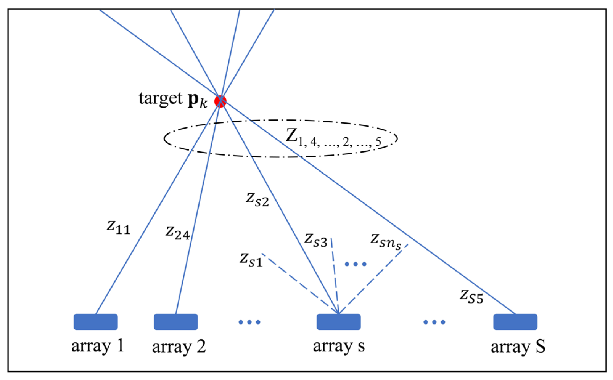
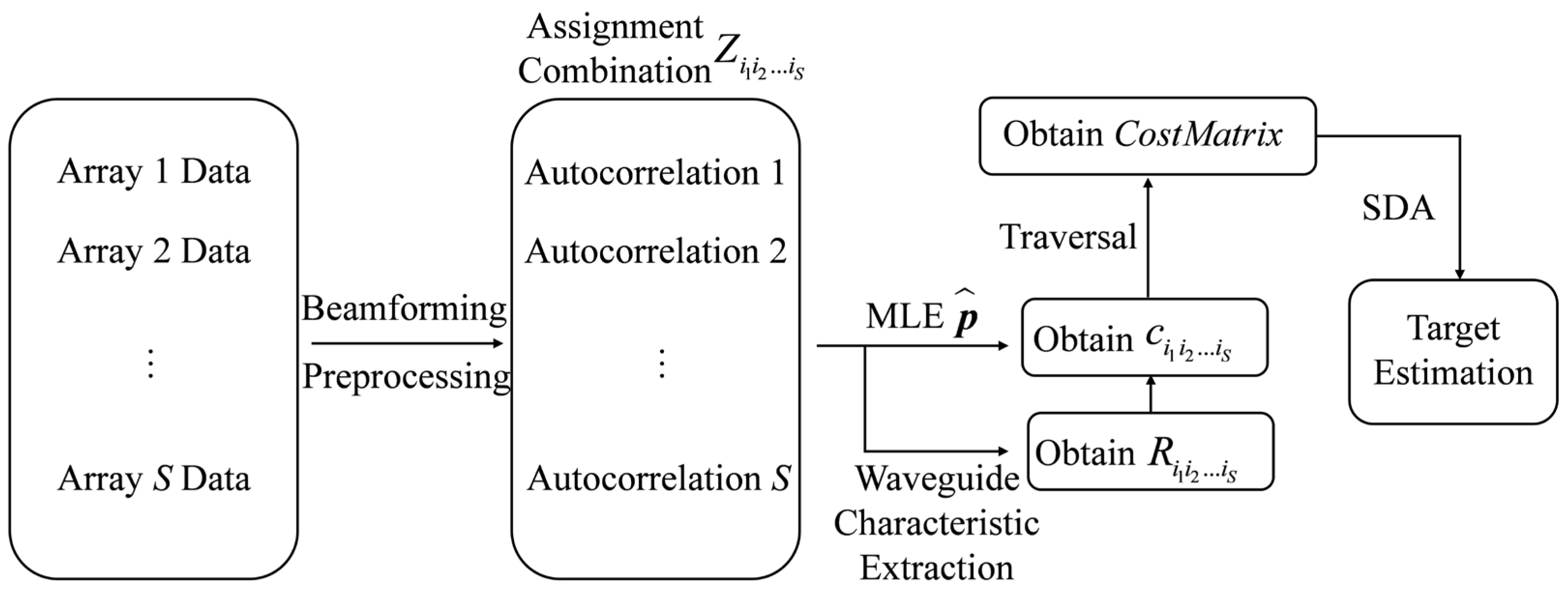
2.2. Localization Incorporating Waveguide Characteristics

The two-dimensional bearing-only multi-target localization problem can be formulated as follows: There are $S$ arrays and $K$ targets within the surveillance area. The coordinates of the targets are denoted as $p_k=(x_k,y_k), k=1,\dots ,K$, and the reference coordinates of the arrays are denoted as $p_s=(x_s,y_s), s=1,\dots ,S$. The ideal measurement corresponding to target $p_k$, as output by array $p_s$, can be expressed as:

$$H(p_k,p_s)=\arctan ({\displaystyle \frac{y_k-y_s}{x_k-x_s}}).$$

(15)

The measurement set out by a given array is denoted as $z_{s{i}_s}$, where $s=1,2\dots S$ corresponds to the array index and $i_s=0,1,\dots ,n_s$ corresponds to the measurement index output by array s. If $i_s=0$, it indicates that the array s has no measurement corresponding to the targets. A combination of measurements selected from each array is denoted as $Z_{i_1{i}_2\dots i_S}$. The schematic diagram of the two-dimensional bearing-only multi-target localization model is shown in Figure 1.

The following assumptions are made:

• When the measurement is originated from target $p_k$, the measurement $z_{s{i}_s}$ can be represented as $z_{s{i}_s}=H(p_k,p_s)+{ϵ}_s$, where ${ϵ}_s~\mathcal{N}(0,{\sigma }_s^2)$ is white Gaussian noise;
• When the measurement originated from a spurious source, the measurement $z_{s{i}_s}$ is uniformly distributed within the array’s surveillance area;
• Each target satisfies the observability condition [26], and the positional change of the target during a single measurement interval is negligible.

Under the aforementioned assumptions, each association combination $Z_{i_1{i}_2\dots i_S}$ is associated with a corresponding association cost $c_{i_1{i}_2\dots i_S}$. All possible combinations of associations form the association cost matrix $C\in {ℝ}^{(n_1+1)\times (n_2+1)\times \dots \times (n_S+1)}$.

The nomenclature is shown in

Table 1. Nomenclature.

$N_{\mathrm{inter}}$	Number of valid intersection points
$z_{s_1{i}_{s_1}}$, $z_{s_2{i}_{s_2}}$	Measurements from arrays $s_1$ and $s_2$
${\theta }_{i_{s_1}}$, ${\theta }_{i_{s2}}$	Azimuths of $z_{s_1{i}_{s_1}}$ and $z_{s_2{i}_{s_2}}$
$B_{s_1}({\theta }_{i_{s_1}},f)$, $B_{s_2}({\theta }_{i_{s_2}},f)$	Frequency domain outputs of beamformers
$R_{s_1}({\theta }_{i_{s_1}},t)$, $R_{s_2}({\theta }_{i_{s_2}},t)$	Time domain autocorrelation functions
$r_{s_1}$, $r_{s_2}$	Distances from the intersection point to arrays
$P_{D_s}$	Detection rate of the array s
$u(i_s)$	Indicator function
${\mathsf{\Psi }}_s$	Field of view of array s
$R_{i_1{i}_2\dots i_S}$	Confidence coefficient for combination $Z_{i_1{i}_2\dots i_S}$
$\mathsf{\Lambda }(Z_{i_1{i}_2\dots i_S}|p_k)$	Likelihood function for combination $Z_{i_1{i}_2\dots i_S}$
$c_{i_1{i}_2\dots i_S}$	Association cost for combination $Z_{i_1{i}_2\dots i_S}$

. The cost function, incorporating waveguide characteristics, can be obtained as follows:

• Set the values near the maximum of the autocorrelation function to zero, and shift it to the right by $t_{s_1}={r_{s_1}/c}_0$ and $t_{s_2}={r_{s_2}/c}_0$ to obtain ${\tilde{R}}_{s_1}({\theta }_{i_{s_1}},t-t_{s_1})$ and ${\tilde{R}}_{s_2}({\theta }_{i_{s_2}},t-t_{s_2})$, where $c_0$ is the reference sound speed;
• Apply the warping operator $h_{s_1}(t)=\sqrt{t^2+t_{s_1}^2}$ and $h_{s_2}(t)=\sqrt{t^2+t_{s_2}^2}$ to resample ${\tilde{R}}_{s_1}$ and ${\tilde{R}}_{s_2}$. Subsequently, perform a Fourier transform to obtain the characteristics spectra $F_{s_1}({\theta }_{i_{s_1}},f)$ and $F_{s_2}({\theta }_{i_{s_2}},f)$. The correlation coefficient is given by:

  $$R_F={\displaystyle \frac{{\displaystyle {\int }_{f_1}^{f_2}[\left|F_{s_1}({\theta }_{i_{s_1}},f)\right|-\overline{\left|F_{s_1}({\theta }_{i_{s_1}},f)\right|}][\left|F_{s_2}({\theta }_{i_{s_2}},f)\right|-\overline{\left|F_{s_2}({\theta }_{i_{s_2}},f)\right|}]}df}{\sqrt{{\displaystyle {\int }_{f_1}^{f_2}{[\left|F_{s_1}({\theta }_{i_{s_1}},f)\right|-\overline{\left|F_{s_1}({\theta }_{i_{s_1}},f)\right|}]}^{2}df{\displaystyle {\int }_{f_1}^{f_2}{[\left|F_{s_2}({\theta }_{i_{s_2}},f)\right|-\overline{\left|F_{s_2}({\theta }_{i_{s_2}},f)\right|}]}^{2}df}}}}},$$

  (16)

  where $f_1$ and $f_2$ represent the selected frequency ranges of the characteristic spectra. The confidence coefficient is expressed as: $R_{i_1{i}_2\dots i_S}={\displaystyle \sum _{n_{\mathrm{inter}}=1}^{N_{\mathrm{inter}}}{R}_{F,n_{\mathrm{inter}}}}.$
• The likelihood function is expressed as follows:

  $$\mathsf{\Lambda }(Z_{i_1{i}_2\dots i_S}|p_k)={\displaystyle \prod _{s=1}^S{(1-P_{D_s})}^{1-u(i_s)}{[P_{D_s}{R}_{i_1{i}_2\dots i_S}p(z_{{\mathit{si}}_{\mathit{s}}}|p_k)]}^{u(i_s)}},$$

  (17)

  where $u(i_s)$ is given by:

  $$u(i_s)=\left\{\begin{array}{l}0\hspace{1em}{i}_s=0\\ 1\hspace{1em}{i}_s\ne 0\end{array}\right..$$

  (18)

The actual target position $p_k$ is replaced by the maximum likelihood estimate $\widehat{p_k}=\arg \underset{p_k}{\max }\tilde{\mathsf{\Lambda }}(Z_{i_1{i}_2\dots i_S}|p_k)$, where:

$$\tilde{\mathsf{\Lambda }}(Z_{i_1{i}_2\dots i_S}|p_k)={\displaystyle \prod _{s=1}^S{(1-P_{D_s})}^{1-u(i_s)}{[P_{D_s}p(z_{{\mathit{is}}_s}|p_k)]}^{u(i_s)}}.$$

(19)

Under the given assumption, the likelihood function, assuming that none of the measurements originate from target $p_k$, is expressed as follows:

$$\mathsf{\Lambda }(Z_{i_1{i}_2\dots i_S}|p_k=\varnothing )={\displaystyle \prod _{s=1}^S{(\frac{1}{{\mathsf{\Psi }}_s})}^{u(i_s)}},$$

(20)

The association cost can be expressed using the likelihood ratio function as follows:

$$c_{i_1{i}_2\dots i_S}=-\ln [{\displaystyle \frac{\mathsf{\Lambda }(Z_{i_1{i}_2\dots i_S}|p_k)}{\mathsf{\Lambda }(Z_{i_1{i}_2\dots i_S}|p_k=\varnothing )}}].$$

(21)

After obtaining the association cost matrix, which incorporates waveguide characteristics, data association and localization can be performed using the SDA method. The entire process of the proposed β-SDA method is illustrated in a block diagram shown in Figure 2.

3. Numerical Simulations and Experimental Validation

In this section, the properties of the characteristic spectrum are first analyzed using both theoretical analysis and simulations. Subsequently, the localization performance of the β-SDA method is evaluated under various detection rates and signal-to-noise ratios (SNRs), with a focus on the correct localization rate (CLR) and false localization rate (FLR). Finally, sea trial data are processed to assess the practical applicability of the proposed method.

3.1. Analysis of the Characteristic Spectrum

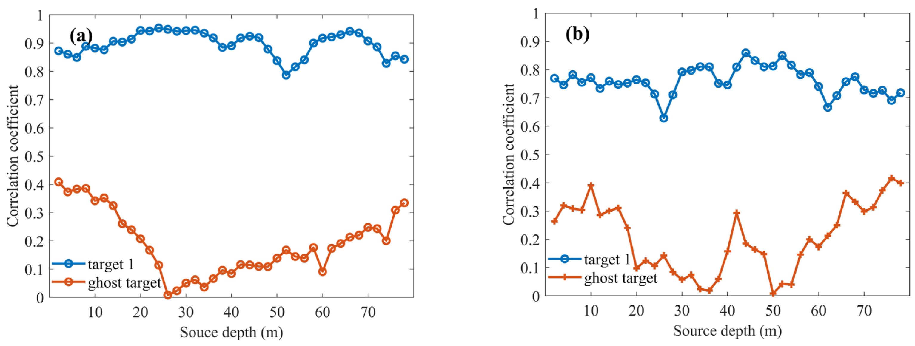
3.1.1. Properties of the Correlation Coefficient

For simplicity, the properties of the characteristic spectrum corresponding to the two HLAs are analyzed. The sound field is calculated using KRAKENC (https://oalib-acoustics.org/models-and-software/acoustics-toolbox/, accessed on 1 December 2024) [27]. Two identical HLAs, each consisting of 100 equidistantly spaced hydrophones and spanning a length of 198 m, are deployed on the seabed. The reference coordinates of the HLAs are (0 km, 0 km) and (20 km, 0 km), respectively. The endfire direction is aligned along the x-axis. The positions of the two targets are (8 km, 20 km) and (18 km, 15 km), both at a depth of 20 m. The frequency range of the received broadband signal is from 50 Hz to 150 Hz, and the averaged received SNR for a single hydrophone in the frequency domain is −5 dB. The warping derived from the ideal waveguide is a robust transformation, which is applicable to most low-frequency shallow water environments [28]. The water depth is 80 m, and the sound speed profile is shown in Figure 3. The bottom attenuation coefficient is $0.517f^{1.07}\mathrm{dB}/\lambda$ (the unit of f is kHZ) [29].

The beamforming outputs of HLA 1 and HLA 2 are shown in Figure 4. The intersections of the output bearing lines are presented in Figure 5, where HLA 1 detects both targets and HLA 2 detects only target 1.

Due to the significant attenuation of higher-order normal modes during long-distance propagation, the characteristic frequencies ${\mu }_l$ corresponding to the cross-correlation terms between lower-order normal modes are relatively small. Consequently, the frequency range for the integration of the characteristic spectra is selected from 0 Hz to 50 Hz. The characteristics spectra corresponding to target 1, obtained from the simulated received signal, are shown in Figure 6. The correlation coefficient is 0.91, and the three peaks correspond to the cross-correlation terms of the (1, 2), (2, 3), and (1, 3) normal modes, respectively. In total, 100 Monte Carlo trials are conducted at each SNR to obtain the correlation coefficient for target 1 and ghost target, with the average received SNR ranging from −15 dB to 0 dB, as shown in Figure 7.

The correlation coefficient is high when the intersection point corresponds to a true target, as the characteristic frequencies align (see Figure 6). However, the performance in extracting the cross-correlation terms of normal modes deteriorates as the SNR decreases (see Figure 7).

While the correlation coefficient of the characteristic spectra can indicate the authenticity of the intersection points, it is influenced by several factors: (1) The correlation coefficient is affected by SNR. (2) The estimated distances $\widehat{r_1}$ and $\widehat{r_2}$ that satisfy $\sqrt{r_1/{\widehat{r}}_1}{\mu }_l=\sqrt{r_2/{\widehat{r}}_2}{\mu }_l$ are not unique. Although this situation is rare, it may lead to a ghost target corresponding to falsely high correlation coefficients. In multi-array, multi-target scenarios, the complexity of bearing line intersections further complicates the data association process. Therefore, it is essential to incorporate both the waveguide characteristics and the geometric information of the bearing lines to enhance the accuracy and stability of the localization method.

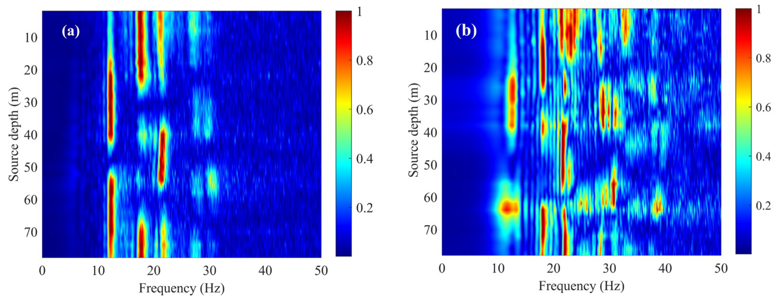
3.1.2. Effect of Source Frequency and Depth

Section 3.1.1 evaluates the feasibility of employing the correlation coefficient to assess the authenticity of intersection points within a specific frequency band and depth. The number of modes, as well as the amplitude of each mode, are influenced by the source frequency, and depth. Therefore, both the source frequency and depth can alter the number, frequency, and amplitude of the peaks in the characteristic spectrum, which in turn affects the correlation coefficient.

The characteristics spectrum of target 1 at different frequency bands and depths is shown in Figure 8a,b. The correlation coefficient of target 1 and ghost target at different frequency bands and depths are shown in Figure 9a,b. The averaged received SNR is −5 dB. The waveguide environment and detection result remain consistent with those shown in Figure 3 and Figure 5, respectively.

The characteristic spectrum of target 1 exhibits distinct and stable characteristic frequency distribution in both frequency bands. As the source frequency increases, the number of propagating normal modes in the sound field also increases, leading to more peaks in the characteristic spectrum (see Figure 8b). When the signal frequency band is 50 Hz to 150 Hz, the correlation coefficients for target 1 at different depths are consistently greater than 0.79, while those for the ghost target are consistently below 0.41 (see Figure 9a). In the 100 Hz to 200 Hz frequency band, the correlation coefficients for target 1 remain above 0.6 across all depths, whereas the values for the ghost target remain below 0.4 (see Figure 9b). At lower frequency, the structure of characteristic spectrum is clearer, and the correlation coefficients for true and ghost targets at different depths show a significant distinction.

It should be noted that the normal modes in the sound field can be divided into SRBR (surface-reflected and bottom-reflected) normal modes and RBR (refracted and bottom-reflected) normal modes [30]. The approximation in Equation (11) is valid for the simulation environment, as the warping operator derived from the ideal waveguide is a tolerant transformation. However, the performance of characteristic spectrum extraction via warping transformation degrades when the sound field is primarily composed of RBR normal modes [31] (e.g., when both the sound source and the receiver are situated beneath a very strong negative jump layer).

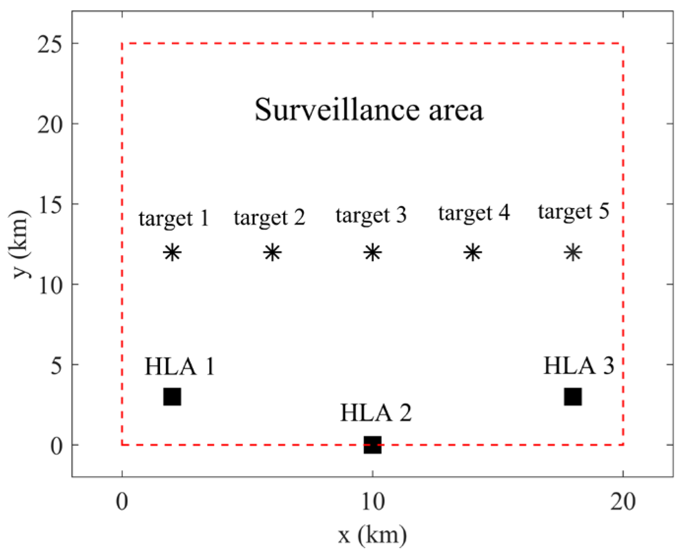
3.2. Localization Performance

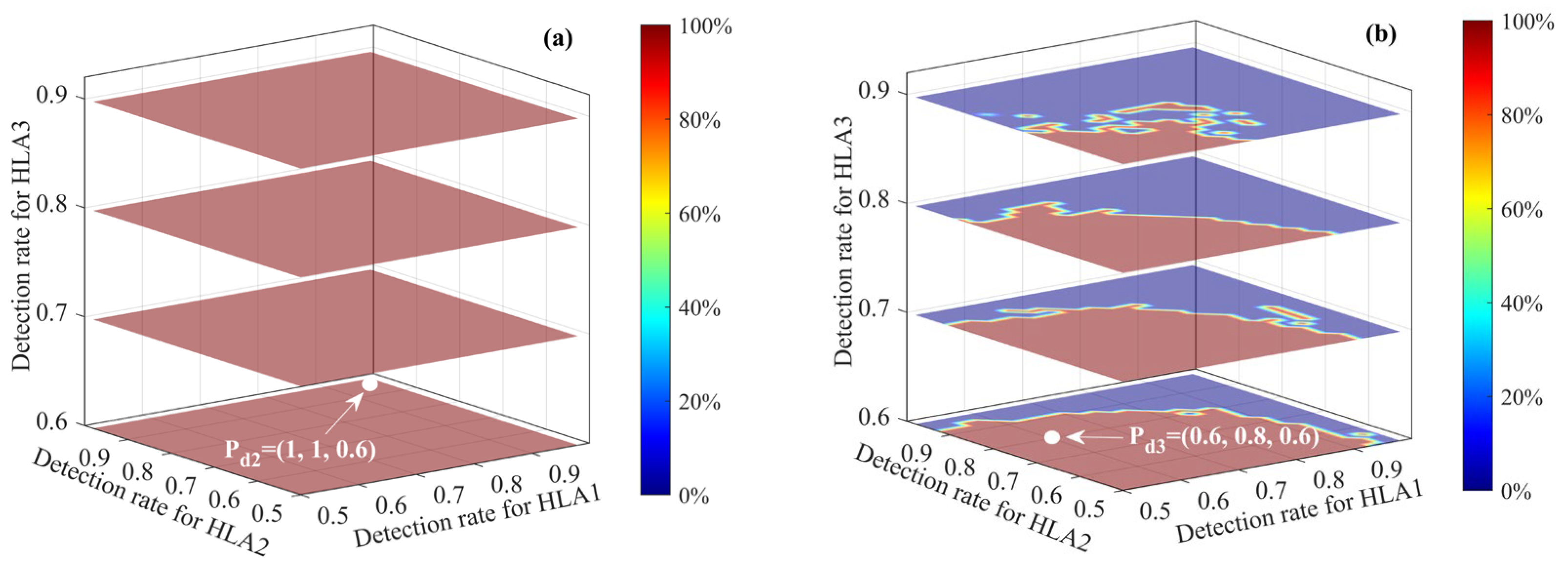
3.2.1. Localization Performance at Different Detection Rates

The surveillance area is a $20 \mathrm{km}\times 25 \mathrm{km}$ rectangular region (see Figure 10). The waveguide environment is identical to that shown in Figure 3. Three identical HLAs, each consisting of 100 equidistantly spaced hydrophones with a length of 198 m, are deployed on the seabed. The reference coordinates are (2 km, 3 km), (10 km, 0 km), and (18 km, 3 km), respectively. The coordinates of the five targets are (2 km, 12 km), (6 km, 12 km), (10 km, 12 km), (14 km, 12 km), and (18 km, 12 km), with a depth of 20 m each. The frequency band of the received signal ranges from 50 Hz to 150 Hz. The averaged received $\overline{\mathrm{SNR}}$ level for each HLA is −5 dB, where $\overline{\mathrm{SNR}}$ is defined as $\overline{\mathrm{SNR}}={\displaystyle \frac{1}{N_d}}{\displaystyle \sum _{n=1}^{N_d}{\mathrm{SNR}}_n}$ and $N_d$ is the number of targets detected by the HLA. The actual detection rates for the HLAs are set as $P_{d1}=(1, 1, 1)$, $P_{d2}=(1, 1, 0.6)$, and $P_{d3}=(0.6, 0.8, 0.6)$, corresponding to the ideal detection rate ($P_{d1}$), the detection rate of one HLA being low ($P_{d2}$) and the detection rates of all HLAs being low ($P_{d3}$). The localization performance for different detection rates is shown in Figure 11a–c. The preset detection rates match the actual detection rates, and the preset measurement error for each HLA is ${\sigma }_s=2^{°}$.

In the ideal measurement scenario with a detection rate of $P_{d1}$, the localization results for all targets can be derived solely from the geometric information of the bearing line intersections. Therefore, both the β-SDA and SDA methods can yield correct localization results (see Figure 11a). As the detection rate decreases, distinguishing between true and ghost targets based on the intersections of bearing lines becomes increasingly difficult. Therefore, the SDA method generates erroneous estimates of both target positions and the number of targets. The β-SDA method correctly estimates the positions of all targets by incorporating waveguide characteristics at detection rates of $P_{d2}$ and $P_{d3}$ (see Figure 11b,c).

For example, consider the analysis of Figure 11c. The localization results from the SDA method are labeled 1 to 4, and those from the β-SDA method are labeled β1 to β5. The localization results 1 and 2 are both derived from the intersections of three bearing lines, resulting in relatively small association costs for them. As a result, the SDA method classifies them as targets after global optimization. The confidence coefficients for the localization results 1 to 4 are 0.62, 0.63, 0.50, and 0.49, respectively. The confidence coefficients for the localization results β1 to β5 are 0.72, 0.84, 0.95, 0.85, and 0.71, respectively. The β-SDA method assigns different confidence coefficients to the intersection points, thereby altering the association costs and enabling the distinction between true and ghost targets.

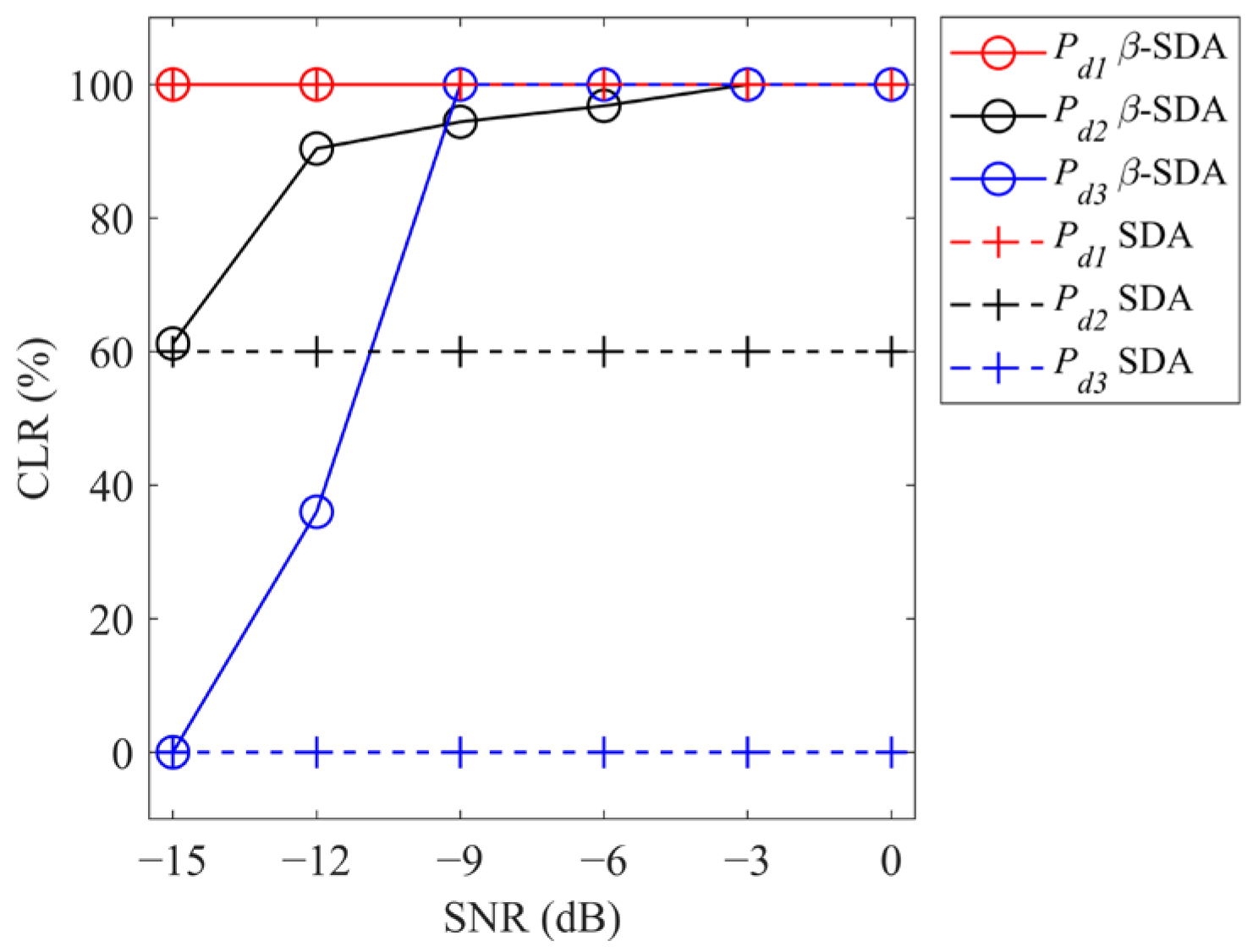
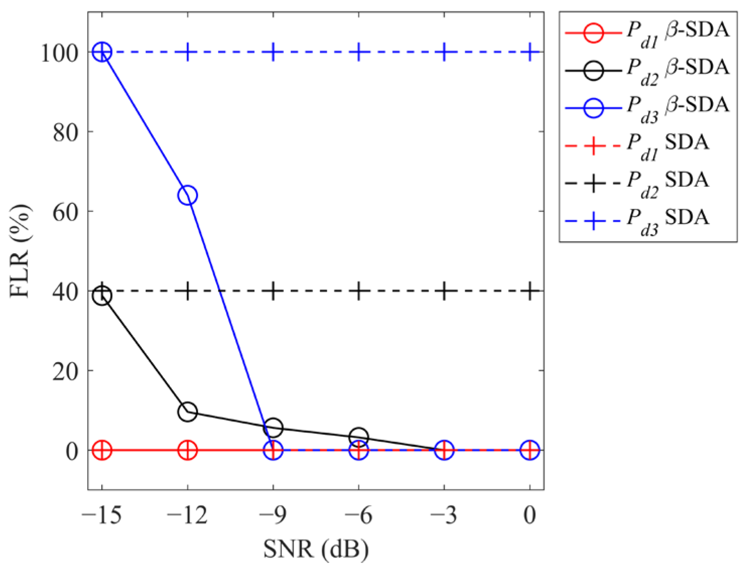
3.2.2. Localization Performance at Different SNR Levels

Noise can degrade the quality of characteristic spectrum, thereby affecting localization performance. The localization performance of the β-SDA and SDA methods is simulated at different averaged received SNR levels, with 100 Monte Carlo trials conducted for each SNR level. The waveguide environment and preset parameters are configured as described in Section 3.2.1. The correct localization rate (CLR) and false localization rate (FLR) of the β-SDA and SDA methods at averaged SNR levels ranging from −15 dB to 0 dB are shown in Figure 12 and Figure 13, respectively. The CLR and FLR are defined as follows:

$$\mathrm{CLR}={\displaystyle \frac{\mathrm{The} \mathrm{number} \mathrm{of} \mathrm{effective} \mathrm{localization} \mathrm{results}}{\mathrm{The} \mathrm{number} \mathrm{of} \mathrm{actual} \mathrm{targets}}},$$

(22)

$$\mathrm{FLR}={\displaystyle \frac{\mathrm{The} \mathrm{number} \mathrm{of} \mathrm{ghost} \mathrm{targets} \mathrm{in} \mathrm{localization} \mathrm{results}}{\mathrm{The} \mathrm{number} \mathrm{of} \mathrm{actual} \mathrm{targets}}},$$

(23)

where the effective localization result ${\widehat{p}}_{eff}$ for an actual target $p_k$ is defined as $\left|{\widehat{p}}_{eff}-p_k\right|\le 800 \mathrm{m}.$

The localization results of the SDA method are determined solely by the geometric information of the output bearing lines. Accurate azimuth results can be obtained for every target at all SNR levels. Therefore, the CLR and FLR of the SDA method remain constant across the received SNR levels. The CLR of the SDA method for detection rates of $P_{d1}$, $P_{d2}$, and $P_{d3}$ are 100%, 60%, and 0%, respectively. The FLR of the SDA method for detection rates of $P_{d1}$, $P_{d2}$, and $P_{d3}$ are 0%, 40%, and 100%, respectively. The β-SDA method significantly improves the accuracy of data association and localization. When the detection rate is $P_{d2}$, the CLR exceeds 90% and the FLR is less than 10% when the averaged SNR level is greater than −12 dB. When the detection rate is $P_{d3}$, the CLR is 100% and the FLR is 0% when the averaged SNR level is greater than −9 dB. The simulation results indicate that the β-SDA method effectively improves the accuracy of the localization results in low detection rate scenarios.

3.2.3. Effect of Preset Parameters on the β-SDA Method

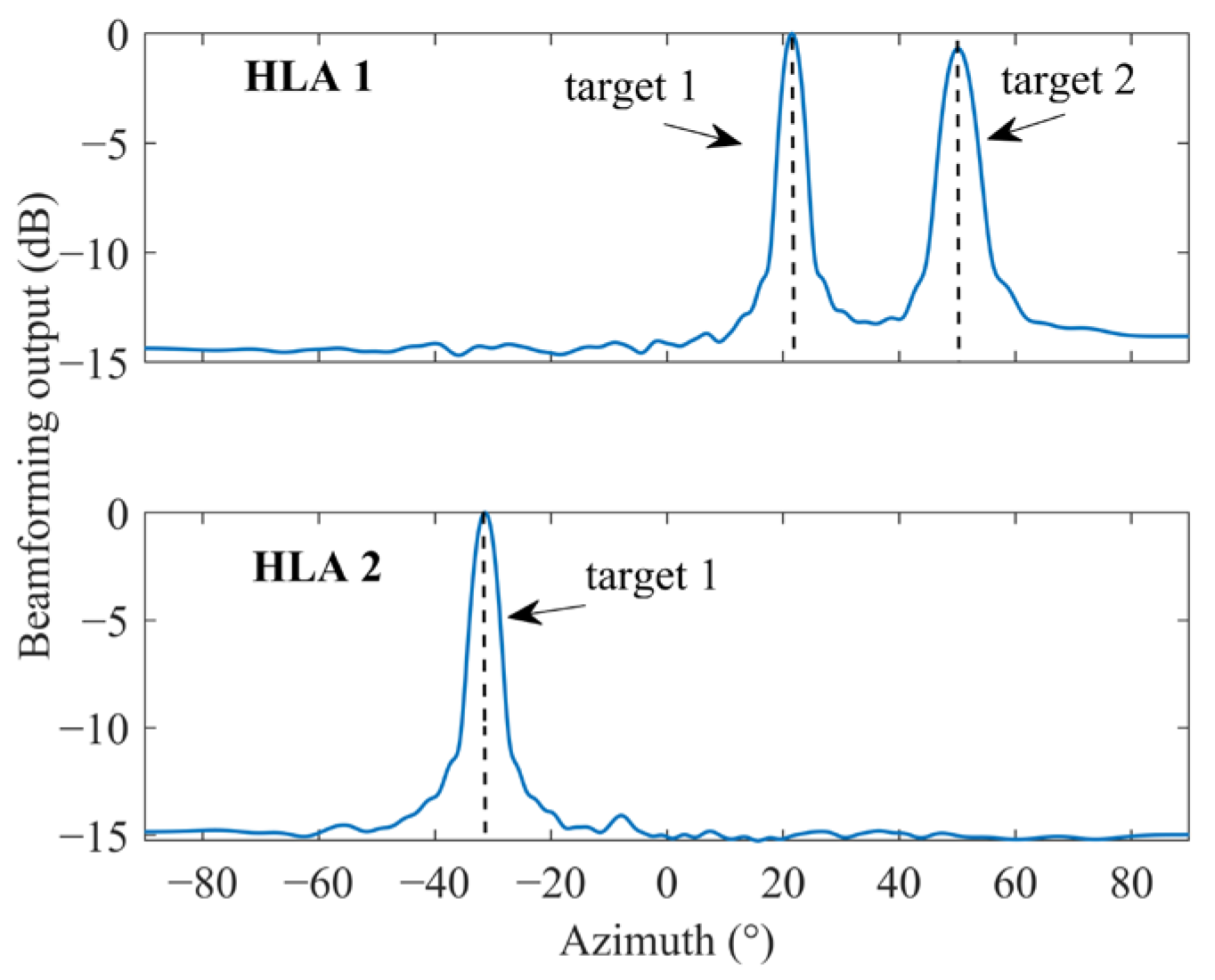
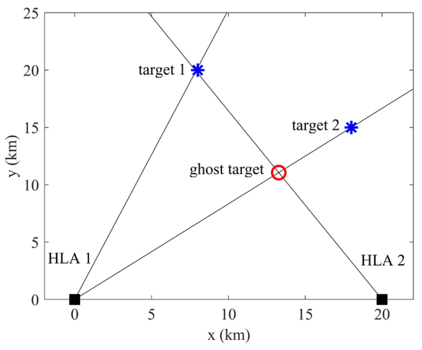
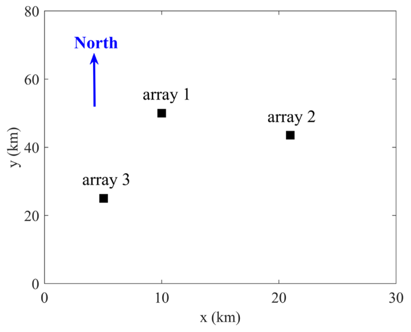
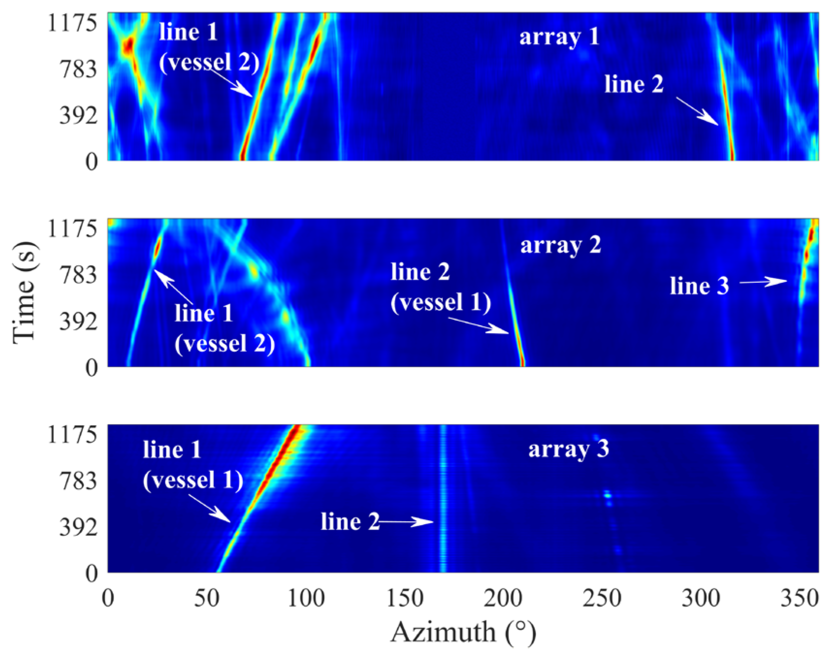
The parameters that must be preset in the method are measurement error $\sigma$ and detection rate $P_d$ of each array. In the underwater acoustic measurement scenarios considered in this article, the targets are typically sparsely distributed in space. Therefore, the method is robust to variations in the selection of measurement errors. Additionally, relatively accurate empirical estimates of measurement errors can be obtained in practice. In the absence of prior information, obtaining an accurate actual detection rate is challenging. Therefore, it is necessary to analyze the effect of the detection rate selection on the β-SDA method’s performance.

The measurement error selected for all HLAs is $\sigma =2^{\circ }$. The actual detection rates are $P_{d2}$ and $P_{d3}$ as defined in Section 3.2.1, and the detection rate range selected for all three HLAs is 0.6 to 0.98. The averaged received SNR is set to −5 dB. The effect of the selected detection rate on the CLR and FLR is shown in Figure 14a,b and Figure 15a,b. The figures show the slices for HLA3 with detection rates selected as 0.6, 0.7, 0.8, and 0.9. The corresponding actual detection rate is labeled in the figure.

When the actual detection rate is $P_{d2}$, corresponding to a lower detection rate of one HLA, targets 3 to 5 are still obtained through the intersections of three bearing lines. The geometric features of the bearing lines are pronounced within the surveillance area. Therefore, correct localization results for all targets can be obtained under different combinations of selected detection rates (see Figure 14a and Figure 15a).

When the actual detection rate is $P_{d3}$, corresponding to low detection rates for all HLAs, correct localization results for all targets can still be obtained as long as the selected detection rate is not significantly greater than the actual detection rate. The association cost for the target corresponding to low detection rates increases sharply when the detection rate selected for a particular array is excessively high (e.g., 0.9 for array 3), leading to a reduction in the tolerance for selecting the detection rate (see Figure 14b and Figure 15b).

The simulation results indicate that the method has some tolerance for the selection of detection rate. The consistency of the CLR and the FLR (see Figure 14 and Figure 15) also indicates that no false targets appear while obtaining the correct localization results for the real target. Based on the conditions of bearing line intersections, the detection rate can be estimated to determine the appropriate input parameter values.

3.3. Sea Trial Data

The trial was conducted in the South China Sea in 2023. The average sea depth of the test area is 96 m, and historical average sound speed data for the same season is used to construct the empirical sound speed profile, as shown in Figure 16. The three arrays are seabed horizontal arrays, consisting of 131, 135, and 140 hydrophones, respectively. The relative position of the arrays is shown in Figure 17.

The sampling rate of the received signal is 5000 Hz, with a total duration of approximately 20 min. The duration of each snapshot is 4.896 s and the frequency range is from 50 Hz to 150 Hz. The β-SDA and SDA methods are used independently to obtain the localization results over the received time period. To mitigate the impact of the source amplitude spectrum and enhance the stability of the β-SDA method, the multi-snapshot azimuth measurement results for each target are used for data association and localization. The measurement error is set to ${\sigma }_s=2^{°}$, and the detection rate for each array is set to 0.8. The bearing-time recording (BTR) obtained through beamforming is shown in Figure 18. The localization performance is shown in Figure 19 where the solid line represents the actual trajectory from the vessel’s AIS, the circular markers represent the localization results of the β-SDA method, and the plus signs represent the localization results of the SDA method.

Each array selects clear and interference-free bearing lines for the measurement. The bearing line 2 output by array 1 does not intersect with the bearing lines output by other arrays, and is therefore excluded from the assignment process based on the constraint conditions (see Figure 18). The β-SDA method yields effective localization results for vessels 1 and 2, while the SDA method results in two false localization outcomes (see Figure 19). The schematic diagram of single-snapshot bearing line intersections is shown in Figure 20. The characteristic spectra corresponding to targets 1 and 2 are shown in Figure 21.

Due to the low detection rate, target 1 (vessel 1) is localized solely by the intersection of bearing lines from arrays 2 and 3, while target 2 (vessel 2) is localized solely by the intersection of bearing lines from arrays 1 and 2. Simultaneously, ghost targets 1 and 2 are present within the surveillance area (see Figure 20). The association costs of targets 1 and 2 for the SDA method are identical to those of ghost targets 1 and 2, making it impossible to correctly locate the actual positions of the vessels. The characteristic spectra of target 1 exhibit a clear frequency structure. Due to interference and noise, the characteristic spectra of target 2 experience clutter interference between 20 Hz and 30 Hz, but still maintain good consistency (see Figure 21). The confidence coefficients for targets 1 and 2 are 0.78 and 0.66, while those for ghost targets 1 and 2 are 0.35 and 0.33, respectively. The association costs for ghost targets 1 and 2 are greater than those for targets 1 and 2 after incorporating waveguide characteristics. Moreover, the constraint condition dictates the number of targets. Therefore, the β-SDA method yields the localization results for all targets within the surveillance area.

The sea trial data processing results indicate that the β-SDA method effectively improves the performance of the assignment algorithm by incorporating waveguide characteristics contained in the beamforming output. In a low detection rate scenario, it offers improved accuracy compared to the traditional bearing line intersection localization method.

4. Conclusions

The β-SDA method for the BOMTL problem is proposed based on the waveguide characteristics contained in the received signals. The estimated distance for each intersection point is obtained from the azimuth measurements, and the characteristic spectrum corresponding to each target is extracted using the warping transformation of the beam output’s autocorrelation function. The bearing lines provide the estimated distance for the warping transformation, while the autocorrelation function avoids the arrival time ambiguity.

Derivations and simulations demonstrated that the frequency corresponding to the peak of the characteristic spectrum is linked to the estimated distance in the warping transformation, while the amplitude of the peak is associated with the depth of the sound source. Based on these characteristics, the β-SDA method was proposed to address the problem of bearing-only multi-target localization using multiple arrays in low detection rate scenarios. The association cost function matrix was optimized using the confidence coefficients derived from waveguide characteristics. The global association results were obtained through the multi-dimensional assignment algorithm, which subsequently obtained the global target position estimation.

Simulations were conducted to assess the localization performance of the β-SDA method under various detection rates, SNR levels, and parameter selections. The results demonstrated that the β-SDA method can overcome the inherent limitation of the pure bearing-only localization. Data association can still be performed even when the geometric features of bearing lines are insufficient to distinguish between real and ghost targets. The correct localization rate is higher and the false localization rate is lower, while the proposed method exhibits a certain tolerance for parameters selection. The sea trial data validated the feasibility of the proposed algorithm. In measurement environments with low detection rates, the β-SDA method effectively localized the positions of the two vessels.

The proposed method requires a certain SNR level, and the effect of the confidence coefficient on the association cost is also influenced by the selection of the preset parameters. Therefore, further research is needed to enhance the reliability of the confidence coefficient in more complex underwater acoustic environments and to select appropriate parameters for different measurement scenarios.

References

1. Cong, L.; Zhuang, W.H. Hybrid TDOA/AOA mobile user location for wideband CDMA-cellular systems. IEEE Trans. Wirel. Commun. 2002, 1, 439–447. [Google Scholar] [CrossRef]
2. Zhang, Y.M.D.; Amin, M.G.; Himed, B. Joint DOD/DOA estimation in MIMO radar exploiting time-frequency signal representations. Eurasip J. Adv. Signal Process. 2012, 2012, 102. [Google Scholar] [CrossRef]
3. Xiong, K.; Cui, G.; Yi, W.; Wang, S.; Kong, L. Distributed localization of target for MIMO radar with widely separated directional transmitters and omnidirectional receivers. IEEE Trans. Aerosp. Electron. Syst. 2022, 59, 3171–3187. [Google Scholar] [CrossRef]
4. Kim, J. Locating an Underwater Target Using Angle-Only Measurements of Heterogeneous Sonobuoys Sensors with Low Accuracy. Sensors 2022, 22, 3914. [Google Scholar] [CrossRef] [PubMed]
5. Wang, L.; Yang, Y.; Liu, X. A distributed subband valley fusion (DSVF) method for low frequency broadband target localization. Acoust. Soc. Am. J. 2018, 143, 2269–2278. [Google Scholar] [CrossRef]
6. Deb, S.; Pattipati, K.R.; Bar-Shalom, Y.; Washburn, R.B. Assignment Algorithms for the Passive Sensor Data Association Problem. Proc. SPIE Int. Soc. Opt. Eng. 1989, 1096, 231–243. [Google Scholar]
7. Bar-Shalom, Y.; Willett, P.K.; Tian, X. Tracking and Data Fusion; YBS Publishing: Storrs, CT, USA, 2011; Volume 11. [Google Scholar]
8. Su, Z.; Ji, H.; Zhang, Y. Loopy belief propagation based data association for extended target tracking. Chin. J. Aeronaut. 2020, 33, 2212–2223. [Google Scholar] [CrossRef]
9. Gavish, M.; Weiss, A.J. Performance analysis of bearing-only target location algorithms. IEEE Trans. Aerosp. Electron. Syst. 1992, 28, 817–828. [Google Scholar] [CrossRef]
10. Dogançay, K. Bearings-only target localization using total least squares. Signal Process. 2005, 85, 1695–1710. [Google Scholar] [CrossRef]
11. Abatzoglou, T.J.; Mendel, J.M. The constrained total least squares technique and its applications to harmonic superresolution. Signal Process. IEEE Trans. 1991, 39, 1070–1087. [Google Scholar] [CrossRef]
12. Bishop, A.N.; Pathirana, P.N. Localization of emitters via the intersection of bearing lines: A ghost elimination approach. IEEE Trans. Veh. Technol. 2007, 56, 3106–3110. [Google Scholar] [CrossRef]
13. Oshman, Y.; Davidson, P. Optimization of observer trajectories for bearings-only target localization. IEEE Trans. Aerosp. Electron. Syst. 1999, 35, 892–902. [Google Scholar] [CrossRef]
14. Bar-Shalom, Y.; Jaffer, A.G. Adaptive nonlinear filtering for tracking with measurements of uncertain origin. In Proceedings of the 1972 IEEE Conference on Decision and Control and 11th Symposium on Adaptive Processes, New Orleans, NY, USA, 13–15 December 1972; pp. 243–247. [Google Scholar]
15. Reed, J.D.; da Silva, C.R.; Buehrer, R.M. Multiple-source localization using line-of-bearing measurements: Approaches to the data association problem. In Proceedings of the MILCOM 2008–2008 IEEE Military Communications Conference, San Diego, CA, USA, 16–19 November 2008; pp. 1–7. [Google Scholar]
16. Gardner, W.; Brown, W.; Chih-Kang, C. Spectral Correlation of Modulated Signals: Part II—Digital Modulation. IEEE Trans. Commun. 1987, 35, 595–601. [Google Scholar] [CrossRef]
17. Xu, L.; Yang, Y. Parameter estimation of underwater moving sources by using matched Wigner transform. Appl. Acoust. 2016, 101, 5–14. [Google Scholar] [CrossRef]
18. Avitzour, D. A maximum likelihood approach to data association. IEEE Trans. Aerosp. Electron. Syst. 1992, 28, 560–566. [Google Scholar] [CrossRef]
19. Poore, A.P.; Rijavec, N. A Lagrangian relaxation algorithm for multidimensional assignment problems arising from multitarget tracking. SIAM J. Optim. 1993, 3, 544–563. [Google Scholar] [CrossRef]
20. Deb, S.; Yeddanapudi, M.; Pattipati, K.; BarShalom, Y. A generalized S-D assignment algorithm for multisensor-multitarget state estimation. IEEE Trans. Aerosp. Electron. Syst. 1997, 33, 523–538. [Google Scholar] [CrossRef]
21. Popp, R.L.; Pattipati, K.R.; Bar-Shalom, Y. m-best S-D assignment algorithm with application to multitarget tracking. Aerosp. Electron. Syst. IEEE Trans. 1998, 37, 22–39. [Google Scholar] [CrossRef]
22. Bonnel, J.; Nicolas, B.; Mars, J.I.; Walker, S.C. Estimation of modal group velocities with a single receiver for geoacoustic inversion in shallow water. J. Acoust. Soc. Am. 2010, 128, 719–727. [Google Scholar] [CrossRef] [PubMed]
23. Yu-Bo, Q.; Shi-Hong, Z.; Ren-He, Z.; Yun, R. A passive source ranging method using the waveguide-invariant-warping operator. Acta Phys. Sin. 2015, 64, 074301. [Google Scholar] [CrossRef]
24. Yang, T.C. Beam intensity striations and applications. J. Acoust. Soc. Am. 2003, 113, 1342–1352. [Google Scholar] [CrossRef] [PubMed]
25. Arnol’d, V.I. Remarks on the stationary phase method and Coxeter numbers. Russ. Math. Surv. 1973, 28, 19–48. [Google Scholar] [CrossRef]
26. Nardone, S.C.; Aidala, V.J. Observability criteria for bearings-only target motion analysis. IEEE Trans. Aerosp. Electron. Syst. 1981, AES-17, 162–166. [Google Scholar] [CrossRef]
27. Porter, M.B.; Reiss, E.L. A numerical method for bottom interacting ocean acoustic normal modes. J. Acoust. Soc. Am. 1985, 77, 1760–1767. [Google Scholar] [CrossRef]
28. Bonnel, J.; Chapman, N.R. Geoacoustic inversion in a dispersive waveguide using warping operators. J. Acoust. Soc. Am. 2011, 130, EL101–EL107. [Google Scholar] [CrossRef]
29. Yang, X.; Li, F.; Zhang, B.; Luo, W. Seasonally-invariant head wave speed extracted from ocean noise cross-correlation. J. Acoust. Soc. Am. 2020, 147, EL241–EL245. [Google Scholar] [CrossRef] [PubMed]
30. Wen-Hua, S.; Ning, W.; Da-Zhi, G.; Hao-Zhong, W.; Ke, Q. Concept of waveguide invariant spectrum and algorithm for its extraction. Acta Phys. Sin. 2017, 66, 114301. [Google Scholar] [CrossRef]
31. Niu, H.; Zhang, R.; Li, Z. Theoretical analysis of warping operators for non-ideal shallow water waveguides. J. Acoust. Soc. Am. 2014, 136, 53–65. [Google Scholar] [CrossRef]
Figure 1. Schematic diagram of the two-dimensional bearing-only multi-target localization model.
Jmse 12 02300 g001
Figure 2. Block diagram of the β-SDA method.
Jmse 12 02300 g002
Figure 3. Sound speed profile.
Jmse 12 02300 g003
Figure 4. Beamforming outputs of HLA 1 and HLA 2.
Jmse 12 02300 g004
Figure 5. Intersections of the bearing lines.
Jmse 12 02300 g005
Figure 6. Characteristic spectra of target 1.
Jmse 12 02300 g006
Figure 7. Comparison of the correlation coefficients for target 1 and ghost target, with the average received SNR ranging from −15 dB to 0 dB.
Jmse 12 02300 g007
Figure 8. Normalized amplitude of the characteristic spectrum for target 1 output by HLA 1. Source frequency bands: (a) 50–150 Hz. (b) 100–200 Hz.
Jmse 12 02300 g008
Figure 9. Correlation coefficient for target 1 and ghost target. Source frequency bands: (a) 50–150 Hz. (b) 100–200 Hz.
Jmse 12 02300 g009
Figure 10. Positions of the HLAs and targets.
Jmse 12 02300 g010
Figure 11. Localization performance at different detection rates. (a) P d 1 = ( 1 ,   1 ,   1 ) . (b) P d 2 = ( 1 ,   1 ,   0 . 6 ) . (c) P d 3 = ( 0.6 ,   0.8 ,   0.6 ) .
Jmse 12 02300 g011
Figure 12. Correct localization rate.
Jmse 12 02300 g012
Figure 13. False localization rate.
Jmse 12 02300 g013
Figure 14. Variation in the CLR with respect to the selected detection rate. (a) Actual detection rate is P d 2 = ( 1 ,   1 ,   0 . 6 ) . (b) Actual detection rate is P d 3 = ( 0.6 ,   0.8 ,   0.6 ) .
Jmse 12 02300 g014
Figure 15. Variation in the FLR with respect to the selected detection rate. (a) Actual detection rate is P d 2 = ( 1 ,   1 ,   0 . 6 ) . (b) Actual detection rate is P d 3 = ( 0.6 ,   0.8 ,   0.6 ) .
Jmse 12 02300 g015
Figure 16. Empirical sound speed profile.
Jmse 12 02300 g016
Figure 17. The relative position of the arrays.
Jmse 12 02300 g017
Figure 18. BTR of the three arrays.
Jmse 12 02300 g018
Figure 19. Localization performance.
Jmse 12 02300 g019
Figure 20. Intersections of the bearing lines.
Jmse 12 02300 g020
Figure 21. Characteristic spectra corresponding to targets 1 and 2.
Jmse 12 02300 g021