Research on the Differential Model-Free Adaptive Mooring Control Method for Uncrewed Wave Gliders

Abstract

Uncrewed Wave Gliders (UWGs) are capable of harnessing energy from ocean waves and photovoltaic sources to enable long-duration voyages. Since the float’s yaw motion relies on the rudder of the submersible for control, this introduces many unknown nonlinear and time-delay factors into the control system. Moreover, the susceptibility of UWGs to waves influences results in limited maneuverability and necessitates energy efficiency considerations, complicating the task of following a designated path to a specific point for observations. To address these challenges, this paper first introduces a differential model-free adaptive control (DMFAC) approach for managing the float’s heading control, along with a proof of its stability. Furthermore, an improved attractive force line-of-sight (IAFLOS) guidance strategy for overall mooring control is proposed. The integration of the DMFAC heading controller and the IAFLOS strategy forms a comprehensive mooring control system, which is validated through simulation studies in typical maritime conditions. This control system ensures that, while considering energy conservation strategies, the distance between the wave glider and the mooring point remains within 20 m during mooring.

1. Introduction

The Uncrewed Wave Glider (UWG) is a novel type of oceanic vessel that captures energy from ocean waves and mechanically converts it into propulsion [1,2,3]. Solar panels are employed to absorb solar energy, providing power for the UWG control system. This innovative mode of operation theoretically offers the wave glider infinite power, zero pollution, and low-consumption benefits [4,5,6]. Due to these characteristics, wave gliders are extensively used in a wide range of scientific research tasks, including meteorological observation and marine hydrological environment surveys [7,8,9]. The UWG consists of a float, a submersible, and a flexible tether cable that connects the float and the submersible [10]. The float is equipped with various sensors, GPS, and solar panels, while the submersible carries servomechanisms, a magnetic compass, and some hydrofoils. As the float rises, the submersible ascends along with it due to the tension in the tether cable; when the float descends, the submersible, having a greater overall density than water, also moves downward under the force of gravity, as illustrated in Figure 1. Due to the decrease in wave amplitude with increasing water depth, the water around the submersible does not move like the surface waves [11,12,13]. The UWG’s principle of movement is shown in Figure 1.

For the Uncrewed Wave Glider (UWG), many oceanic water quality long-duration observations involve reaching a target point via a predetermined path and then conducting stationary observations at mooring [14]. In horizontal motion, as only the submersible part is equipped with a rudder, the float’s heading movement depends solely on the towing action of the submersible part, resulting in significant inertia and time delay in the control system. Therefore, the direct application of traditional heading control methods, such as PID and sliding mode control, often leads to oscillations and divergence [15,16,17]; whereas model-driven control algorithms like sliding mode and backstepping require a precise mathematical model of the UWG [18,19,20]. However, the complex and highly coupled structure of the UWG makes it difficult to establish an accurate mathematical model, which can lead to unstable or even uncontrollable conditions. A floating body heading control method based on the multi-body dynamic model of wave gliders was proposed [21], but its high requirements for model precision limit its practical engineering application. A floating body heading control method based on a sliding time window was also proposed [22], but this method suffers from slow convergence due to the time window period limitation. Inspired by the idea of a model-independent redefined model-free adaptive heading control method [23], a differential model-free adaptive control (DMFAC) method for the UWG float’s heading control system, a strongly nonlinear coupled system, is proposed. Through constructing a criterion function that satisfies the Lipschitz condition independent of the specific UWG mathematical model, a robust control law for nonlinear systems has been established.

For the UWG, which is heavily influenced by waves and has limited maneuverability, the ocean current speed can be comparable to its own speed. Therefore, while following a predetermined path to a mooring target point, significant displacement can occur under strong currents. Once the impact of the currents diminishes, the UWG may find itself too far from the intended path, and traditional line-of-sight (LOS) guidance laws might be insufficient to return the UWG to its desired route [24,25,26]. The integral process included in LOS guidance laws could prevent the UWG from converging back to the desired path in a timely manner due to persistent current effects, resulting in excessive error integration that undermines control effectiveness. To address these challenges, this paper proposes an improved attractive force line-of-sight (IAFLOS) guidance strategy. In this strategy, multiple attractive forces are designed at several critical positions along the desired path to ensure that the UWG can accurately follow and return to near the target path points, even with significant deviations, thus minimizing overshoot and continuing the path-following task. Once the UWG reaches the mooring point, the attractive force is simplified and set only at the mooring point to ensure that the UWG can perform mooring control tasks near the mooring point while considering energy conservation.

In summary, the main contributions of this paper are as follows:

• Differential Model-Free Adaptive Control Method for Float Heading: Addressing the strong nonlinear coupling and time-delay issues in the heading control of UWG floats, we propose a differential model-free adaptive control method. Establishing a new criterion function makes the heading control subsystem match the dynamic speed change in MFAC and demonstrates good disturbance resistance.
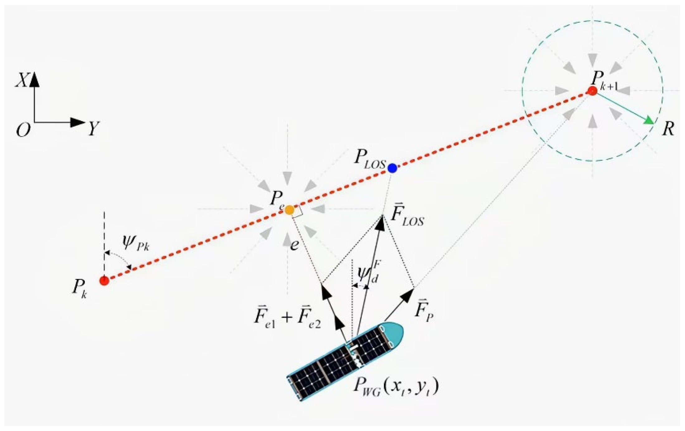
• Improved Gravitational Vector LOS Guidance Strategy for UWGs: For UWGs with limited maneuverability and significant susceptibility to ocean currents, we developed an improved gravitational vector LOS guidance strategy. This strategy involves setting different gravitational terms along the path and updating the integral terms under various conditions. This ensures that the UWG can stably follow the designated path and reach the mooring point. During the mooring process, gravitational forces are only present at the mooring point with energy conservation in mind, and conditions for the presence of gravitational forces are set to ensure the smooth completion of mooring control while achieving energy savings.

2. Mathematical Modeling and Theoretical Foundations

2.1. Mathematical Modeling

For the special structure of wave gliders, three body-fixed coordinate systems and one fixed terrestrial coordinate system are defined to describe their mathematical models. The origins of the body-fixed coordinate systems are, respectively, located at the center of gravity of the float, the center of gravity of the Submersible, and the overall center of gravity of the wave glider system [27]. The established coordinate system is shown in Figure 2:

The axes $x^F,x^G$ are selected to point toward the bow directions of the float and the submersible, respectively, with an axis pointing in the forward direction of the UWG, and axis $z^0$ directed downward along the tether. The mathematical model for the UWG’s motion is established by selecting six independent degrees of freedom: the longitudinal and lateral motions of the UWG system’s center of gravity, the roll and pitch motions of the tether, and the yaw motions of both the float and the submersible. The mathematical model is formulated as follows [28,29]:

$${\mathbf{M}}_{RB} \dot{\mathbf{v}}+{\mathbf{F}}_{MA}({\mathbf{v}}_r)+{\mathbf{C}}_{RB}(\mathbf{v})\mathbf{v}+{\mathbf{F}}_{CA}({\mathbf{v}}_r)+\mathbf{D}({\mathbf{v}}_r)+\mathbf{g}(\mathbf{\eta })=\mathbf{\tau }$$

(1)

In the model, ${\mathbf{M}}_{RB}$ represents a rigid body mass matrix, ${\mathbf{F}}_{MA}({\mathbf{v}}_r)$ denotes a hydrodynamic inertia vector, ${\mathbf{C}}_{RB}$ is a matrix of Coriolis–centripetal coefficients, ${\mathbf{F}}_{CA}({\mathbf{v}}_r)$ is a Coriolis-like force vector, $\mathbf{D}({\mathbf{v}}_r)$ is a damping force vector, $\mathbf{g}(\mathbf{\eta })$ stands for a restoring force vector, $\mathbf{\tau }$ indicates an active control force vector, and $\mathbf{v}$ is a velocity vector for the six degrees of freedom.

Under the rise and fall of waves, the buoyant float of the wave glider moves up and down with the waves. When the float rises, the tethered glider is pulled upward by the tension in the cable. When the float descends, the glider sinks due to its overall density being greater than that of water, as well as the effect of gravity. Since the amplitude of the waves decreases with depth, the surrounding water near the glider does not move in the same way as the surface waves. This creates relative motion between the glider and the surrounding water in the vertical direction. The water wings on the glider are connected to the body through the $z^0$, with the axis positioned near the leading edge of the wing. The trailing edge of the wing is free to rotate around the axis. During the upward motion of the glider, the trailing edge of the water wing swings downward under the influence of the water flow. This generates lift on the water wing, directed toward the $x^G$. When the glider descends, the wing’s orientation is reversed, and the trailing edge swings upward. The direction of the water flow also reverses, and lift is once again generated on the water wing, directed toward the $x^G$. Thus, regardless of the direction of the waves, as long as the wave glider rises and falls with the waves, the glider will convert the vertical motion energy into forward thrust through its unique mechanical structure, propelling it forward by towing the float via the cable. This propulsion method offers significant advantages such as zero emissions and low noise. Moreover, compared to traditional marine vehicles, the entire process relies solely on the continuous wave energy from the ocean, with no need for additional energy input. This enables the wave glider to have virtually unlimited endurance.

2.2. MFAC Theory

A Single-Input Single-Output (SISO) nonlinear system operating offline can be described as follows [30,31,32,33]:

$$y(k+1)=f(y(k),\dots ,y(k-n_y),u(k),\dots ,u(k-n_u))$$

(2)

where $u(k)$ represents the system’s input, $y(t)$ denotes the system’s output, and $t$ represents the time instant.

We make the assumptions for the system (2):

Assumption 1. 

The partial derivatives of $f(\cdot )$ exist and are continuous.

Assumption 2. 

Except for a finite number of instants, $f(\cdot )$ satisfies the generalized Lipschitz condition, which states that at any time $t$ and for all $i_1$ and $i_2$, $u(i_1)\ne u\left(i_2\right)$, it holds that

$$\left|y(i_1+1)-y(i_2+1)\right|\le L\left|u(i_1)-u(i_2)\right|$$

(3)

 where $L$is a constant.

Assumption 1 is a fundamental assumption for the design of control systems. Assumption 2 limits the upper bound on the rate of change in the system’s output, a condition commonly encountered in many motion control systems and physical processes.

Lemma 1. 

For a system that satisfies Assumptions 1 and Assumption 2, when $\left|∆u(k)\ne 0\right|$, there must be a time-varying coefficient $\varphi (k)\in ℝ$ such that system (2) can be transformed into the following mathematical model:

$$∆y(k+1)=\varphi (k)∆u(k)$$

(4)

where $\varphi (k)$ is the PDD parameter [34], and it is bounded at any given moment.

Therefore, this model can also be represented as

$$y(k+1)-y(k)=\varphi (k)(u(k)-u(k-1))$$

(5)

In controller design, nonlinear systems can be linearized using the PDD method. PDD serves as a time-varying parameter of the model, encapsulating the time-varying and nonlinear characteristics of the controlled system. For simple nonlinear systems, PDD represents the derivative of the nonlinear system with respect to the control input at the current moment.

Lemma 2. 

$a+b\ge 2\sqrt{ab}$, where $a\ge 0,b\ge 0$

3. Design of Mooring Control Scheme for UWG

3.1. Design of Heading Controller for Wave Glider Float

From the analysis, it is known that the heading response of the float is due to the heading difference between the float and the submersible, and the tether generates a turning moment at the connection point on the float relative to its center of gravity. Therefore, if the wave glider’s float is to reach a desired heading, the submersible should be steered to a specific desired submersible heading by controlling its rudder, thus generating the desired turning moment on the float to turn its heading to the desired position. Since the float cannot respond immediately when a heading difference occurs, the control process of the float involves a time delay.

If the rudder angle generated by Submersible’s rudder response is denoted as $\delta$, then the float heading control system can be defined as follows:

$$\left\{\begin{array}{l}{\dot{\psi }}^F=r^F\\ {\dot{r}}^F=\delta (t-\epsilon )+\vartheta \end{array}\right.$$

(6)

where ${\psi }^F$ represents the current heading of the float, $\vartheta$ accounts for disturbances from unmodeled parts of the system and environmental effects, and $\delta$ symbolizes the effective lagged rudder angle. And the equivalent rudder angle of the floating body is mathematically defined as the difference between the heading of the sub and the heading of the float at the current moment: $\delta ={\psi }^G-{\psi }^F$, where ${\psi }^G$ represents the current heading of the glider. $\delta (t-\epsilon )$ represents the equivalent rudder angle of the delayed float, which can be described as the combination of an immediate rudder angle response and an additional lag compensation term for the rudder angle.

$$\delta (t-\epsilon )=\delta +\mathrm{\Xi }(\delta ,\epsilon )$$

(7)

Since the heading range of the Unmanned Wave Glider (UWG) varies in the range [−180°, 180°], it fails to satisfy the Lipschitz condition. Additionally, in the heading system, the output of the control system is the rudder angle rather than the directly controlled heading, which leads to a conflict between the dynamic change rate of the control subsystem and the MFAC. Therefore, a DMFAC method was designed to manage the heading control of the wave glider’s float.

A criterion function was designed as follows:

$$\begin{array}{ll}J(\delta (k))& =({\psi }^{\ast }(k+1)-\psi (k){)}^2+\lambda (\delta (k)-\delta (k-1){)}^2\\ & +2k_r{\displaystyle \frac{∆\psi (k+1)\psi (k)}{T_s}}\end{array}$$

(8)

where $T_s$ represents the sampling time of the control system, $k_r$ is the introduced weighting coefficient, and ${\psi }^{\ast }(k+1)$ represents the expected output of the system.

To derive the control law, differentiate Equation (8) with respect to $\delta (k)$, normalize certain constant parameters, and set the equation equal to zero to obtain the following control law:

$$\begin{array}{ll}\delta (k)& =\delta (k-1)+{\displaystyle \frac{\widehat{\varphi }(k)}{\lambda +{\left|\widehat{\varphi }(k)\right|}^2}}(\psi (k+1{)}^{\ast }-\psi (k))-k_r{\displaystyle \frac{\widehat{\varphi }(k)∆\psi (k)}{\lambda +{\left|\widehat{\varphi }(k)\right|}^2}}\\ & =\delta (k-1)+{\displaystyle \frac{\eta \widehat{\varphi }(k)}{\lambda +{\left|\widehat{\varphi }(k)\right|}^2}}(\psi (k+1{)}^{\ast }-\psi (k)-k_r{\displaystyle \frac{\widehat{\varphi }(k)∆\psi (k)}{{{\rm T}}_s(\lambda +{\left|\widehat{\varphi }(k)\right|}^2)}})\end{array}$$

(9)

In this control law, $\eta \in (0,1)$ represents the step size factor, and $\lambda >0$ is the weighting coefficient.

The PPD estimation algorithm is designed based on the I/O data of the controlled system. We propose the following criterion function for PDD:

$$J(\varphi (k))={\left|\psi (k)-\psi (k-1)-\varphi (k)∆\delta (k-1)\right|}^2+\varpi {\left|\varphi (k)-{\widehat{\varphi }}_c(k)\right|}^2$$

(10)

where $\varpi$ is the weighting coefficient, and $\widehat{\varphi }(k)$ is the estimated value of $\varphi (k)$.

To find the extremum of Equation (10) with respect to the PDD $\varphi (k)$, we obtain

$$\widehat{\varphi }(k)=\widehat{\varphi }(k-1)+{\displaystyle \frac{\kappa ∆\delta (k-1)}{\mu +∆\delta {(k-1)}^2}}(∆\psi (k)-\widehat{\varphi }(k-1))∆\delta (k-1)$$

(11)

And $\widehat{\varphi }(k)=\widehat{\varphi }(1)$ when $\left|\widehat{\varphi }(k)\right|\le \iota$, $\left|∆\delta (k-1)\right|\le \iota$ or $\mathrm{sign}(\widehat{\varphi }(k))\ne \mathrm{sign}(\widehat{\varphi }(1))$.

3.2. Design of IAFLOS Mooring Control Scheme

In response to the significant drift and potential loss of control experienced by traditional LOS wave gliders under the influence of ocean currents, this paper proposes an IAFLOS mooring control scheme strategy. The overall strategy and guidance diagram is shown in Figure 3:

The overall mooring process can be divided into two phases: the path-following stage before reaching the mooring point and the mooring stage after reaching it. Let the mooring point be $P_f$, and the desired path point before reaching the mooring be $P_k,P_{k+1}$. From the current position $P_{WG}(x_t,y_t)$ of the UWG, a perpendicular line is drawn to the desired path, with the perpendicular foot at $P_k{P}_{k+1}$. The target path point $P_{k+1}$ and the point $P_e$ each have gravitational fields; the gravitational field at $P_{k+1}$ is constant and unchanging. Due to the movement of the UWG, point $P_e$ continuously changes, and therefore, the gravitational field at point $P_e$ moves as $P_e$ changes. The gravitational force felt by the wave glider at its current position $P_{WG}$ from point $P_{k+1}$ is ${\stackrel{\rightharpoonup }{F}}_p$, which guides the wave glider toward the target point $P_{k+1}$. The direction and calculation method of ${\stackrel{\rightharpoonup }{F}}_p$ are as follows:

$${\stackrel{\rightharpoonup }{F}}_p={\xi }_1{\displaystyle \frac{\stackrel{\rightharpoonup }{P_{WG}{P}_{k+1}}}{‖P_{WG}{P}_{k+1}‖}}$$

(12)

where ${\xi }_1$ is a design parameter, with the direction being from the wave glider toward path point $P_{k+1}$.

There are two different attractive forces at the point $P_e$, denoted as ${\stackrel{\rightharpoonup }{F}}_{e1}$ and ${\stackrel{\rightharpoonup }{F}}_{e2}$, which ${\stackrel{\rightharpoonup }{F}}_{e1}$ is set as follows:

$$\stackrel{\rightharpoonup }{F_{e1}}={\xi }_2\stackrel{\rightharpoonup }{P_{WG}{P}_e}$$

(13)

where ${\xi }_2$ is a design parameter. When the wave glider is on the desired path, $\stackrel{\rightharpoonup }{F_{e1}}$ is 0. When the wave glider deviates from the desired path, the magnitude of $\stackrel{\rightharpoonup }{F_{e1}}$ increases, as the absolute value of the lateral tracking error of the wave glider increases, and its direction always points from the wave glider’s current position toward point $P_e$.

If the resultant direction of gravitational forces ${\stackrel{\rightharpoonup }{F}}_p$ and ${\stackrel{\rightharpoonup }{F}}_{e1}$ is used solely as the desired heading for the wave glider, under the influence of ocean currents, it is possible that the wave glider’s velocity component in the direction of ${\stackrel{\rightharpoonup }{F}}_{e1}$ may become equal in magnitude but opposite in direction to the current velocity. In this case, the wave glider will no longer move closer to the desired path, and the resultant direction of the gravitational forces ${\stackrel{\rightharpoonup }{F}}_p$ and ${\stackrel{\rightharpoonup }{F}}_{e1}$ will no longer change, resulting in a steady-state error, which affects the path-following control accuracy. Therefore, an additional gravitational force is introduced at point $P_e$:

$${\stackrel{\rightharpoonup }{F}}_{e2}={\xi }_3{\displaystyle \sum _{i=0}^t\stackrel{\rightharpoonup }{P_{WG}{P}_e}}{|}_i$$

(14)

where ${\xi }_3$ is a design parameter. When calculating according to Equation (14), if the UWG stays close to the desired path for an extended period, ${\stackrel{\rightharpoonup }{F}}_{e2}$ will accumulate and become large, causing the UWG to overshoot the desired path, resulting in significant overshoot and increasing the adjustment time of the control system. To address this issue, the calculation of ${\stackrel{\rightharpoonup }{F}}_{e2}$ was improved, and the following update law was designed:

$$\left\{\begin{array}{l}\begin{array}{ccc}{\stackrel{\rightharpoonup }{F}}_{e2}(t+1)={\stackrel{\rightharpoonup }{F}}_{e2}(t)+\chi {\xi }_3\stackrel{\rightharpoonup }{P_{WG}{P}_e}(t)& & {\stackrel{\rightharpoonup }{F}}_{e2}(t)\stackrel{\rightharpoonup }{P_{WG}{P}_e}(t)<0\end{array}\\ \begin{array}{ccc}{\stackrel{\rightharpoonup }{F}}_{e2}(t+1)={\stackrel{\rightharpoonup }{F}}_{e2}(t)+{\xi }_3\stackrel{\rightharpoonup }{P_{WG}{P}_e}(t)& & {\stackrel{\rightharpoonup }{F}}_{e2}(t)\stackrel{\rightharpoonup }{P_{WG}{P}_e}(t)\ge 0\end{array}\end{array}\right.$$

(15)

where $\chi >0$ represents the amplification factor.

The total gravitational force acting on the floating body at present is thus obtained:

$${\stackrel{\rightharpoonup }{F}}_{LOS}={\stackrel{\rightharpoonup }{F}}_P+{\stackrel{\rightharpoonup }{F}}_{e_1}+{\stackrel{\rightharpoonup }{F}}_{e2}$$

(16)

To prevent the absolute value of the lateral tracking error $\left|e\right|$ from becoming too large, which could also cause cumulative ${\stackrel{\rightharpoonup }{F}}_{e2}$ to increase significantly and cause the UWG trajectory to oscillate repeatedly, a maximum deviation threshold $e_{\max }$ is introduced. Based on whether $e_{\max }$ is exceeded by $\left|e\right|$, the current UWG desired heading angle calculation strategy is set:

(1) If $\left|e\right|<e_{\max }$, set the current desired heading of the floating body to the ${\stackrel{\rightharpoonup }{F}}_{LOS}$ direction;

(2) If $\left|e\right|>e_{\max }$, set the desired heading of the floating body to the ${\stackrel{\rightharpoonup }{F}}_{e_1}$ direction and reset ${\stackrel{\rightharpoonup }{F}}_{e2}$ to zero until $\left|e\right|<e_{\max }$. In other words,

$$\left\{\begin{array}{l}{\psi }_d^F=\mathrm{atan}2(x_{pe}-x_t,y_{pe}-y_t)\\ {\stackrel{\rightharpoonup }{F}}_{e2}=(0,0)\end{array}\right.$$

(17)

When the UWG reaches mooring point $P_f$, at this time, only the gravitational force ${\stackrel{\rightharpoonup }{F}}_P$ from $P_f$ exists in the gravitational field, while all other gravitational forces ${\stackrel{\rightharpoonup }{F}}_{e1},{\stackrel{\rightharpoonup }{F}}_{e2}$ are set to zero. To conserve energy, a radius of influence $R_f$ is defined. If the distance from the UWG to the mooring point exceeds $R_f$, the gravitational force is reintroduced for calculation.

The entire mooring strategy is outlined in Algorithm 1.

Algorithm 1: IAFLOS Mooring Guidance Strategy

Given: $\mathrm{Target} \mathrm{path} \mathrm{point} P_1(x_1,y_1),P_2(x_2,y_2)\dots \dots P_n(x_n,y_n)$, $\mathrm{Mooring} \mathrm{point} P_n$,

$\hspace{1em}\hspace{1em}\hspace{1em}\hspace{1em}\hspace{1em}\hspace{1em}\hspace{1em}\hspace{1em}\hspace{1em}\hspace{1em}\hspace{1em}\mathrm{UWG} \mathrm{current} \mathrm{position} P_{WG}(x_t,y_t)$

$\mathrm{Initialization}: \mathrm{Control} \mathrm{parameters} {\xi }_1,{\xi }_2,{\xi }_3,\chi$, maximum deviation threshold, switching radius $R$, $\mathrm{influence} \mathrm{radius} R_f$$, \stackrel{\rightharpoonup }{F_{e2}}\leftarrow (0,0)$

Repeat

$\mathrm{if} \mathrm{UWG} \mathrm{reaches} P_n$

$\hspace{1em}\hspace{1em}\mathrm{if} {(x_t-x_n)}^2+{(y_t-y_n)}^2\ge R_f^2$// whether the distance from the mooring point is too far.

$\hspace{1em}\hspace{1em}\hspace{1em}\hspace{1em}\hspace{1em}\hspace{1em}\hspace{1em}\hspace{1em}\hspace{1em}\hspace{1em}\hspace{1em}{\stackrel{\rightharpoonup }{F}}_p\leftarrow {\xi }_1{\displaystyle \frac{\stackrel{\rightharpoonup }{P_{WG}{P}_n}(t)}{‖\stackrel{\rightharpoonup }{P_{WG}{P}_n}(t)‖}}$, ${\stackrel{\rightharpoonup }{F}}_{LOS}\leftarrow {\stackrel{\rightharpoonup }{F}}_P$,

else close the rudder

end

$\hspace{1em}\hspace{1em}\mathrm{else} \mathrm{if} {(x_t-x_{k+1})}^2+{(y_t-y_{k+1})}^2\le R^2$// whether the target path point has been reached.

$\hspace{1em}\hspace{1em}\hspace{1em}\hspace{1em}\hspace{1em}\hspace{1em}\hspace{1em} \mathrm{Switch} \mathrm{to} \mathrm{the} \mathrm{next} \mathrm{desired} \mathrm{path} \mathrm{segment} P_{k+1}{P}_{k+2}$

$\hspace{1em}\hspace{1em}\hspace{1em}\hspace{1em}{\stackrel{\rightharpoonup }{F}}_{e2}\leftarrow (0,0)$$\hspace{1em}\hspace{1em}\hspace{1em}\hspace{1em}\hspace{1em}\hspace{1em}// \mathrm{Initialize} {\stackrel{\rightharpoonup }{F}}_{e2}$ during path switching.

$\hspace{1em}\hspace{1em}\mathrm{else} \mathrm{if} \left|e\right|\le e_{\max }\hspace{1em}\hspace{1em}\hspace{1em}$ // whether the lateral tracking error exceeds the maximum deviation threshold.

$\hspace{1em}\hspace{1em}\hspace{1em}\hspace{1em}\hspace{1em}\mathrm{if} {\stackrel{\rightharpoonup }{F}}_{e2}(t)\stackrel{\rightharpoonup }{P_{WG}{P}_e}(t)\ge 0\hspace{1em}\hspace{1em}\hspace{1em}$ // whether the system has experienced overshoot.

$\hspace{1em}\hspace{1em}\hspace{1em}\hspace{1em}\hspace{1em} {\stackrel{\rightharpoonup }{F}}_p\leftarrow {\xi }_1{\displaystyle \frac{\stackrel{\rightharpoonup }{P_{WG}{P}_{k+1}}(t)}{‖\stackrel{\rightharpoonup }{P_{WG}{P}_{k+1}}(t)‖}}$, $\stackrel{\rightharpoonup }{F_{e1}}={\xi }_2\stackrel{\rightharpoonup }{P_{WG}{P}_e}$, ${\stackrel{\rightharpoonup }{F}}_{e2}(t+1)={\stackrel{\rightharpoonup }{F}}_{e2}(t)+{\xi }_3\stackrel{\rightharpoonup }{P_{WG}{P}_e}(t)$

$\hspace{1em}\hspace{1em}\hspace{1em}\hspace{1em}\hspace{1em}\mathrm{else} {\stackrel{\rightharpoonup }{F}}_{e2}(t+1)={\stackrel{\rightharpoonup }{F}}_{e2}(t)+\chi {\xi }_3\stackrel{\rightharpoonup }{P_{WG}{P}_e}(t)$ // when the system experiences overshoot, amplify the accumulation of the reverse error.

end

$\hspace{1em}\hspace{1em}\hspace{1em}\hspace{1em}\hspace{1em}\hspace{1em}\hspace{1em}\hspace{1em}\hspace{1em}{\stackrel{\rightharpoonup }{F}}_{LOS}(x_l,y_l)\leftarrow {\stackrel{\rightharpoonup }{F}}_P+{\stackrel{\rightharpoonup }{F}}_{e1}+{\stackrel{\rightharpoonup }{F}}_{e2}$$, {\psi }_d^F\leftarrow \mathrm{atan}2(y_l,x_l)$

else

$\hspace{1em}\hspace{1em}\hspace{1em}\hspace{1em}\hspace{1em}\hspace{1em}\hspace{1em}\hspace{1em}\hspace{1em}\hspace{1em}\stackrel{\rightharpoonup }{F_{e2}}\leftarrow (0,0)$$, {\psi }_d^F\leftarrow \mathrm{atan}2(y_{Pe}-y_t,x_{Pe}-x_t)$

end

end

end

4. Stability Analysis

For the UWG floater heading control system, analysis shows that the DMFAC heading control method for the floater satisfies the following two conclusions:

Conclusion 1. 

The output error of the system is monotonically convergent, which satisfies $\underset{k\to \infty }{\lim }\left|{\psi }^{\ast }-\psi (k+1)\right|=0$.

Conclusion 2. 

Both the system’s input and output are bounded, meaning that both $\delta (k)$ and $\psi (k)$ are bounded.

It can be proven that the system is stable, and the system’s output error is

$$e\_\psi (k+1)={\psi }^{\ast }-\psi (k+1)$$

(18)

4.1. Conclusion 1 Proof

By substituting Equations (4) and (11) into Equation (18) and taking the absolute value, we obtain

$$\begin{array}{ll}\left|e\_\psi (k+1)\right|& =\left|{\psi }^{\ast }-\psi (k+1)\right|\\ & =\left|e\_\psi (k)-\varphi (k)∆\delta (k)\right|\\ & =\left|e\_\psi (k)-\varphi (k)\left({\displaystyle \frac{\eta \widehat{\varphi }(k)}{\lambda +{\left|\widehat{\varphi }(k)\right|}^2}}({\psi }^{\ast }-\psi (k+1))-{\displaystyle \frac{k_r\eta \widehat{\varphi }(k)}{\lambda +{\left|\widehat{\varphi }(k)\right|}^2}}{\displaystyle \frac{\psi (k)-\psi (k-1)}{T_s}})\right)\right|\\ & =\left|e\_\psi (k)-\varphi (k)\left({\displaystyle \frac{\eta \widehat{\varphi }(k)}{\lambda +{\left|\widehat{\varphi }(k)\right|}^2}}({\psi }^{\ast }-\psi (k+1)-k_r{\displaystyle \frac{\psi (k)-\psi (k-1)}{T_s}})\right)\right|\\ & =\left|e\_\psi (k)-\varphi (k){\displaystyle \frac{\eta \widehat{\varphi }(k)}{\lambda +{\left|\widehat{\varphi }(k)\right|}^2}}(e\_\psi (k)+k_r{\displaystyle \frac{e\_\psi (k)-e\_\psi (k-1)}{T_s}})\right|\\ & =\left|e\_\psi (k)-(1+{\displaystyle \frac{k_r}{T_s}}){\displaystyle \frac{\eta \widehat{\varphi }(k)\varphi (k)}{\lambda +{\left|\widehat{\varphi }(k)\right|}^2}}e(k)+{\displaystyle \frac{k_r}{T_s}}{\displaystyle \frac{\eta \widehat{\varphi }(k)\varphi (k)}{\lambda +{\left|\widehat{\varphi }(k)\right|}^2}}e\_\psi (k-1)\right|\\ & \le \left|1-(1+{\displaystyle \frac{k_r}{T_s}}){\displaystyle \frac{\eta \widehat{\varphi }(k)\varphi (k)}{\lambda +{\left|\widehat{\varphi }(k)\right|}^2}}\right|\left|e(k)\right|+\left|{\displaystyle \frac{k_r}{T_s}}{\displaystyle \frac{\eta \widehat{\varphi }(k)\varphi (k)}{\lambda +{\left|\widehat{\varphi }(k)\right|}^2}}\right|\left|e\_\psi (k-1)\right|\end{array}$$

(19)

Let $\sigma ={\displaystyle \frac{\eta \widehat{\varphi }(k)\varphi (k)}{\lambda +{\left|\widehat{\varphi }(k)\right|}^2}}$. In substituting into Equation (19), it can be written as

$$\left|e\_\psi (k+1)\right|\le \left|1-(1+{\displaystyle \frac{k_r}{T_s}})\sigma \right|\left|e\_\psi (k)\right|+\left|{\displaystyle \frac{k_r}{T_s}}\sigma \right|\left|e\_\psi (k-1)\right|$$

(20)

Let $\left|1-(1+{\displaystyle \frac{k_r}{T_s}})\sigma \right|={\varsigma }_1$, $\left|{\displaystyle \frac{k_r}{T_s}}\sigma \right|={\varsigma }_2$. We can obtain the following equation:

$$\left|e\_\psi (k+1)\right|\le {\varsigma }_1\left|e\_\psi (k)\right|+{\varsigma }_2\left|e\_\psi (k-1)\right|$$

(21)

Through continuously iterating the above equation until $k\to 1$, the following equation can be obtained:

$$\left|e\_\psi (k+1)\right|\le {({\varsigma }_1+{\varsigma }_2)}^k\left|e\_\psi (1)\right|$$

(22)

When the design parameters satisfy $-1\le {\varsigma }_1+{\varsigma }_2\le 1$, this means that

$$0<\left|1-\left(1+{\displaystyle \frac{k_r}{T_s}}\right)\sigma \right|+\left|{\displaystyle \frac{k_r}{T_s}}\sigma \right|<1$$

(23)

which can obtain $\underset{k\to \infty }{\lim }\left|e\_\psi (k+1)\right|=0$.

And $\widehat{\varphi }(k)$ has been proven to be bounded ($0<\widehat{\varphi }(k)<\gamma$), and due to the reset mechanism, it can be concluded that $\widehat{\varphi }(k)\varphi (k)\ge 0$. When the parameters $\eta \in (0,1]$, $k_r\ge 0$, and $T_s>0$, we can obtain $\sigma ={\displaystyle \frac{\eta \widehat{\varphi }(k)\varphi (k)}{\lambda +{\left|\widehat{\varphi }(k)\right|}^2}}>0$, and at the same time, Equation (23) can be written as

$$\left|1-\left(1+{\displaystyle \frac{k}{T}}\sigma \right)\right|<1-{\displaystyle \frac{k}{T}}\sigma$$

(24)

For Equation (24), two cases can be discussed:

Case 1. 

If $1-\left(1+k\sigma /{\rm T}\right)<0$, then $(1+k/T)\sigma -1<1-(k/T)\sigma \Rightarrow k<(T/\sigma -T/2)$. When the parameter $k$satisfies the conditions ${\displaystyle \frac{T}{\sigma }}-T<k<{\displaystyle \frac{T}{\sigma }}-{\displaystyle \frac{T}{2}}$, inequality (24) holds.

Case 2. 

If $1-\left(1+k\sigma /{\rm T}\right)\ge 0$, then $1-(1+k/T)\sigma <1-(k/T)\sigma \Rightarrow \sigma >0$, and it is known that $\sigma >0$. Therefore, when the parameter $k$satisfies the condition $k\le {\displaystyle \frac{T}{a}}-T$, inequality (24) holds.

In combining the analysis of the two cases above, it can be concluded that when the parameters satisfy the condition $k<T/\sigma -T/2$, inequality (24) can be obtained. Meanwhile, since $\eta \in (0,1]$, and by setting ${\lambda }_{\min }>{\displaystyle \frac{{\overline{\gamma }}^2}{4}}$ and $\lambda >{\lambda }_{\min }$, there must be a constant $O$ that satisfies $0<O<1$. According to Lemma 2, the following equation can be obtained:

$$\begin{array}{c}0<O\le {\displaystyle \frac{\eta \widehat{\varphi }(k)\varphi (k)}{\lambda +{\left|\varphi (k)\right|}^2}}\le {\displaystyle \frac{\gamma \varphi (k)}{\lambda +{\left|\varphi (k)\right|}^2}}\le {\displaystyle \frac{\gamma \varphi (k)}{2\sqrt{\lambda }\varphi (k)}}\\ ={\displaystyle \frac{\gamma }{2\sqrt{\lambda }}}<{\displaystyle \frac{\gamma }{2\sqrt{{\lambda }_{\min }}}}\le 1\end{array}$$

(25)

When the parameters satisfy $\lambda >{\lambda }_{\min }\ge {\displaystyle \frac{{\gamma }^2}{4}}$ and $0\le k\le ({\displaystyle \frac{T}{\sigma }}-{\displaystyle \frac{T}{2}})=k_{\max }$, $\underset{k\to \infty }{\lim }\left|e(k+1)\right|\le \underset{n\to \infty }{\lim }{({\varsigma }_1+{\varsigma }_1)}^n\left|e(1)\right|=0$ can hold. Therefore, Conclusion 1 can be proven.

4.2. Conclusion 2 Proof

Since ${\psi }^{\ast }(k+1)$ is a constant and the output error $e\_\psi (k)$ is convergent, the output $\psi (k)$ is bounded. According to Lemma 2 and Equation (4), we can obtain

$$\begin{array}{ll}\left|∆\delta (k)\right|& =\left|{\displaystyle \frac{\eta \widehat{\varphi }(k)}{\lambda +{\left|\varphi (k)\right|}^2}}e\_\psi (k)+{\displaystyle \frac{k}{T}}{\displaystyle \frac{\eta \widehat{\varphi }(k)}{\lambda +{\left|\varphi (k)\right|}^2}}(e\_\psi (k)-e\_\psi (k-1))\right|\\ & \le \left(1+{\displaystyle \frac{k}{T}}\right)\left|1+{\displaystyle \frac{\eta \widehat{\varphi }(k)}{\lambda +{\left|\varphi (k)\right|}^2}}\right|\left|e\_\psi (k)\right|+{\displaystyle \frac{k}{T}}\left|{\displaystyle \frac{\eta \widehat{\varphi }(k)}{\lambda +{\left|\varphi (k)\right|}^2}}\right|\left|e\_\psi (k-1)\right|\\ & \le \left(1+{\displaystyle \frac{k}{T}}\right)\left|1+{\displaystyle \frac{\eta \widehat{\varphi }(k)}{2\sqrt{\lambda }\left|\varphi (k)\right|}}\right|\left|e\_\psi (k)\right|+{\displaystyle \frac{k}{T}}\left|{\displaystyle \frac{\eta \widehat{\varphi }(k)}{2\sqrt{\lambda }\left|\varphi (k)\right|}}\right|\left|e\_\psi (k-1)\right|\\ & \le \left(1+{\displaystyle \frac{k}{T}}\right)\left|1+{\displaystyle \frac{\eta }{2\sqrt{{\lambda }_{\min }}}}\right|\left|e\_\psi (k)\right|+{\displaystyle \frac{k}{T}}\left|{\displaystyle \frac{\eta }{2\sqrt{{\lambda }_{\min }}}}\right|\left|e\_\psi (k-1)\right|\\ & ={\Theta }_1\left|e\_\psi (k)\right|+{\Theta }_2\left|e\_\psi (k-1)\right|\end{array}$$

(26)

where ${\Theta }_1=(1+{\displaystyle \frac{k}{T}})\left|1+{\displaystyle \frac{\eta }{2\sqrt{{\lambda }_{\min }}}}\right|$ and ${\Theta }_2={\displaystyle \frac{k}{T}}\left|{\displaystyle \frac{\eta }{2\sqrt{{\lambda }_{\min }}}}\right|$ are bounded.

Based on Equations (22) and (26), we can obtain

$$\begin{array}{ll}\left|\delta (k)\right|& \le \left|\delta (k)-\delta (k-1)\right|+\left|\delta (k-1)\right|\\ & \le \left|\delta (k)-\delta (k-1)\right|+\left|\delta (k-1)-\delta (k-2)\right|+\left|\delta (k-2)\right|\\ & \le \left|∆\delta (k)\right|+\left|∆\delta (k-1)\right|+\dots +\left|∆\delta (2)\right|+\left|∆\delta (1)\right|\\ & \le {\Theta }_1[({\varsigma }_1+{\varsigma }_2{)}^{k}e\_\psi (1)]+({\varsigma }_1+{\varsigma }_2{)}^{k-1}e\_\psi (1)+\dots +({\varsigma }_1+{\varsigma }_2)e\_\psi (1)]+\\ & {\Theta }_2[({\varsigma }_1+{\varsigma }_2{)}^{k-1}e\_\psi (1)]+({\varsigma }_1+{\varsigma }_2{)}^{k-2}e\_\psi (1)+\dots +({\varsigma }_1+{\varsigma }_2)e\_\psi (1)]\\ & \le ({\Theta }_1+{\Theta }_2){\displaystyle \frac{{\varsigma }_1+{\varsigma }_2}{1-({\varsigma }_1+{\varsigma }_2)}}\end{array}$$

(27)

Therefore, it can be concluded that $\delta (k)$ is bounded. This completes the proof of the stability and monotonic convergence of the differential DMFAC.

5. Simulation

To verify the validity of the algorithm, two parts of the verification will be conducted: one part is the float heading control simulation, and the other part is the mooring simulation study.

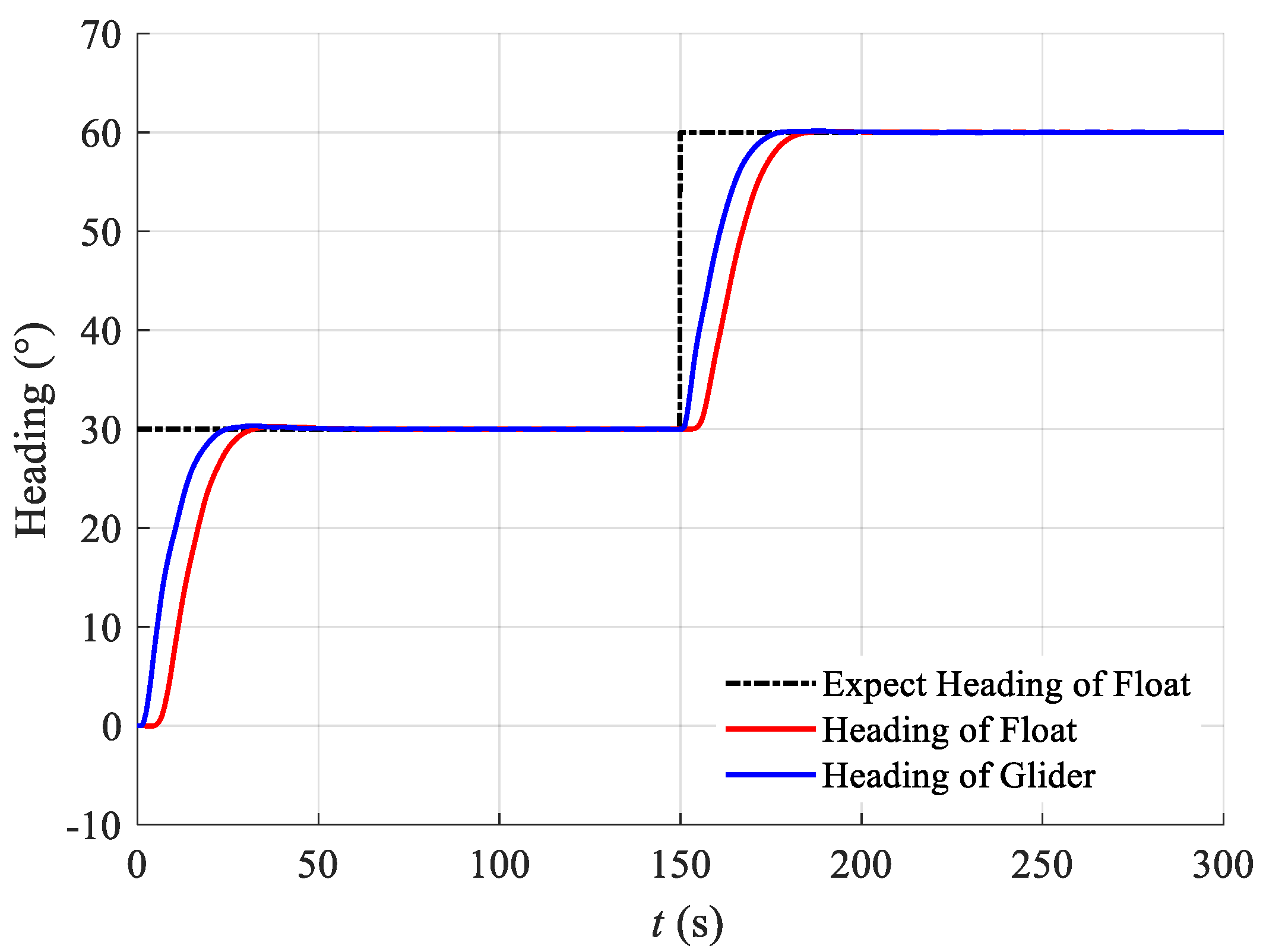
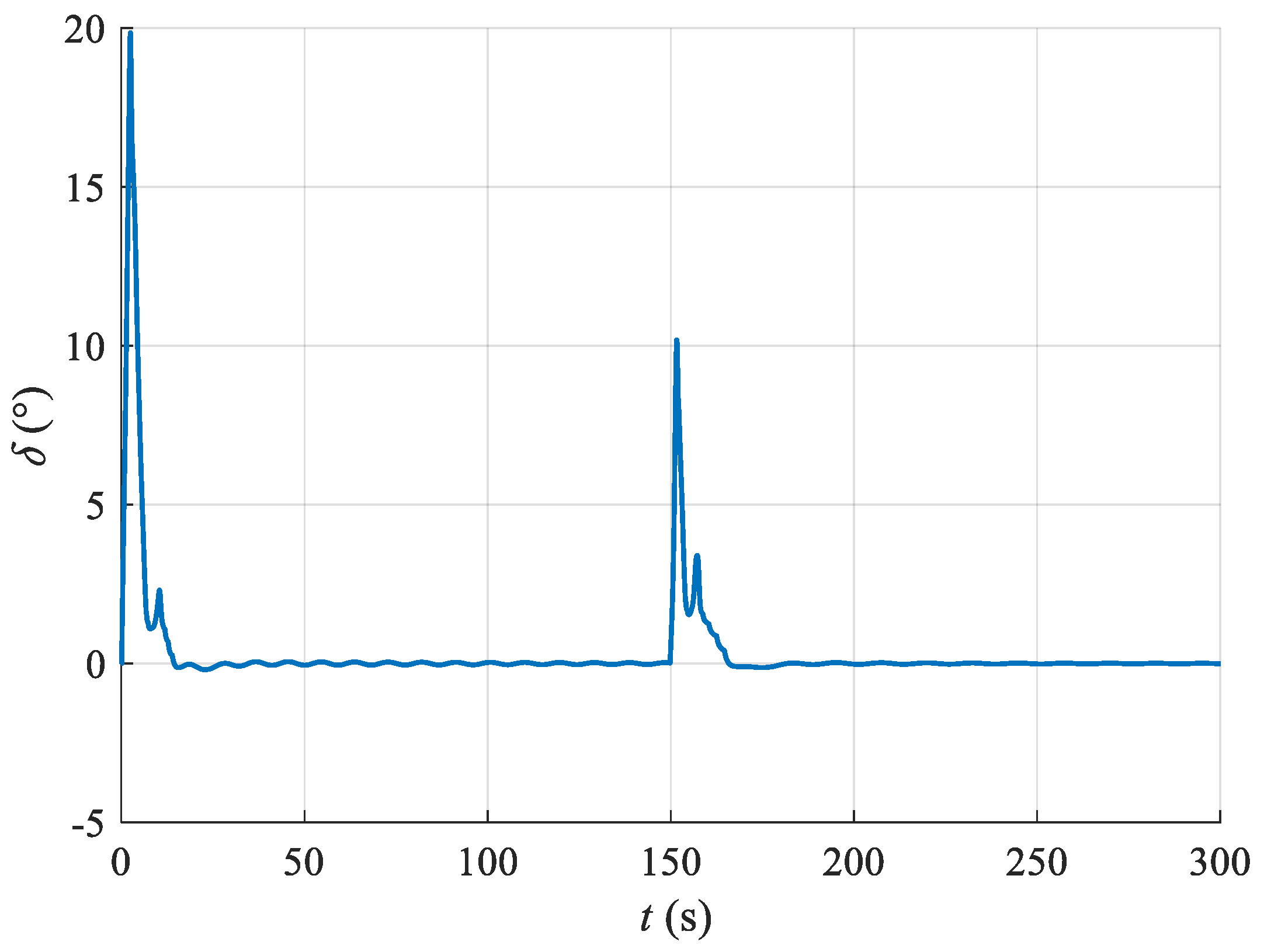
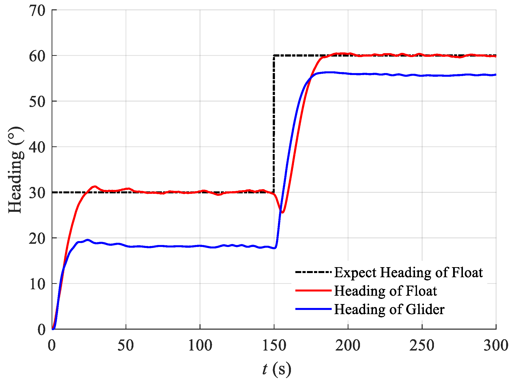
5.1. Float Heading Control Simulation

To simulate a real ocean environment, in order to simulate the real marine environment, the current marine environment was set as the second level of the sea state, in which the wave height should be set to 0.3 m and the wavelength should be set to 8 m. The initial heading of both the floater and the submersible was 0°. The desired heading of the floater was set to 30° for the first 150 s and 60° for the next 150 s. The controller parameters were set as follows: $\lambda =0.1$, $\eta =0.1$, $k_r=10$, $\mu =0.6$, $\kappa =0.3$. The floating weight of the wave glider was 55 kg, the mass of the submerged body was 40, and the moments of inertia were 90, 10, and 10, respectively. And the discrete time was set to 0.01. The simulation results of the floater and submersible heading, as well as the rudder angle, are shown in Figure 4 and Figure 5.

From Figure 4, it can be observed that the submersible responds first. When there is a heading difference between the float and the submersible, the float receives the control input. The time to reach stability is approximately 24 s. After stabilization, due to external waves and other real environmental factors, the floater exhibits oscillations within 0.2°. From Figure 5, it can be seen that the output oscillation is within 0.15°, which indicates that stable control has been achieved. After 150 s, the desired heading of the float is switched. Similarly, the submersible responds first, and after a heading difference arises between the submersible and the float, the float receives the control input, and its heading begins to respond. The time to reach stability is approximately 28 s. At this point, the float’s oscillation is within 0.15°, and the control output oscillation is within 0.10°, indicating that control stability has been achieved.

To verify the disturbance resistance of the heading control algorithm and better simulate the real environment, while maintaining the same simulation conditions as the above experiment, a heading disturbance torque was applied to the floater as follows:

$$M_d=\left\{\begin{array}{l}\begin{array}{ccc}(0.5+2·\mathrm{randn})\mathrm{N}\cdot \mathrm{m}& & 0\mathrm{s}<t\le 150\mathrm{s}\end{array}\\ \begin{array}{ccc}(-0.5+2·\mathrm{randn})\mathrm{N}\cdot \mathrm{m}& & 150\mathrm{s}<t<300\mathrm{s}\end{array}\end{array}\right.$$

The disturbance was a combination of steady disturbance and random disturbance. The simulation results at this time are shown in Figure 6 and Figure 7.

From Figure 6, it can be seen that when the DMFAC float heading controller is used to control the floater, due to the initial application of a positive torque on the floater, the floater begins to respond right from the start. During the first 150 s, the heading stabilizes in about 25 s, with a maximum overshoot of approximately 1.1°. Afterward, the heading control stabilizes. Due to external disturbances such as waves, there is a stable heading difference between the submersible and the floater, which helps resist external disturbances. Although there is slight oscillation after stabilization, the oscillation amplitude is within 0.5°. From the analysis of Figure 7, it can be concluded that the control output oscillation is within 0.2°, indicating good stability. After 150 s, the floater’s desired heading is switched, and the direction of the heading disturbance applied to the floater is also reversed. As a result, the floater turns slightly in the opposite direction, with a maximum rotation angle of about 4.6°. It takes 34 s to reach stability again, with a maximum overshoot of approximately 0.58°. Similarly, due to external disturbances, there is a stable heading difference between the submersible and the floater, and the oscillation amplitude remains within 0.5°. From Figure 7, it can be concluded that the control output oscillation is also within 0.2° at this time. A detailed comparison of the data is shown in

Table 1. Comparison of heading simulation with and without disturbance.

	Heading Overshoot	Maximum Heading Oscillation	Maximum Rudder Angle Oscillation
With disturbance	/	0.2°	0.1°
Without disturbance	1.1°	0.5°	0.2°

. Therefore, it can be concluded that the floater heading control has achieved good disturbance resistance.

5.2. Wave Glider Mooring Control Simulation

In setting the ocean environment with a wave height of 0.3 m and a wavelength of 8 m, the UWG path points were set as follows: (−200, 100), (200, 50), and (400, −200), with the mooring point being the final destination (400, −200). The initial position of the UWG was (−100, 50), and the attraction range of the mooring point was 15 m. The path-following phase is shown in Figure 8, and the mooring phase is shown in Figure 9:

The green line in Figure 9 represents the anchoring circle, with the anchorage point as the center and the anchorage distance as the radius. When the UWG is within this anchoring circle, it indicates that the anchoring requirements are met. From Figure 8, it can be observed that when the UWG uses IAFLOS for path following, the overshoot is relatively small, at 4.95 m, and the turns are smooth without any overshoot. Upon reaching the mooring point, no control is applied within a 10 m radius of the mooring point. If the UWG exceeds this 10 m radius, an attractive force toward the mooring point is applied, ensuring that the UWG remains near the mooring point. To quantitatively analyze the control process, the lateral error during the path-following phase and the distance from the mooring point during the mooring phase are shown in the simulation graphs in Figure 10 and Figure 11.

From Figure 10, it can be seen that the UWG reaches the mooring point at around 1600 s. During the path-following process, the maximum path overshoot is 4.96 m, and no overshoot occurs when switching paths. After reaching tracking stability, no oscillations are observed. From Figure 11, it can be seen that after reaching the mooring point, the distance between the UWG and the mooring point is controlled within 20 m, with the maximum distance being 15.98 m, which meets the requirements of the set mooring control.

Next, to better simulate the ocean environment and the noise disturbances encountered in real-world situations, and to verify the disturbance resistance of the algorithm, the floater heading and heading control simulation were set as follows:

$$M_d=(1+2·\mathrm{randn})\mathrm{N}\cdot \mathrm{m}$$

The simulation results are shown in Figure 12 and Figure 13.

The meaning of the green line in the figure is consistent with what was described earlier in the text. From Figure 12 and Figure 13, it can be seen that even under applied disturbances, the UWG is still able to complete the path-following and mooring processes successfully, without significant overshoot or severe oscillations, demonstrating the algorithm’s strong disturbance resistance. Additionally, a path-tracking error simulation and mooring distance simulation during the mooring phase in Figure 14 and Figure 15 were performed to better conduct a quantitative analysis:

From Figure 14 and Figure 15, it can be seen that after adding disturbances, the maximum overshoot during the path-following phase reached 5.03 m, which is only 0.08 m more than in the absence of disturbances. Although oscillations within the 0.1 m range occurred after stable tracking, the control accuracy requirements were still met. In the mooring phase, only during the initial mooring stage around 1750 s did the distance from the mooring point reach a maximum of 19.5 m, while during the rest of the time, the maximum distance from the mooring point was 16.7 m, meeting the mooring accuracy requirements. This set of simulation results verify that the proposed algorithm can meet the UWG mooring tracking control requirements under external disturbances and real sea conditions. A comparison of the simulation data under the two types of disturbances is shown in

Table 2. Comparison of path-following data with and without disturbances.

	Maximum Path Overshoot	Maximum Distance from the Mooring Point	Average Path-Following Error
With disturbances	5.03 m	19.50 m	3.98 m
Without Disturbances	4.95 m	15.98 m	4.24 m

:

6. Conclusions

This paper, focusing on UWG fixed-point mooring control, discusses the floater heading control and mooring process strategy of the UWG. This study explored the UWG floater heading control based on DMFAC and the mooring process strategy based on IAFLOS, followed by simulation studies. The main conclusions are as follows:

(1)

Due to the presence of many unknown nonlinear terms and time delay terms in the UWG floater heading control system, MFAC cannot be directly applied to the floater heading control system. Therefore, this paper introduces differential terms into the criterion function and designed the DMFAC floater heading control method, proving the stability of the control algorithm. This allows the heading control subsystem to match the dynamic change speed of MFAC, solving the problems of oscillation and non-convergence in standard MFAC methods for UWG heading control.

(2)

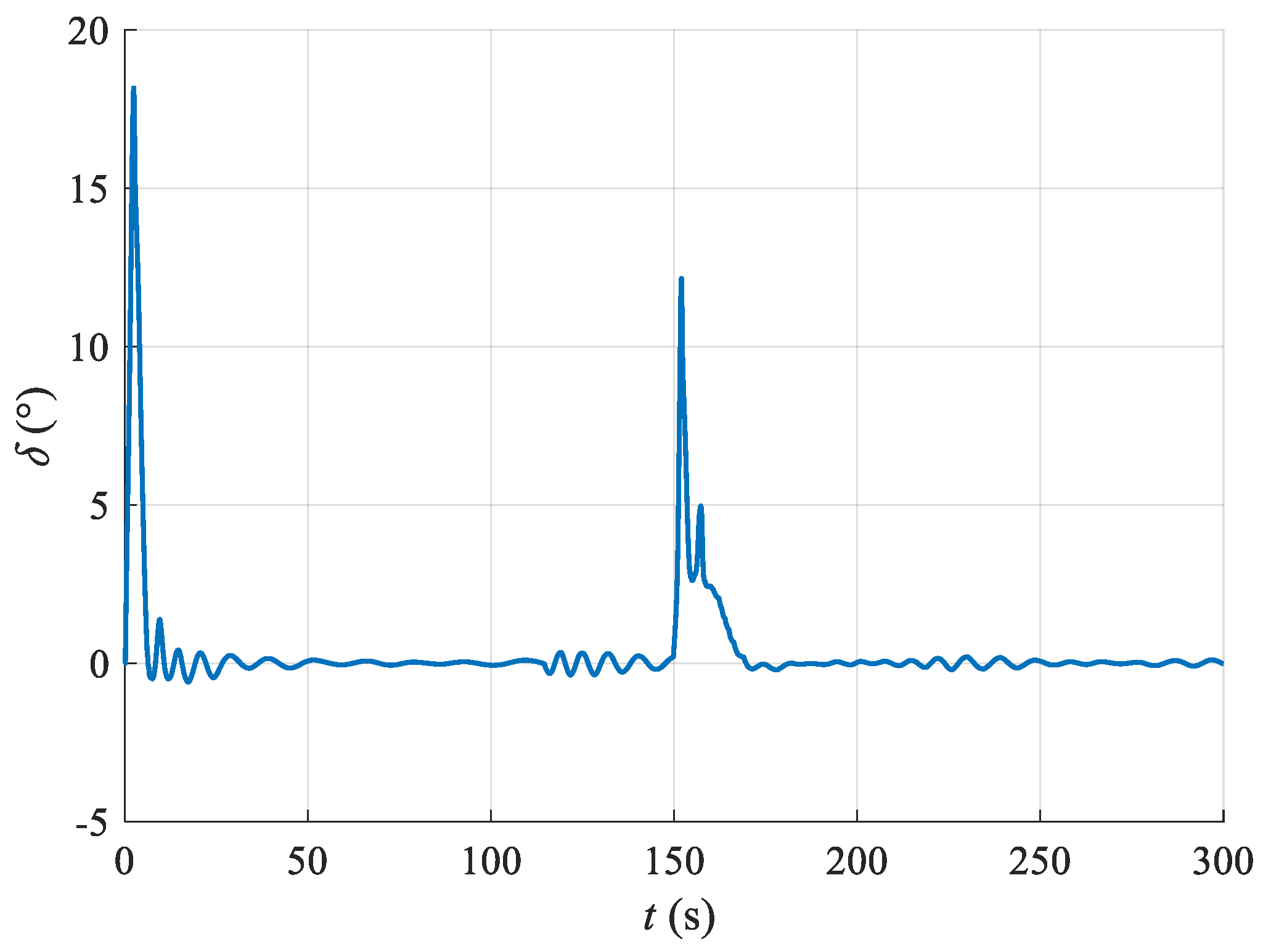
The simulations demonstrated that the designed UWG heading control method can achieve good stability while also exhibiting strong disturbance resistance. The simulation results show that under simulated Beaufort scale 2 sea conditions, in the absence of disturbances, the final heading control error is within 0.1°, and with disturbances applied, the UWG heading control fluctuates within 0.6°, reflecting the excellent disturbance resistance of the heading control system.

(3)

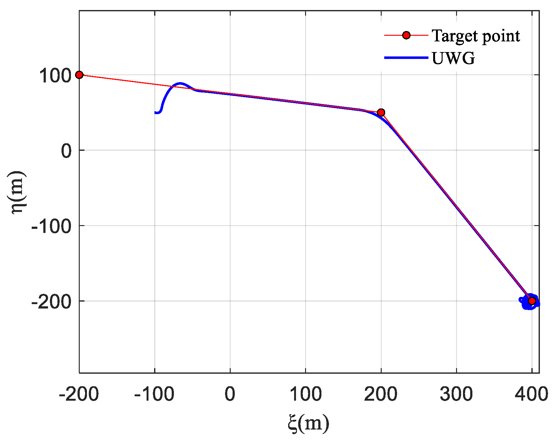
Considering that a UWG, as a vehicle with weak maneuverability and significant wave influence, may experience control failure when using LOS for path-following control, the IAFLOS path-following and mooring control strategies were designed. The aim was to ensure the successful completion of the mooring process without failure by designing different attractive force terms, while also reducing control overshoot.

(4)

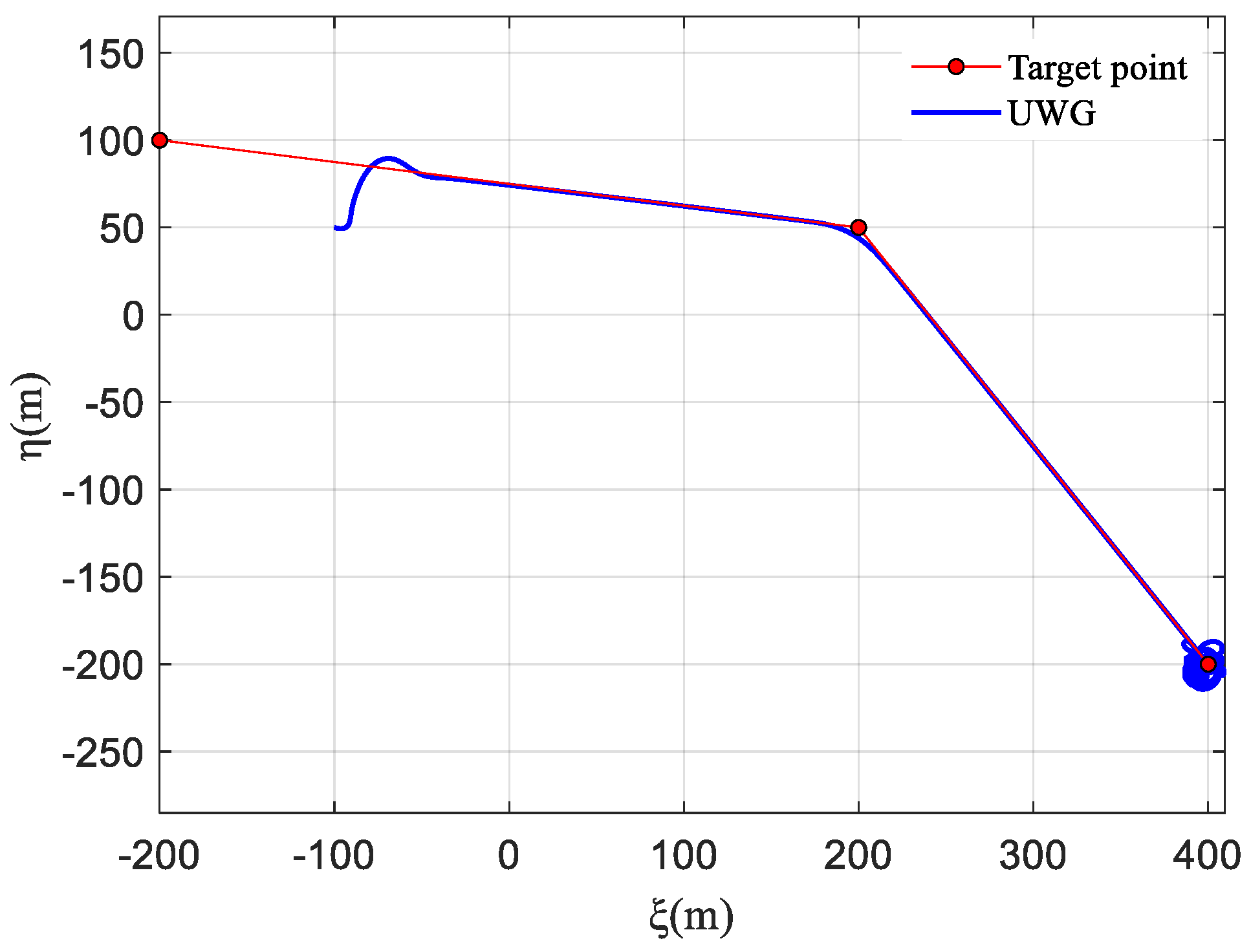
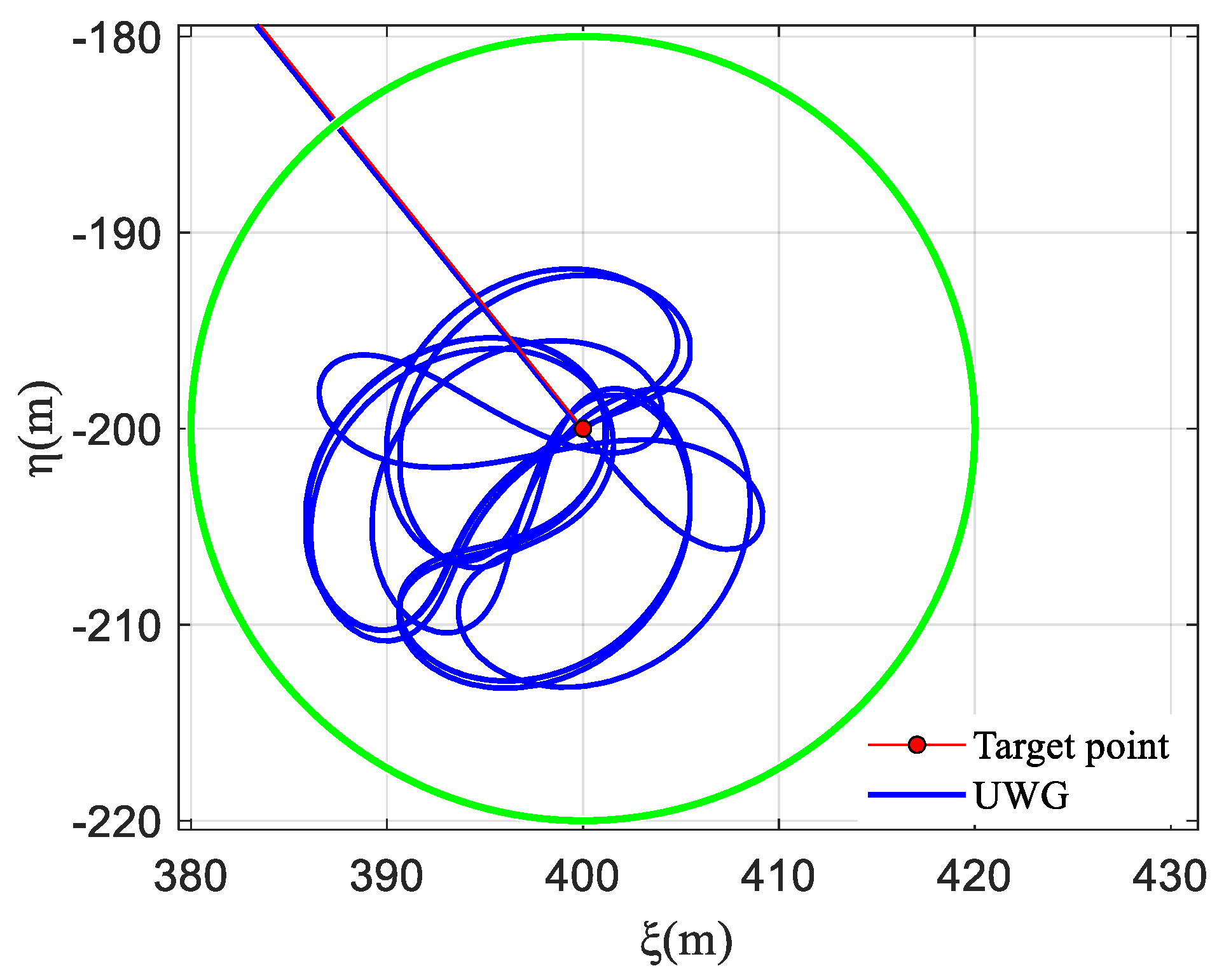
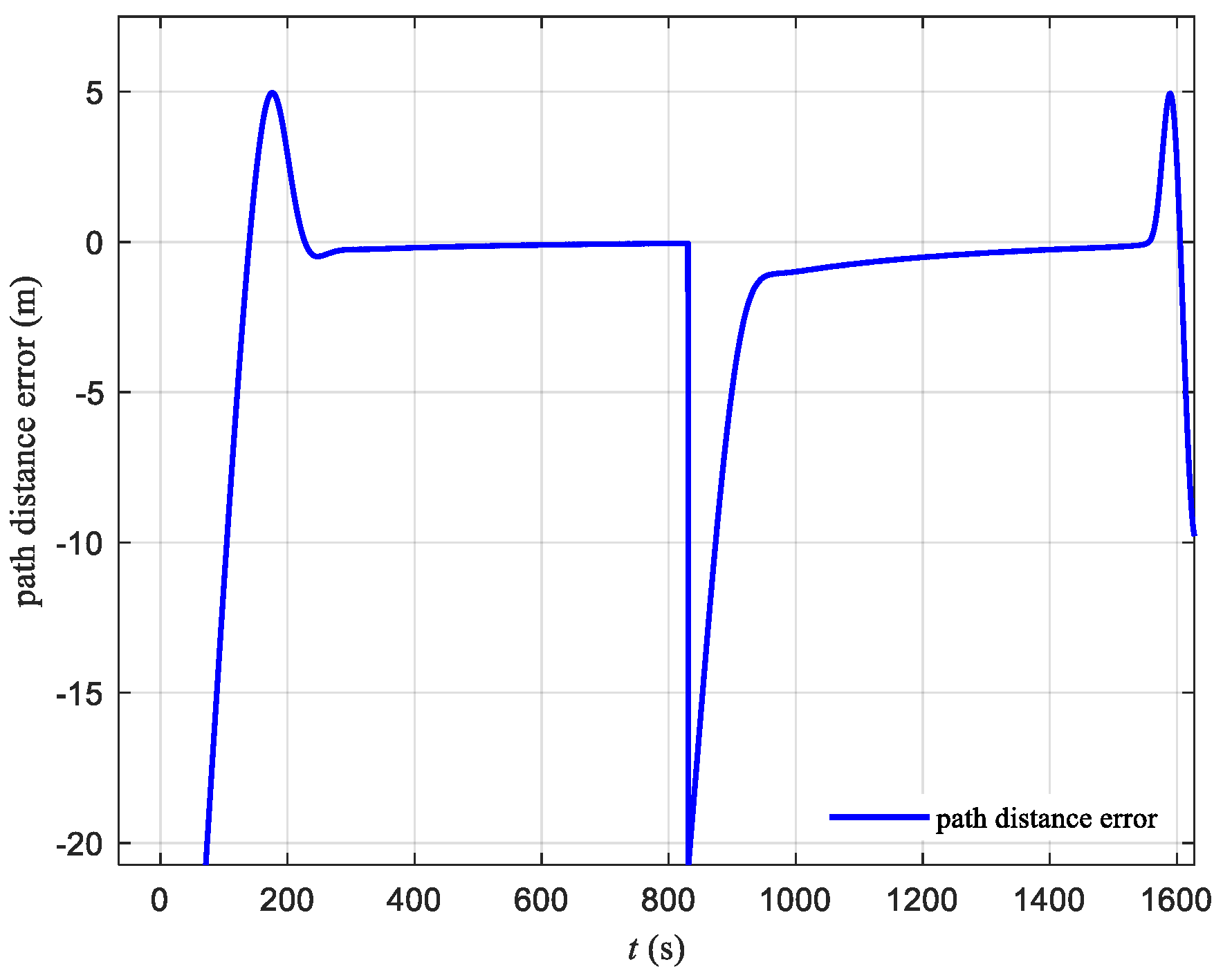
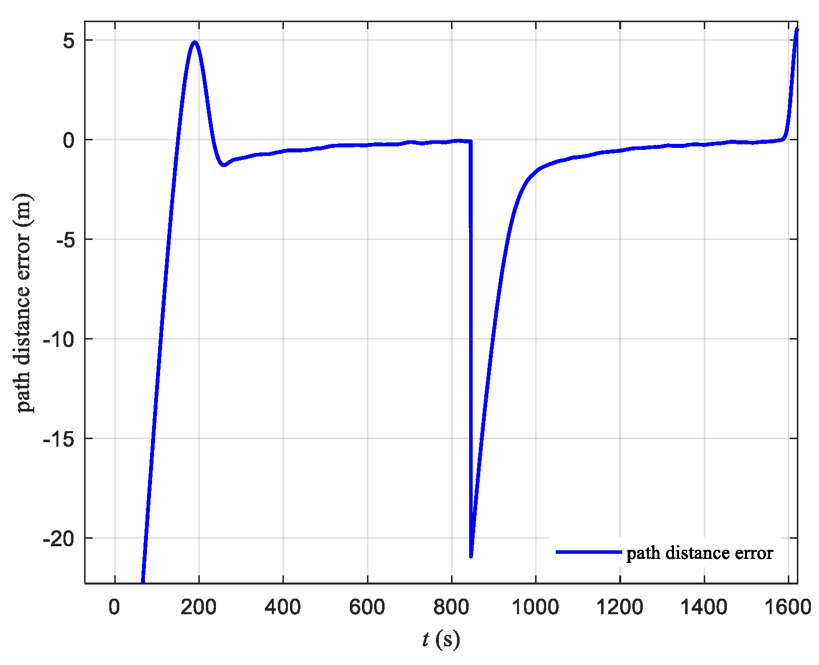
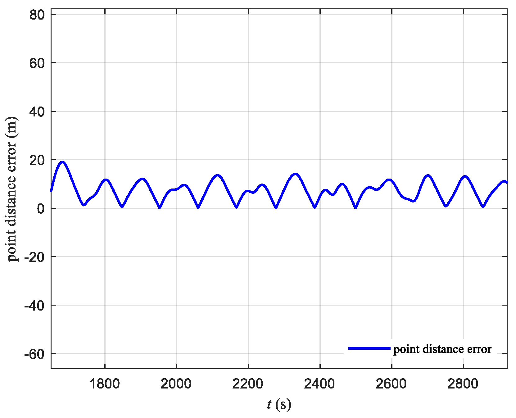
The simulation verified that the designed mooring control strategy can achieve good path-following and mooring control under Beaufort scale 2 sea conditions. Without disturbances, the maximum overshoot is 4.95 m, and after stabilization, the path oscillation is almost 0. With disturbances applied, the maximum overshoot is 5.03 m, and after stabilization, the path oscillation is within 0.1 m. During the mooring phase, whether with or without disturbances, the maximum distance from the mooring point is controlled within 20 m, meeting the requirements of the mooring control task.

References

1. Manley, J.; Willcox, S. The Wave Glider: A New Concept for Deploying Ocean Instrumentation. IEEE Instrum. Meas. Mag. 2010, 13, 8–13. [Google Scholar] [CrossRef]
2. Zhou, H.; Xu, H.; Cao, J.; Fu, J.; Mao, Z.; Zeng, Z.; Yao, B.; Lian, L. Robust Adaptive Control of Underwater Glider for Bottom Sitting-Oriented Soft Landing. Ocean Eng. 2024, 293, 116725. [Google Scholar] [CrossRef]
3. Bi, Y.; Jin, Y.; Zhou, H.; Bai, Y.; Lyu, C.; Zeng, Z.; Lian, L. Surfing Algorithm: Agile and Safe Transition Strategy for Hybrid Aerial Underwater Vehicle in Waves. IEEE Trans. Robot. 2023, 39, 4262–4278. [Google Scholar] [CrossRef]
4. Thomson, J.; Girton, J.B.; Jha, R.; Trapani, A. Measurements of Directional Wave Spectra and Wind Stress from a Wave Glider Autonomous Surface Vehicle. J. Atmos. Ocean. Technol. 2018, 35, 347–363. [Google Scholar] [CrossRef]
5. Fu, J.; Zhou, H.; Zhang, X.; Wen, H.; Yao, B.; Lian, L. A Unified Switching Dynamic Modeling of Multi-Mode Underwater Vehicle. Ocean Eng. 2023, 278, 114359. [Google Scholar] [CrossRef]
6. Li, Y.; Pan, K.; Liao, Y.; Zhang, W.; Wang, L. Improved Active Disturbance Rejection Heading Control for Unmanned Wave Glider. Appl. Ocean Res. 2021, 106, 102438. [Google Scholar] [CrossRef]
7. Berger, J.; Laske, G.; Babcock, J.; Orcutt, J. An Ocean Bottom Seismic Observatory with near Real-Time Telemetry. Earth Space Sci. 2016, 3, 68–77. [Google Scholar] [CrossRef]
8. Mitarai, S.; McWilliams, J.C. Wave Glider Observations of Surface Winds and Currents in the Core of Typhoon Danas. Geophys. Res. Lett. 2016, 43, 11312–11319. [Google Scholar] [CrossRef]
9. Peng, Z.; Li, J.; Han, B.; Gu, N. Safety-Certificated Line-of-Sight Guidance of Unmanned Surface Vehicles for Straight-Line Following in a Constrained Water Region Subject to Ocean Currents. J. Mar. Sci. Appl. 2023, 22, 602–613. [Google Scholar] [CrossRef]
10. Abrougui, H.; Nejim, S. Autopilot Design for an Unmanned Surface Vehicle Based on Backstepping Integral Technique with Experimental Results. J. Mar. Sci. Appl. 2023, 22, 614–623. [Google Scholar] [CrossRef]
11. Zhou, H.; Cao, J.; Fu, J.; Zeng, Z.; Yao, B.; Mao, Z.; Lian, L. Swift: Transition Characterization and Motion Analysis of a Multimodal Underwater Vehicle. IEEE Robot. Autom. Lett. 2024, 9, 1692–1699. [Google Scholar] [CrossRef]
12. Wang, P.; Wang, D.; Zhang, X.; Guo, X.; Li, X.; Tian, X. Path Following Control of the Wave Glider in Waves and Currents. Ocean Eng. 2019, 193, 106578. [Google Scholar] [CrossRef]
13. Li, Y.; Pan, K.; Liao, Y.; Zhang, W.; Wang, L. Dynamics Modeling and Experiments of Wave Driven Robot. Appl. Math. Model. 2020, 79, 451–468. [Google Scholar] [CrossRef]
14. Shi, Y.; Shen, C.; Fang, H.; Li, H. Advanced Control in Marine Mechatronic Systems: A Survey. IEEE-ASME Trans. Mechatron. 2017, 22, 1121–1131. [Google Scholar] [CrossRef]
15. Yuan, J.; Zhang, W.; Liu, H.; Li, H. Heading and Speed Joint Control of Double-Push Usv Based on Fuzzy Pid. Int. J. Robot. Autom. 2023, 38, 32–41. [Google Scholar] [CrossRef]
16. Shin, H.; Baek, S.; Song, Y. Multidimensional Beam Optimization in Underwater Optical Wireless Communication Based on Deep Reinforcement Learning. IEEE Internet Things J. 2024, 11, 28623–28634. [Google Scholar] [CrossRef]
17. Wu, C.; Yu, W.; Liao, W.; Ou, Y. Deep Reinforcement Learning with Intrinsic Curiosity Module Based Trajectory Tracking Control for USV. Ocean Eng. 2024, 308, 118342. [Google Scholar] [CrossRef]
18. Zhang, X.; Zhou, H.; Fu, J.; Wen, H.; Yao, B.; Lian, L. Adaptive Integral Terminal Sliding Mode Based Trajectory Tracking Control of Underwater Glider. Ocean Eng. 2023, 269, 113436. [Google Scholar] [CrossRef]
19. Jia, Q.; Liao, Y.; Xu, P.; Pang, S.; Wang, B.; Li, Y. Modeling Analysis and Experiment for Energy System of Ocean Energy Driven Unmanned Marine Vehicle: The Yulang II Case Study. J. Field Robot. 2024, 41, 735–765. [Google Scholar] [CrossRef]
20. Zhang, J.; Zhang, W.; Tong, S. Adaptive Neural Optimal Tracking Control for Uncertain Unmanned Surface Vehicle. Ocean Eng. 2024, 312, 119031. [Google Scholar] [CrossRef]
21. Lei, T.; Wen, Y.; Yu, Y.; Tian, K.; Zhu, M. Predictive Trajectory Tracking Control for the USV in Networked Environments with Communication Constraints. Ocean Eng. 2024, 298, 117185. [Google Scholar] [CrossRef]
22. Fan, Y.; Qiu, B.; Liu, L.; Yang, Y. Global Fixed-Time Trajectory Tracking Control of Underactuated USV Based on Fixed-Time Extended State Observer. ISA Trans. 2023, 132, 267–277. [Google Scholar] [CrossRef] [PubMed]
23. Chen, C.; Liao, Y.; Tang, X.; Sun, J.; Gu, J.; Li, H.; Ren, Z.; Zhai, Z.; Li, Y.; Wang, B.; et al. Research on double-USVs fuzzy-priority NSB behavior fusion formation control method for oil spill recovery. J. Field Robot. 2024, 41, 1–25. [Google Scholar] [CrossRef]
24. Liao, Y.; Chen, C.; Du, T.; Sun, J.; Xin, Y.; Zhai, Z.; Wang, B.; Li, Y.; Pang, S. Research on disturbance rejection motion control method of USV for UUV recovery. J. Field Robot. 2023, 40, 574–594. [Google Scholar] [CrossRef]
25. Yu, P.; Zhou, Y.; Sun, X.; Sang, H.; Zhang, S. Adaptive Path Following Control for Wave Gliders in Ocean Currents and Waves. Ocean Eng. 2023, 284, 115251. [Google Scholar] [CrossRef]
26. Zhang, S.; Sang, H.; Sun, X.; Liu, F.; Zhou, Y.; Yu, P. Research on Path Following Control System of Wave Gliders Based on Maneuverability Demand Estimator. Ocean Eng. 2023, 287, 115932. [Google Scholar] [CrossRef]
27. Qi, Z.; Wang, B.; Qin, Y.; Shi, J.; Zhai, J. Planar Path Following Control for Wave Glider and Experimental Study. J. Coast. Res. 2020, 99, 16–20. [Google Scholar] [CrossRef]
28. Zhang, S.; Sang, H.; Sun, X.; Liu, F.; Zhou, Y.; Yu, P. Research on the Maneuverability and Path Following Control of the Wave Glider with a Propeller-Rudder System. Ocean Eng. 2023, 278, 114346. [Google Scholar] [CrossRef]
29. Liu, R.; Tian, X.; Wang, P.; Liao, N.; Huang, R.; Xu, H.; Wang, F. Experimental-Based Hydrodynamic Simulation of Submarine Glider for Wave Gliders. Appl. Ocean Res. 2024, 153, 104224. [Google Scholar] [CrossRef]
30. Wang, P.; Tian, X.; Lu, W.; Hu, Z.; Luo, Y. Dynamic Modeling and Simulations of the Wave Glider. Appl. Math. Model. 2019, 66, 77–96. [Google Scholar] [CrossRef]
31. Hou, Z.; Jin, S. A Novel Data-Driven Control Approach for a Class of Discrete-Time Nonlinear Systems. IEEE Trans. Control Syst. Technol. 2011, 19, 1549–1558. [Google Scholar] [CrossRef]
32. Hou, Z.; Chi, R.; Gao, H. An Overview of Dynamic-Linearization-Based Data-Driven Control and Applications. IEEE Trans. Ind. Electron. 2017, 64, 4076–4090. [Google Scholar] [CrossRef]
33. Hou, Z.; Jin, S. Data-Driven Model-Free Adaptive Control for a Class of MIMO Nonlinear Discrete-Time Systems. IEEE Trans. Neural Netw. 2011, 22, 2173–2188. [Google Scholar] [PubMed]
34. Hou, Z.; Jin, S. Model Free Adaptive Control: Theory and Applications; CRC Press: Boca Raton, FL, USA; Taylor & Francis Group: Oxfordshire, UK, 2013. [Google Scholar]
Figure 1. UWG’s principles of movement.
Jmse 12 02282 g001
Figure 2. UWG coordinate system.
Jmse 12 02282 g002
Figure 3. IAFLOS schematic.
Jmse 12 02282 g003
Figure 4. Simulated heading response curve of the submersible and float.
Jmse 12 02282 g004
Figure 5. Simulated rudder angle of the submersible.
Jmse 12 02282 g005
Figure 6. Simulated heading response curve of the submersible and floater.
Jmse 12 02282 g006
Figure 7. Simulated rudder angle of the submersible.
Jmse 12 02282 g007
Figure 8. UWG path-following phase.
Jmse 12 02282 g008
Figure 9. UWG mooring phase.
Jmse 12 02282 g009
Figure 10. Path-following phase path error simulation.
Jmse 12 02282 g010
Figure 11. Simulation of mooring distance during mooring phase.
Jmse 12 02282 g011
Figure 12. UWG path-following phase.
Jmse 12 02282 g012
Figure 13. Mooring phase simulation.
Jmse 12 02282 g013
Figure 14. UWG path-following phase.
Jmse 12 02282 g014
Figure 15. Simulation of mooring distance during mooring phase.
Jmse 12 02282 g015