Article

Satellite Altimetry and Seasonal Circulation in the Ligurian Sea

1
Hydrographic Institute, 16135 Genoa, Italy
2
Department of Civil, Chemical and Environmental Engineering (DICCA), University of Genoa, 16126 Genoa, Italy
3
Institute of Biophysics, National Research Council (CNR), 56124 Pisa, Italy
*
Author to whom correspondence should be addressed.
J. Mar. Sci. Eng. 2024, 12(12), 2281; https://doi.org/10.3390/jmse12122281
Submission received: 28 October 2024 / Revised: 5 December 2024 / Accepted: 10 December 2024 / Published: 11 December 2024
(This article belongs to the Section Physical Oceanography)

Abstract

:
Satellite altimetry observations are checked against in situ measurements to assess the capability of this remote sensing technique to describe the surface circulation in the Ligurian Sea. CTD profiles were collected during five oceanographic campaigns from 2017 and 2024 along the satellite track Jason 044, crossing the Ligurian Sea from the Corsica Channel to the coast close to Genoa. Eight months of ADCP surface currents from a fixed mooring were also used for the comparison with altimetric-derived geostrophic currents. Moreover, the possible contribution of ICESat-2 to oceanographic studies in the area is investigated. Altimetric measurements successfully reproduce the basic circulation features of the region and their seasonal variation and, despite the different nature of the used systems, can be well integrated with in situ observations. The results from the direct comparison with daily mean values of ADCP surface currents reported an RMSD of the same order as the standard deviation, which is consistent with similar investigations in other areas but evidences the need to define more appropriate metrics and methods.

1. Introduction

Satellite observations have proven to be a powerful tool to increase the scientific knowledge of oceanographic and dynamic processes, particularly in areas where in situ measurements are scarce [1]. The investigation of large current systems has strongly benefited from satellite altimetry (e.g., see [2] for a review). The accuracy now achieved by satellite altimetry observations allows for approaching ocean dynamics studies even in those regions, such as the Mediterranean Sea, where the surface signature related to the ocean circulation is generally low [3,4,5,6], and the presence of islands and complex topography can affect the quality of the measurements.
Several research studies have highlighted the usefulness of satellite altimetry in supporting oceanographic studies in this area. For instance, satellite altimetry allowed for the correlation of the dynamic height differences between the Ligurian and the Tyrrhenian Seas with the climatological CTD computed dynamic height, as well as the water exchange across the Corsica Channel [7,8]. The integration of gliders with altimeters to understand mesoscale variability was among the main objectives of more recent experiments [9,10].
One of the objectives of this study is to assess the capability of satellite altimeter observations to be combined with in situ measurements to support the studies of surface circulation in the region. To this end, a series of CTD casts along the ground track 044 of the reference altimeters missions (TOPEX/Poseidon, Jason 1/2/3 and Sentilnel-6), crossing the Central Ligurian Sea from 43.15° N; 9.78° E to 44.33° N; 8.79° E, as well as near-surface ADCP currents from a fixed mooring located mid-way on the track, are considered for this analysis.
The selected track, starting South of Elba Island, moves northwest, crossing the Ligurian Sea up to the coast close to Genoa. It follows the part of the Ligurian-Provençal Current quite closely, which moves to the north, separating the deep western side of the Ligurian Sea with its large cyclonic system from the shallow eastern side of the Ligurian Sea. The bottom topography along the track is quite complex (Figure 1). In the southern part, the track follows the eastern side of the Corsica Channel, passing over Capraia Island. Moving to the north, it separates the shelf area with the Tuscan Archipelago at the eastern side, while the west opens the deep basin. Approaching the Ligurian coasts, the bottom is modified by two deep canyons north–south oriented in front of Genoa and one along-shore oriented at the east [11].
The complex topography, the presence of different water masses, and the influence of different meteorological conditions can generate relevant mesoscale activity even over short time and space scales [12,13]. That is why there is a need to assess and validate multiplatform observation approaches.

2. Data and Methods

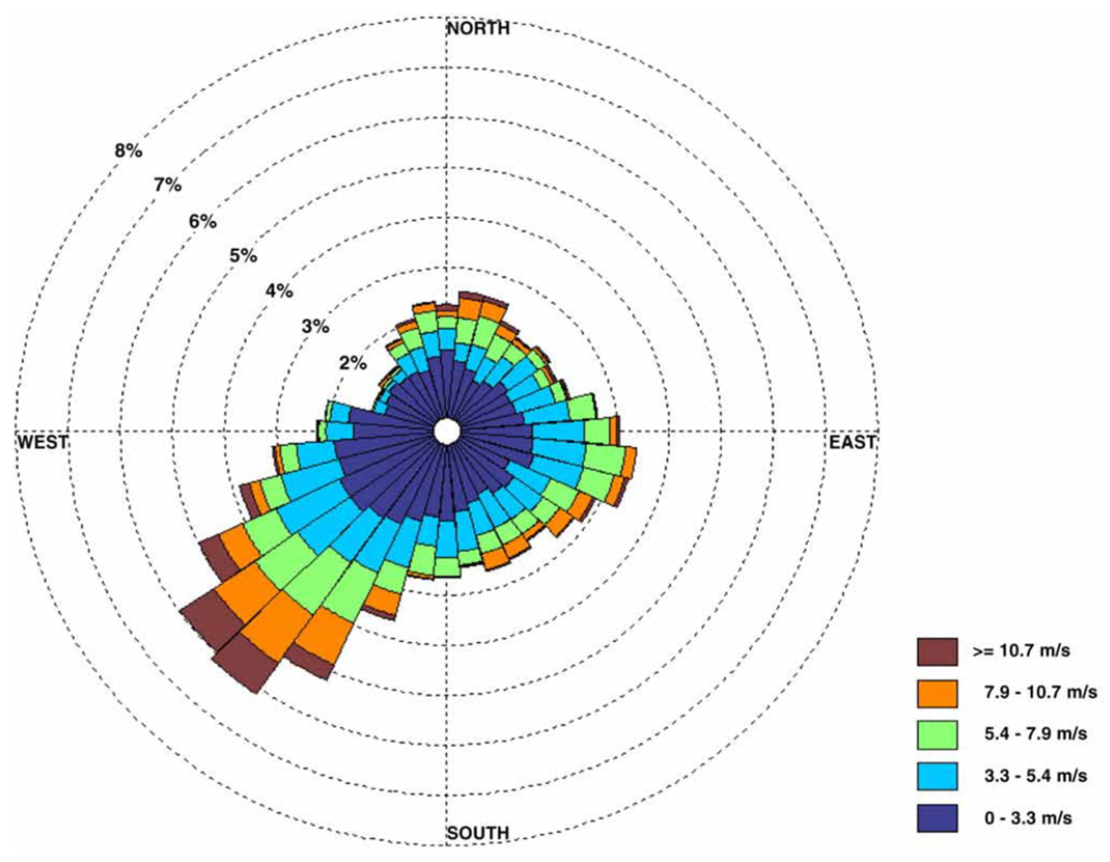
2.1. Meteorological and Oceanographic Setting of the Ligurian Sea

The Ligurian Sea occupies the northwestern part of the Mediterranean Sea and is a 3000 m deep basin opening to the southwest with a narrow and deep shelf that flattens at the eastern edge. The connection with the Tyrrhenian Sea occurs through the Corsica Channel, a narrow sill with a maximum depth of about 450 m. The Ligurian Sea, and the Gulf of Genoa in particular, is one of the most active areas of cyclogenesis in the Mediterranean [14,15], often responsible for heavy rain and storms. Winds regime is characterized by Tramontana (N), Scirocco (SW), and Libeccio (SW), the first one prevailing during winter, the last one associated with the strongest storms [16,17,18]. Climatological maps of wind waves estimation in the Mediterranean Sea based on ERA5 reanalysis and WAVEWATCH III [19] report values of 50% Hs in the range of 0.6–1 m during winter and 0.3–0.6 m during summer and extremes (99% Hs) up to 4 m in winter and 2 m in summer along the investigated track. Maximum individual wave heights are, respectively, 2.2 m and 8 m for winter and 1 m and 6 m for summer. Measurements from a wave-gauge buoy deployed far from the Gulf of La Spezia [20] and resumed in the form of a wind rose to indicate that the waves from Libeccio were by far stronger than the others. The most damaging wave storms in the Gulf of Genoa are also generated by Libeccio winds, despite those from Scirocco occurring more frequently [21]. See Figure 2.
The tidal regime is semi-diurnal, but tides are quite small in the area: M2, the dominant component, has an amplitude of 8.5 cm; K1, the highest diurnal component, is only 3.5 cm [22].
Since the pioneering works of the 1960s [23,24], the circulation of this basin has been widely investigated and, due to its economic and environmental importance, is still the object of several studies. A recent and exhaustive review can be found in [25]. As a part of the Mediterranean Sea, the circulation in the Ligurian Sea is related to the large-scale circulation of this basin, but it is also strongly modified by the local meteorological, climatic, and topographic conditions. Surface (Modify Atlantic Water—MAW) and intermediate (Levantine Intermediate Waters—LIW) water masses characterizing the whole Mediterranean Sea can still be detected despite the long travel from Gibraltar to the eastern Mediterranean and back. In particular, the presence of the LIW can be well identified in the temperature and salinity profiles of the Ligurian Sea by a relative maximum of temperature and salinity located around 400 m depth, with typical values of 13.9 °C and 38.6. What remains of the MAW can be tracked in the surface layer as a relative minimum of salinity (37.9) at about 40 m, but it can be masked during winter by strong mixing events [26,27,28]. On the contrary, due to the topographic constraints (Sicily, Sardinia, and Corsica Channels) that separate the deep parts of the Eastern and Western Mediterranean sub-basins, the deep circulation is generated locally under the influence of peculiar climatic conditions. The colder and denser deep waters (Western Mediterranean Deep Water—WMDW), with temperature and salinity values around 12.8 °C and 38.46, are formed during winter in the Northern part of the Ligurian Provencal basin as the results of strong convective events generated by Mistral and Tramontana winds [29,30].
The Ligurian Sea circulation, characterized by a large cyclonic gyre that occupies the central part of the basin, involves both surface waters and LIW. This main current system, the Ligurian Provencal Current (LPC), is fed by the Western Corsica Current (WCC) and the Eastern Corsica Current (ECC), two current systems flowing along the western and the eastern coasts of the Corse, which merge north of Cape Corse. These two currents are characterized by differences in the water properties, with ECC being warmer and saltier than WCC [31]. LPC or Northern Current (NC) flows along the Ligurian and French coasts [32,33,34]. The cyclonic circulation is generally intensified during winter, but the surface circulation can be affected by the transit of low-pressure systems [35]. In the shallow eastern part, the circulation has a higher variability and is characterized by a weak anticyclonic gyre—the Ligurian Anticyclone (LA)—more frequent during summer, whose position can shift from the north of the Elba island to the coastal region of the Gulf of La Spezia [36,37,38].

2.2. SWIM-LIG Campaigns

During a joint oceanographic campaign with the NATO Centre for Marine Research and Experimentation (CMRE) in late summer 2017, in the framework of the project LOGMEC17, the ITS Aretusa of the Italian Navy performed a long transect from Montecristo Island to Genova collecting data with XBTs and CTDs probe. The idea was to obtain oceanographic data along route number 44 of the Jason satellite to compare them with the altimetry data of the satellite.
This part of the campaign, named ARET17, revealed the full potentiality of collecting reliable data and the opportunity to plan a more regular sort of oceanographic monitoring, which was the obvious conclusion. It was then decided to plan two campaigns each year—one in winter and one at the end of summer, with the aim of maintaining regular monitoring of the Ligurian Sea as a support to environmental, climatic, and air–sea interaction studies in this area. The same monitoring scheme of CNR campaigns carried out in September 2015 and April 2017 in the framework of EU project FixO3 [39] was chosen, which includes five coast-open sea transects in the Eastern and Central Ligurian Sea and, when possible, a piece of the Jason 044 track was added.
The longest route along the Jason 44 track was performed on 21–22 September 2017 from 42.25° N to 44.28° N, covered with 27 CTD profiles (Figure 1). It was soon realized that the presence of the islands of the Tuscany Archipelago, such as Elba, Capraia, Pianosa, and Gorgona, strongly affects the quality of altimetric measurements, so most of those data were discarded. Moreover, as the other campaigns were mainly devoted to covering the five transects and the available time slot for the oceanographic vessel was often reduced to a few days, the first southern station along the Jason track transect was moved northward (43.15° N), shorting the transect. In case of adverse meteo-condition, the transect was further shortened, the CTD measurements were limited to a lower depth, or only XBT measurements were performed. On the whole, the available dataset is resumed in Table 1. CTD probes used were SBE SeaCat 911plus (SBE) or Idronaut 304 (IDR).

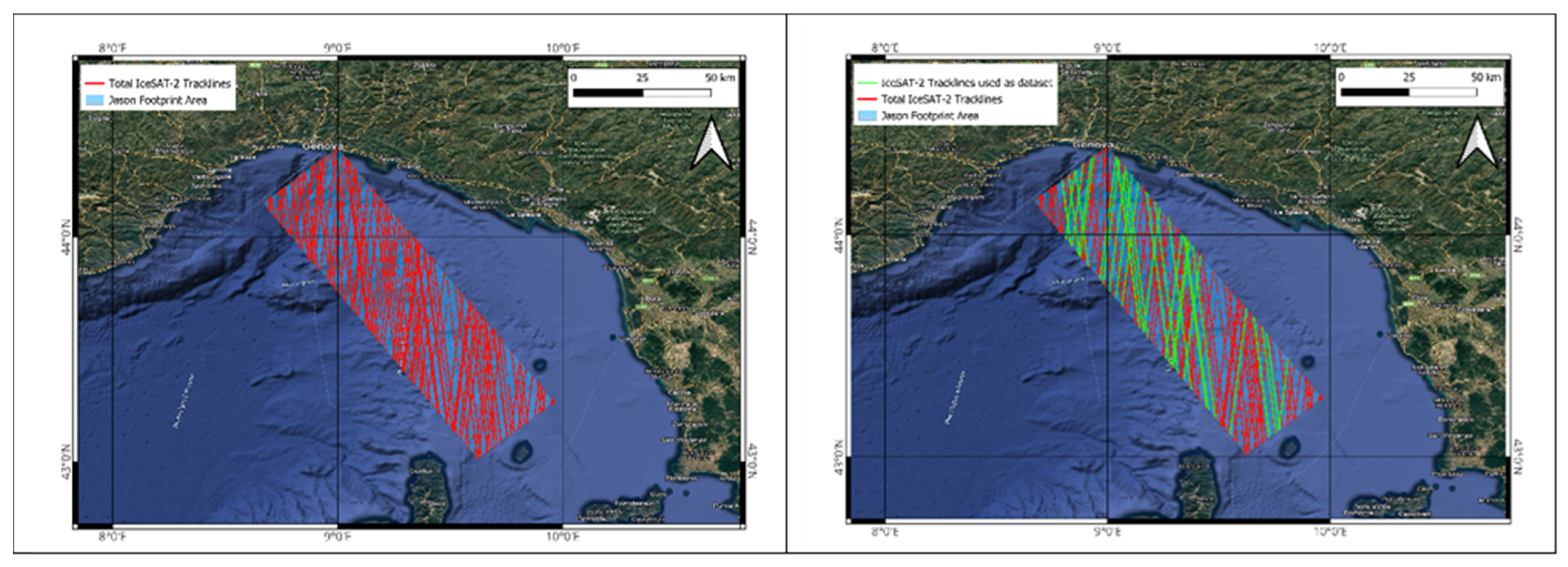
2.3. Satellite Altimetry Data

Radar altimetry used for this study is the satellite-based sea-level data processed by the X-TRACK system [40]. This product (called L2P) consists of along-track sea level anomaly (SLA) from all Topex/Jason-1/Jason-2/Jason-3 satellite cycles from March 1993 to April 2022. The X-TRACK product has recently been used in several oceanographic studies [41,42,43], and detailed descriptions of its processing evolution can be largely found in the literature [42,44]. The accuracy of the altimetric measurements has improved from 4.5 cm of the TOPEX/Poseidon to 2.5 cm of Jason3. Tidal corrections are computed by FES2012 [45], a global tidal model based on 93 harmonic components obtained by the analysis of the altimetry data. Dynamic Atmospheric Correction (DAC) includes the static inverted barometer correction at periods higher than 20 days, while MOG2D-G, a barotropic model [46] forced by atmospheric pressure and wind from ERA-Interim reanalysis data, is used to describe higher frequency ocean variability.
Track n.0044, which crosses the Tyrrhenian and Ligurian Seas from the south to the north, is repeated about every ten days, and data are about 6 km apart. The first considered point of the track is located at the latitude 43.112° N; 9.79° E (point n.236); the last, which is closest to the coast, is at 44.314° N; 8.81° E (point n.263), a total of 28 points for a total length of about 150 km.
As the XTRACK product does not cover the whole period of investigation, Sentinel-3B data along the ground track 099 were also used. Sentinel-3A is the first satellite to operate in Synthetic Aperture Radar (SAR) mode over the entire global ocean [47]. The new measurements are being validated around coasts in several worldwide regions, giving improved 3–4 cm accuracies that are as close as 2–3 km to the coast [48]. Unfortunately, no data were processed for either September or October 2023 passes. The two tracks do not exactly overlap. Sentinel 099 track deviates about 9° to the east with respect to Jason 44, and they cross at 43.6° N; 9.37° E. Sentinel-3 20 Hz-sampled data were analyzed from latitude 43.16° N to 44.3° N. Data corrected for tides and atmospheric effects are at a distance of 300 m. They were firstly smoothed with a 10-point moving average and then bin-averaged over 10 points, obtaining a spatial resolution of 3000 m and a total of 41 points.
ICESat-2 is a satellite launched on 15 September 2018 as part of NASA’s EOS program. The ICESat-2 mission was designed to assess changes in polar ice volume in order to establish a correlation and actively monitor sea level changes and ocean circulation. It follows a semi-polar orbit with an inclination of 92° at an altitude of about 500 km and a revisit time of 91 days. The satellite is equipped with a photon-counting LiDAR that emits 6 beams of light in the green band (532 nm) with a pulse repetition rate of 10 kHz, allowing it to estimate the ellipsoidal heights of objects hit by its emitted beam, reflecting photons back to the receiving sensor [49,50,51]. The along-track horizontal resolution is approximately 70 cm between consecutive measured points. As for accuracy, no official data are provided by the manufacturer, but some papers offer a vertical comparison between ICESat-2 measurements and tide gauges. In particular, [52] reports an average measured difference of 2.1 cm and a standard deviation of 11.1 cm. Although the system was primarily launched for ice monitoring, it also provides other elevation data, and for the purposes of this work, the focus was on the laser reflection on the sea surface.
The extraction of the ICESat-2 bathymetric signals was developed with Python 3.12.8 scripts in two phases: data automatic download and waterline detection [53]. All data from the launch of a satellite in October 2018 up to the latest available data during the analysis period for this work, October 2023, were downloaded. The area of interest used is the footprint of the JASON satellite: all available data were downloaded (Figure 3). For each satellite pass, only the central band with the ‘strong’ emission type was selected to use a single dataset for each pass. The selected data were processed and referenced to the EGM-2008 geoid and tide corrected; then, as suggested by [54], the water surface was identified as the median height within a moving window, in our case, composed of 51 points. From the totality of the data, only those that included a well-identified and complete water surface line were selected, excluding datasets with ‘noise’ or ‘spikes’. Thus, the dataset used was reduced from 187 total passes to 38.

2.4. ADCP Data

Surface current observations are very scarce in the region. Historical data from previous experiments [55] were recovered for this analysis. In particular, ADCP data collected in the area from 13 September 2003 to 24 May 2004 were recovered to allow the comparison between computed surface geostrophic currents from altimetry. The ADCP was mounted on a mooring line located at 43.79° N and 9.05° E at about 1000 m depth, close to the W1M3A Multidisciplinary Observatory [56] and to the altimetric track. The 300 kHz RDI ADCP was at 60 m below the sea surface in a looking-up configuration, set at 8 m bin size and 1 h sampling time, thus providing current measurements very close to the surface. For this analysis, data were daily averaged and smoothed with a 5-point centered moving window.

2.5. Dynamic Height and Geostrophic Currents Computation

Dynamic height was computed by integrating the specific volume over the upper 275 m of the water column, which is a common level to the majority of the available CTD profiles. This layer well includes the seasonal thermocline and most part of the mesoscale variability. Two stations (n.11 and n.12) were not considered as the sea bottom, which is below 250 m. To estimate the contribution of a deeper layer to the variation in surface dynamic height, a comparison was conducted for winter 2022 data using 850 m and 275 reference levels. The main difference (0.7 cm) between the 275 m reference level and 850 m is below the altimeter accuracy and was found at 44° N, but the general pattern is well preserved. The poor sensitivity of dynamic height gradients to the reference level [57,58] is a great advantage as this can limit the seawater column observations to the upper layer, reducing the time required to complete the measurements. Moreover, it makes the use of moving vessel profiling systems particularly appropriate for this kind of investigation [59].
Surface across-track components of the geostrophic currents from the altimetric measurements were computed by V = g dh/(f L), where dh is the difference of the elevation between each pair of points, L is the distance, f is the Coriolis parameter at the latitude between the two points, and g is the gravity.
The two points of the track close to the ADCP, namely points #249 and #253, located, respectively, at 43.69° N, 9.34° E and 43.87° N, 9.19° E, were chosen for this computation. The distance between them is 24 km, lower than the 50 km suggested by the theory for the geostrophic computation in the open oceans [60], but higher than the local Rossby radius, which is about 10 km [12]. During the period covered by the ADCP measurements, 26 satellite passes—from 389 to 414—were available, but 3 of them had no data. Data were smoothed with a 5-point moving average.

3. Results

3.1. TS Distribution and Dynamic Height

Temperature and salinity distribution along the transect well evidence the difference between the warmer and saltier Tyrrhenian waters and those of the Ligurian Sea. The inflow of Levantine Intermediate Water (LIW) entering from the Corsica Channel occupies the layer between 250 m and 500 m and can also be tracked in all the reported vertical sections describing the upper 300 m of the water column (Figure 4). At the upper interface of the LIW, some meanderings, particularly well-developed on the Winter 2022 map, appear. They are associated with the complex dynamic of this area, in particular with the presence of the Ligurian Anticyclone (LA), which occupies the southeast part of the Ligurian Sea [36,61], and the north–south frontal region separating the WCC from the ECC at about 9.2° E, which is crossed by the transect around 43.6° N. At the northern edge, another smooth surface temperature gradient identifies the front separating the near-coastal warmer and less salty waters from the open-sea circulation. During late summer, a saltier and warmer surface layer, resulting from the intense summer evaporation, characterizes the upper 30 m. During winter, the mixed layer is better evidenced by the temperature sections showing the vertical thermal structure almost uniform in the whole examined layer (0–300 m). Interannual differences can be mainly ascribed to the presence of the frontal region that is well-marked in winter 2024 but not in 2023. The temperature and salinity distribution confirm the well-known presence of eddies and mesoscale activity in the Ligurian Sea [12,13,37].
Summer and winter CTD-computed dynamic heights (Figure 5) are clearly separated by a bias of about 8 cm. This value is close to the steric level contribution of the observed seasonal variability of the mean sea level at the Genoa tidal station [62]. Despite this relevant seasonal difference, summer and winter surface topography along the examined tracks share some common patterns. The main pattern can be described by a general decrease from the southern part of the track with a minimum of about 44° N and an increase moving north to the coast, indicating the persistent large-scale cyclonic circulation of the Ligurian Sea. The difference in height from the southern part and the minimum can reach 7–8 cm with no relevant seasonal difference. Superimposed to this signal, the surface signature of different and less persistent features can be identified. In particular, the presence of the LA, whose center is located at about 43° N but has a strong variability in terms of shape and intensity, can be responsible for the differences evidenced in the southern part of dynamic heights. Winter 2022 data display some more variability, with two relative maxima at 43.7° N and 44° N. This situation is consistent with a second anticyclonic recirculation in the northern part, which is not uncommon during summer but not in winter.

3.2. Altimetry

3.2.1. Preliminary Data Check

Before the detailed analysis, the whole X-TRACK dataset underwent a preliminary evaluation. There are much missing or unreliable data close to the northern coast (points 260–263) until 2001, while the series is almost complete in the middle of the basin; only 13% of missing data were found in the time series of SLA at point 250. SLA at this point (Figure 6) has a well-pronounced annual cycle with high SLA in summer and minimum in winter. Maxima amplitude was reached in 2002, with a summer–winter difference of 30 cm. A six-month period of variability also results from spectral analysis and can be particularly well identified by two small relative maxima during 2007, 2015, 2016, and 2018.
DAC contribution to sea level variations is relevant as it spans a range from −20 cm to +10 cm. Spectral analysis evidences the main peak on the annual cycle, but for the rest, the spectrum is rather noisy, and the mesoscale atmospheric variability cannot be resolved due to the 10-day sampling period. Tidal and atmospheric correction time series over the period 2009–2016 in the point closest to the coast were previously checked against sea-level and atmospheric pressure data from the tidal station in Genoa [62]. The comparison provided satisfactory results, and the atmospheric corrections were mainly determined by the inverse barometric effect, but no other checks could be performed for the open sea. Tidal corrections along the analyzed track are almost uniform, with a maximum slope of 1 cm/150 km, which is consistent with the observations, such as the data from tidal stations of Centuri, close to Cape Corse, and those on Genoa.
Along-track variation in DAC displays a smooth increase in the sea level from the southern point to the coast during summer and a decrease during winter. Nevertheless, the majority of sea level variations over the track vary within the small range of less than 2 cm. This seems to underestimate the effects of several common meteorological and oceanographic situations characterizing the area. In particular, it poses some doubts about how the sea surface circulation is generated by the well-known cyclogenesis of the Ligurian Sea [15] or how the effect of mesoscale activity can be properly described. Differences of atmospheric pressure up to 6 mb between the open sea and the coast associated with specific meteorological events such as strong northern winds (Tramontana and Mistral) as well as downburst occurrences [63], are not uncommon in this area. Moreover, pressure differences higher than 2 mb between the W1M3A observatory and the port of Genoa are quite often observed [64].

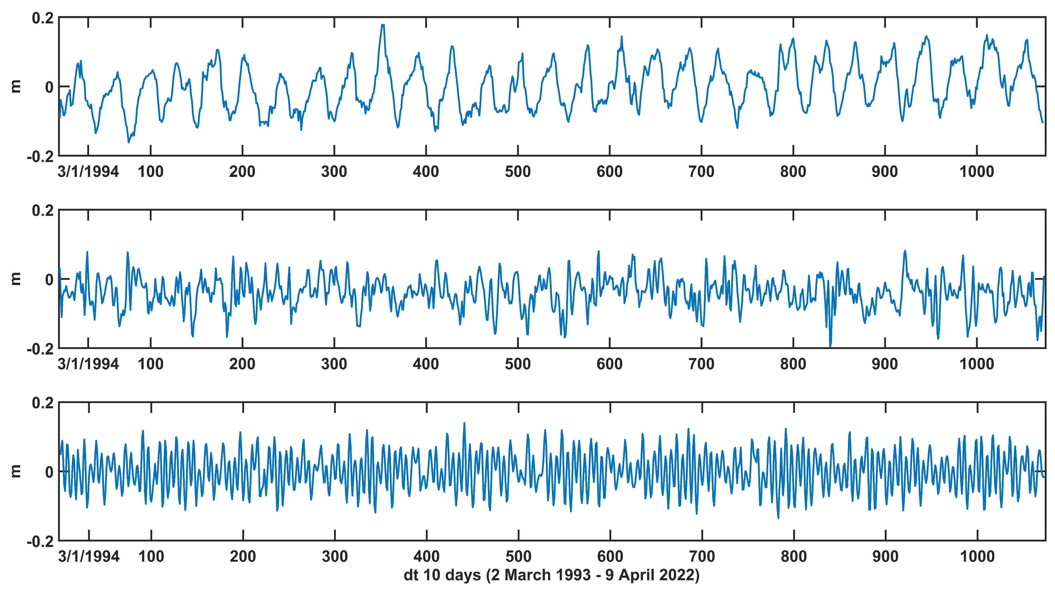
3.2.2. Jason and Sentinel Data

Altimetric data from 1994 to 2022 from X-TRACK products were grouped into monthly sub-sets, each of them being the average over 81–88 tracks. January, February, and March, as representative of the winter situation, and August, September, and October for the summer, were selected (Figure 7).
The two groups of altimeter profiles are separated by a bias that reaches a maximum of 16 cm between March and October at 43.7° N. This is consistent with the winter–summer steric level variation observed in the area. March is the period when the water column is quite uniform in temperature, with minimum values around 13.5 °C [55,65]. The maximum surface temperature in the Ligurian Sea is generally in late August, but the heat is stored along the water column until early October [66].
The range of variation along the examined track never exceeds 5 cm for all the profiles, but the standard deviation is quite high: 5.4 cm for the winter data and 5.8 cm for summer, without relevant spatial variations. Both winter and summer altimeter profiles are quite smoothed and flat—ranging within less than 1 cm—in the southern part up to about 43.8° N; then, a clear increase to the north occurs in winter, while during summer, it decreases. This is the main evident difference between the two situations.
While SLA profiles are in good agreement with the intensified cyclonic circulation of the Ligurian Sea during winter, the summer profiles seem to reflect the higher dynamic variability characterizing the eastern side of the Ligurian Sea. In particular, the role of the Ligurian Anticyclone, according to [36], can occupy the whole area from the Corsica Channel to the Italian coasts and seems responsible for coastal currents inversion and ECC modulation. The poor synopticity represents one of the main limits when comparing steric levels from CTD casts and sea level anomalies from satellite altimetry. The same satellite orbit is repeated every 10 or 30 days, while the opportunity for concurrent at-sea experiments occurred very seldom, and the in situ measurements required about two days. The satellite passes nearest to the CTD campaigns were selected from the dataset (Figure 8), but even a few days delay between the satellite pass and the oceanographic campaigns can be enough to allow the mesoscale activity to affect the signals [10]. A clear example is provided by the two altimetric profiles collected on 16 and 26 September 2017 in correspondence with the CTD campaign of 21–22 September 2017 along the same track.
SLA of 26 September agrees quite well with the CTD computed dynamic height, sharing the main shape characterized by a well-marked minimum at 43.9° N. Nevertheless, the situation is quite different if we consider the Jason pass on 16 September, which lags the same time interval from the campaign. The same occurs in winter 2022: the SLA profile of the Jason pass of 20 March 22 follows the pattern of the dynamic height, evidencing the two relative maxima at 43.7° N and 44° N missing the increasing trend to the northern coast, characterizing the winter profiles. Again, the Sentinel pass on 25 March is more similar to the ‘typical’ winter profiles than to the one taken five days before. On the contrary, the situation obtained from the campaign of 7/8 March 2024 is well represented by both the satellite data taken on 25 February and 23 March.

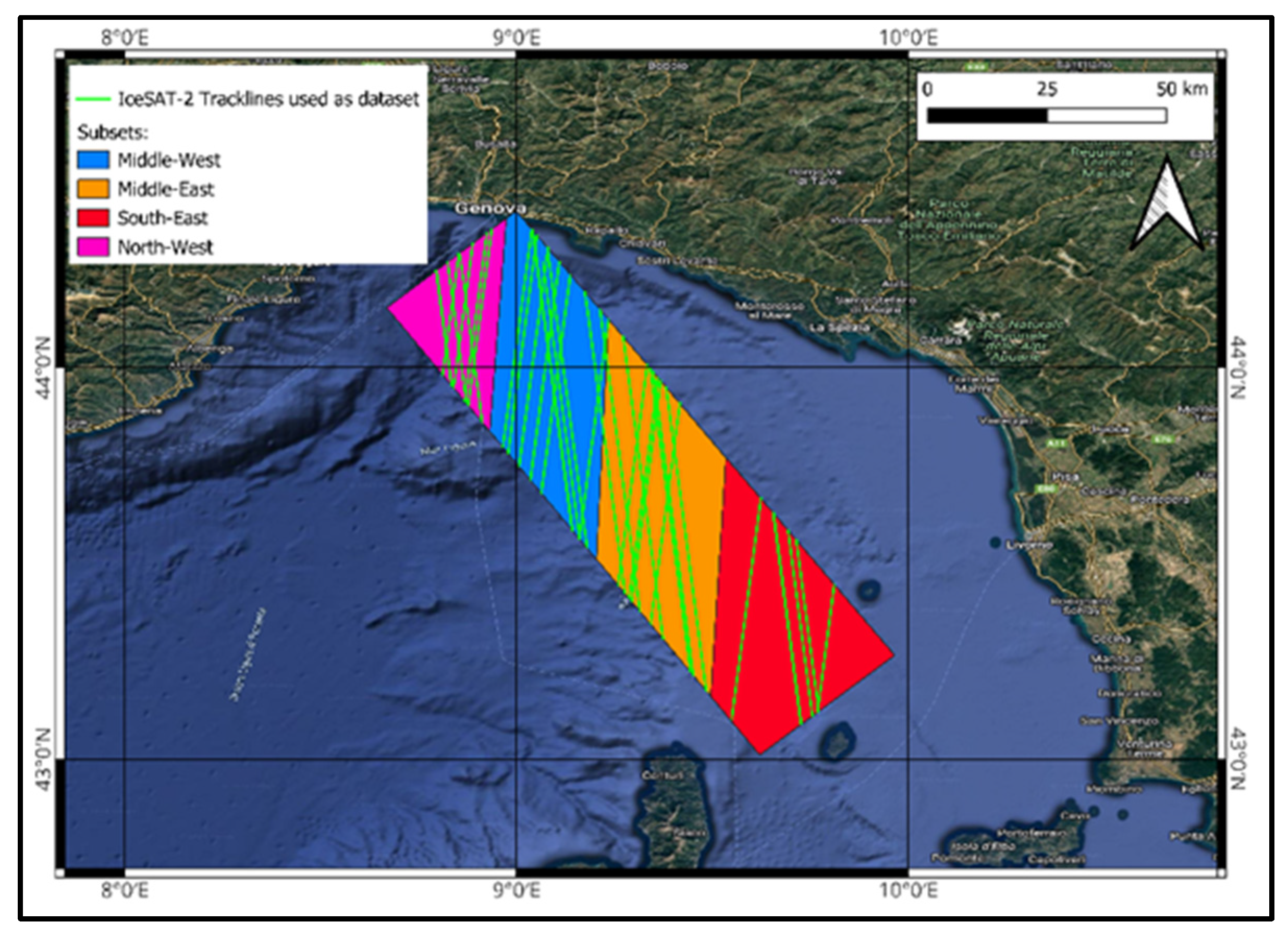
3.2.3. ICESat Altimetry

The different orbital characteristics of the JASON and ICESat-2 satellites make a direct comparison between the signals challenging, primarily because the intersection points between the orbits are too few, both spatially and temporally.
To perform a qualitative assessment, the area was divided into four more or less equivalent sub-areas, each with a similar number of orbital passes (Figure 9). Within these areas, a comparable number of satellite passes were included, specifically, northwest: 9 tracks; middle-west: 10 tracks; middle-east: 11 tracks; southeast: 8 tracks. For each of the sub-areas, the sea surface levels were plotted using four different colors according to the season: red for summer, yellow for autumn, blue for winter, and green for spring.
Figure 10 displays the plots of each subset: on the y-axis, we have the elevation (in meters) relative to the zero level of the EGM-2008 geoid, while on the x-axis, the latitude is represented in decimal degrees, increasing from left to right.
This type of data is not yet a routine analytical activity for assessing sea surface levels, but we can at least qualitatively evaluate certain behavioral patterns.
The northwest area and the southeast area, which are closer to the coast, show a fairly distinct sea level difference between the winter period (blue) and the summer period (red), with a relative elevation difference of several tens of centimeters.
On the other hand, the middle-west and middle-east areas, located in the more central part of the Ligurian Sea, have more random and noisy sea surface elevations, but at the same time, they show a more consistent and repeated surface morphology pattern over time. Specifically, the plot for the northwest subset reveals a well-defined, repeated pattern over time, with a sea level rise in the southern part, at the center of the Ligurian Sea, and a drop toward the north, in the coastal area.

3.2.4. Altimeter-Derived Geostrophic Currents and ADCP Observations

ADCP from fixed mooring represents another important observation platform for the assessment of derived satellite altimetry geostrophic circulation and surface in situ currents. The examined ADCP dataset depicts a surface circulation characterized by a prevailing northwestward direction (Figure 11). The available data in the upper 50 m show an almost barotropic flow; the near-surface current only slightly differs from the layers below. The average surface current over the whole period has a speed of 10.2 cm/s and direction 328°N (East −5.3 cm/s std 11.7; North 8.7 cm/s, std 11 cm/s). A frequent occurrence of inertial currents having a period of 17.3 is well evidenced by the time-frequency and spectral analysis (Figure 12). Inertial currents dominate the sub-daily variability, reaching amplitudes higher than the average speed. No tidal currents are detected due to the small tidal amplitude of the region.
The strong signal on inertial frequency also explains the poor correlation between the wind and the surface currents (complex correlation is only 0.35), which can also be inferred from the wind roses in Figure 11. Filtering the sub-daily variability by averaging over 24 h and smoothing with a five-span centered moving average only increases the correlation between wind and current to 0.49, indicating a minor role of the local wind with respect to the thermohaline forcing. The contribution of the wind on the surface currents of this dataset was also previously investigated [55] by means of Ekman models and EOF decomposition [67]. The second EOF mode resulted well correlated to the simulated Ekman currents, describing a prevailing southwest variability and evidencing the smaller contribution with respect to the total signal.
Significant variations seem mainly related to important mesoscale activity, with a time scale of about two weeks. This results in northeast deviations of the currents with respect to the regular and more intense northwestern movements. Spectral analysis on daily mean data of atmospheric pressure from the W1M3A observing system and currents can provide some indication about their relation, as both spectra have important peaks on 30, 16, and 12 days. Relevant seasonal patterns cannot be evidenced, but the time series spans over nine months, leaving most of the summer period far from this analysis.
The role of the atmospheric correction (DAC) was also investigated. Horizontal atmospheric pressure gradients over the sea have an important role in surface circulation through the inverse barometer effect, which can modify the sea surface by about 1 cm for each 1 mb of pressure variation. This is of particular importance in the Ligurian Sea, where deep and persisting low-pressure systems over the center of the basin are generated and are able to affect the circulation. The analysis of DAC and TIDE provided by the X-TRACK product over the 24 km track considered for the geostrophic current computation does not show significant spatial variability (rms between the two selected points is below 1 mm). As the computation is based on the relative slope between the two points, it was decided not to take them into consideration.
For the comparison with the computed geostrophic currents, only the cross-track component of surface ADCP data was considered. The mean value is close to zero (−0.3 mm/s), and the standard deviation is 9.5 cm/s. Cross-track currents range between −24.6 cm/s and 23.5 cm/s, with an average speed of 7.6 cm/s. To filter out inertial and other high-frequency fluctuations, daily mean data, smoothed with a five-span centered moving average, were used.
The comparison with the altimetric-derived geostrophic current (Figure 13) was first performed by considering the direct point-to-point difference as well as the ten-day averaged data, which fit with the time interval of satellite passes. Root mean square differences (RMSD) were 12.1 cm/s and 10.3 cm/s, respectively, in the same order as the standard deviation of the cross-track component (9.5 cm/s). Even if the direct measure of the wind-driven currents is not possible, a reliable assessment would require isolating the geostrophic component from the others. To eliminate the ageostrophic contribution—mainly ascribed to the wind—from the measured ADCP surface currents, the second EOF mode was subtracted from the signal. As the currents are strongly barotropic, another test was performed by analyzing the layer below the surface, namely at a depth between 8 m and 16 m, where the influence of the wind can be considered negligible. In the two cases, the RMSD only improved to 9.7 cm/s and 10.8 cm/s, respectively.

4. Discussion and Conclusions

The capability and potentiality of satellite altimetry to improve the knowledge of the Ligurian Sea surface circulation are assessed by means of the comparison of in situ observations. Differently from other satellite parameters such as temperature or salinity, the comparison of altimetry and in situ measurements can be only indirectly performed through derived quantities. The accuracy of a direct observation is defined and checked by the calibration of the instrument or by the analytical procedure, and the same cannot be obtained when a parameter is computed using a mathematical relation describing the physical process or by means of numerical models. If we add the different spatial-temporal sampling involved, we can easily understand how the obtained results, despite being useful and relevant, can be mainly qualitative. In this study, sea-level anomalies and the derived geostrophic surface currents were checked against dynamic heights computed from CTD casts along the track and surface currents time series measured by an ADCP mounted on a fixed mooring.
The main features of the seasonal circulation of the Ligurian Sea, as deduced by the average climatological surface topography observed by altimeters, enlighten the winter basin-scale cyclonic circulation characterizing the area. The climatological summer pattern is not straightforwardly interpreted as the few examined cases—both the CTD-derived surface topography and the SLA—do not follow the same climatological pattern. The variation in intensity, shape, and position of the LA, the occurrence of flow reversing in the northern part of the Corsica Channel [38], and the weakness of the cyclonic circulation contributes to the high interannual variability observed in the summer altimetric profiles.
Winter–summer bias between the SLA over summer and winter tracks agrees with the steric level changes related to the seasonal cycle of heat storage in the water column, thus representing a good indicator for climatic studies.
Track 044 follows quite closely the ferry route from Genoa to Palermo, which was chosen as a key route for Operational Oceanography programs and included repeated XBT measurements [36]. Vignudelli [68] first analyzed the SLA from altimetry and the dynamic height computed from the XBT along the route. The lack of concurrent salinity measurements—which would have reduced the errors on dynamic height computation—was compensated for by the huge amount of available observations over the same track. The RMSD between altimeter measurement and dynamic height for the Ligurian Sea was estimated in the small range of 2–4 cm along the whole track. The limited number of observations of this study does not allow a reliable estimation of RMSD, but the analyzed dynamic height computed from CTD cast and SLA from satellite altimetry have shown generally quite good similar patterns. Discrepancies can be ascribed to several factors, such as the lack of synopticity, low accuracy of altimeter measurements, and the presence of changing mesoscale [69]. The use of a barotropic model for the DAC estimation, even appropriate for large oceanic areas, could not take into consideration the high variability of the density distribution of the area due to the presence of different water masses as well as the effects of the complex bottom topography [70] and the coast.
ICESat data, although not specifically developed for the investigation of ocean topography and not yet an operational product, are able to identify persistent features and their variability. In the near future, they will represent an additional and important source of information, particularly because of their high spatial and temporal coverage.
Despite the test of different metrics to compare ADCP surface currents with the altimeter-derived geostrophic currents, the point-to-point difference did not provide enough good results as the RMSD was of the order of the standard deviation of the signal. There are several problems that hamper a reliable comparison between direct currents measurements and computed. Current meters measure the resulting movement generated by all forces acting in the region, both geostrophic and ageostrophic, so it is not possible to correctly isolate the geostrophic contribution from the ADCP profiles. Moreover, in this particular case, the main current direction was along the satellite track, while geostrophic computation only provides the cross-track component. When assessing these results, we cannot neglect that the accuracy of sea-level anomalies can be of the same order as the height difference between a couple of points used for the geostrophic computation. Nevertheless, the obtained results are comparable to those from similar experiments [71] involving long-term ADCP surface currents time series on the West Florida Shelf. Despite the experiment being planned to catch the along-coastal current, the wind-driven component was eliminated from the signal by means of numerical models, and the available time series was longer; no relevant improvements were evidenced.
This work confirms how the use of satellite altimeters can be of great support for the investigation of several oceanographic processes in the Ligurian Sea. As the geostrophic currents describe the main part of circulation at supra-daily periods and the circulation also in the upper thermocline is mainly barotropic, the use of an altimeter to derive the geostrophic part of the currents can strongly contribute to the description of the large-scale circulation in this region.
Even though sea surface topography is considered a surface observation, satellite measurements can also reveal relevant features that involve the water column, which cannot be easily detected by the sporadically available observations inside the water column. As an example, the variation in the steric level detected by the satellite altimetry strongly depends on the amount of heat stored in the water column. The analyzed time series of sea level anomaly indicates the highest summer maximum in 2002 (Figure 6), while, among the frequent heat waves affecting the Mediterranean region [72,73], the one that occurred in 2003 was remembered as one of the most devastating for the associated mass mortality [66,74]. This can shed new light on the approach of climatic studies, helping to better understand the complex mechanism related to ocean warming.
This study also adds important insights into assessing and possibly exploiting satellite altimetry in coastal oceanography studies. It represents an important case study to guide the technical and scientific evolution of altimetry toward its operational use within coastal observing systems [75].
During the last 15 years, the altimetry community has made a great effort to improve altimeter data in coastal seas and consequently develop customized products for exploitation. At present, the bibliography is rich in papers focusing on the improvement/development and much less on using the new/improved datasets in regional oceanography studies. As mentioned in the introduction, the aim of this paper is to valorize the combination of satellite observations and in situ measurements in studying the regional/coastal surface circulation. The Ligurian Sea is an important test bed. It includes all sectors related to ocean (e.g., shipping, seafood, energy generation) and land (e.g., ports, shipyards, tourism). There is a clear need for scientific evidence on which political decisions are made for a sustainable Ligurian Sea. The scientific results of this paper contribute to the extension of the capacity of the Copernicus Marine Service [76] in supporting applications (e.g., maritime safety, sustainable use of marine resources, healthy waters, marine hazard services, ocean climate services). For example, the recent launch of the Copernicus Coastal Thematic Hub is one example of the attention related to coastal seas.
Concerning the evolution of satellite radar altimetry, it is important to highlight that the European Space Agency is evaluating the potential of wide-swath altimetry for the EU Copernicus program. The main objective is to provide a much improved operational monitoring of the ocean mesoscale variability for the Copernicus Marine Service [77].
Monitoring and forecasting ocean circulation requires ocean observations for calibrating and validating models. Satellite altimetry is key to providing information about sea level and surface circulation variability. Today, we have several altimeter flying, and the temporal and spatial sampling is much improved. The advent of imaging altimetry (e.g., SWOT) will permit to densify the spatial coverage. Our scientific work highlights that in situ observations are also key to observing the ocean interior and making a full integration with satellite observations.

Author Contributions

Conceptualization and methodology, P.P., R.N. and S.V.; software, L.R. and R.N.; formal analysis and investigation, P.P., R.N. and L.R.; writing—original draft preparation, writing—review and editing, P.P., R.N., L.R. and S.V. All authors have read and agreed to the published version of the manuscript.

Funding

This research received no external funding.

Institutional Review Board Statement

Not applicable.

Informed Consent Statement

Not applicable.

Data Availability Statement

CTD data are collected by the “Istituto Idrografico della Marina” and can be shared under request.

Acknowledgments

Thanks to the Italian Navy Captains and personnel of the Research Vessels involved in all the mentioned campaigns. Thanks to CF Maurizio Demarte, Head of the IIM Geophysics and Oceanography Dept. for his support of this research.

Conflicts of Interest

The authors declare no conflicts of interest.

References

  1. Fu, L.L.; Le Traon, P.Y. Satellite altimetry and ocean dynamics. Comptes Rendus Geosci. 2006, 338, 1063–1076. [Google Scholar] [CrossRef]
  2. Srinivasan, M.; Tsontos, V. Satellite altimetry for ocean and coastal applications: A review. Remote Sens. 2023, 15, 3939. [Google Scholar] [CrossRef]
  3. Cipollini, P.; Vignudelli, S.; Lyard, F.; Roblou, L. 15 years of altimetry at various scales over the Mediterranean. In Remote Sensing of the European Seas; Springer: Dordrecht, Germany, 2008; pp. 295–306. [Google Scholar]
  4. Pascual, A.; Pujol, M.I.; Larnicol, G.; Le Traon, P.Y.; Rio, M.H. Mesoscale Mapping Capabilities of Multi-satellite Altimeter Missions: First Results with Real Data in the Mediterranean Sea. J. Mar. Syst. 2007, 65, 190–211. [Google Scholar] [CrossRef]
  5. Poulain, P.M.; Menna, M.; Mauri, E. Surface geostrophic circulation of the Mediterranean Sea derived from drifter and satellite altimeter data. J. Phys. Oceanog. 2012, 42, 973–990. [Google Scholar] [CrossRef]
  6. Rio, M.H.; Poulain, P.; Pascual, A.; Mauri, E.; Larnicol, G.; Santoleri, R.A. Mean Dynamic Topography of the Mediterranean Sea computed from altimetric data, in-situ measurements and a general circulation model. J. Mar. Syst. 2007, 65, 484–508. [Google Scholar] [CrossRef]
  7. Vignudelli, S.; Cipollini, P.; Astraldi, M.; Gasparini, G.P.; Manzella, G. Integrated use of altimeter and in situ data for understanding the water exchanges between the Tyrrhenian and Ligurian Seas. J. Geoph. Res. 2000, 105, 19649–19663. [Google Scholar] [CrossRef]
  8. Vignudelli, S.; Cipollini, P.; Reseghetti, F.; Fusco, G.; Gasparini, G.P.; Manzella, G.M.R. Comparison between XBT data and TOPEX/Poseidon satellite altimetry in the Ligurian-Tyrrhenian area. Ann. Geophys. 2003, 21, 123–135. [Google Scholar] [CrossRef]
  9. Bouffard, J.; Pascual, A.; Ruiz, S.; Faugère, Y.; Tintoré, J. Coastal and mesoscale dynamics characterization using altimetry and gliders: A case study in the Balearic Sea. J. Geophys. Res. 2010, 115, C10029. [Google Scholar] [CrossRef]
  10. Borrione, I.; Oddo, P.; Russo, A.; Coelho, E. Understanding altimetry signals in the Northeastern Ligurian sea using a multi-platform approach. Deep. Sea Res. Part I Oceanogr. Res. Pap. 2019, 145, 83–96. [Google Scholar] [CrossRef]
  11. Vietti, C.R.; Albertelli, G.; Aliani, S.; Bava, S.; Bavestrello, G.; Cecchi, L.B.; Bianchi, C.N.; Bozzo, E.; Capello, M.; Castellano, M.; et al. The Ligurian Sea: Present status, problems and perspective. Chem. Ecol. 2010, 26, 319–340. [Google Scholar] [CrossRef]
  12. Casella, E.; Molcard, A.; Provenzale, A. Mesoscale vortices in the Ligurian Sea and their effect on coastal upwelling processes. J. Mar. Sys. 2011, 88, 12–19. [Google Scholar] [CrossRef]
  13. Marullo, S.; Salusti, E.; Viola, A. Observations of a small-scale baroclinic eddy in the Ligurian Sea. Deep. Sea Res. Part A Oceanogr. Res. Pap. 1985, 32, 215–222. [Google Scholar] [CrossRef]
  14. Trigo, I.F.; Bigg, G.R.; Davies, T.D. Climatology of Cyclogenesis Mechanisms in the Mediterranean. Mon. Weather. Rev. 2002, 130, 549–569. [Google Scholar] [CrossRef]
  15. Buzzi, A.; Davolio, S.; Fantini, M. Cyclogenesis in the lee of the Alps: A review of theories. Bull. Atmos. Sci. Technol. 2020, 1, 433–457. [Google Scholar] [CrossRef]
  16. Burlando, M. The synoptic-scale surface wind climate regimes of the Mediterranean Sea according to the cluster analysis of ERA-40 wind fields Theor. Appl. Climatol. 2009, 96, 69–83. [Google Scholar] [CrossRef]
  17. Pensieri, S.; Bozzano, R.; Schiano, E. Comparison between QuikSCAT and buoy wind data in the Ligurian Sea. J. Mar. Syst. 2010, 81, 286–296. [Google Scholar] [CrossRef]
  18. Gaillard, P.; Ravazzola, P.; Kontolios, C.; Arrivet, L.; Athanassoulis, G.A.; Stefanakos, C.N.; Gerostathis, T.P.; Cavaleri, L.; Bertotti, L.; Sclavo, M.; et al. Wind and Wave Atlas of the Mediterranean Sea; Consiglio Nazionale delle Ricerche: Roma, Italia, 2006; Volume 2, 420p. [Google Scholar]
  19. Barbariol, F.; Davison, S.; Falcieri, F.M.; Ferretti, R.; Ricchi, A.; Sclavo, M.; Benetazzo, A. Wind Waves in the Mediterranean Sea: An ERA5 Reanalysis Wind-Based Climatology. Front. Mar. Sci. 2021, 8, 760614. [Google Scholar] [CrossRef]
  20. Corsini, S.; Franco, L.; Inghilesi, R.; Piscopia, R. Atlante delle onde nei mari italiani-Italian Wave Atlas. Agenzia Per La Prot. Dell’ambiente E Per I Serv. Tec. Univ. Rome 2006, 3, 152. [Google Scholar]
  21. Cutroneo, L.; Ferretti, G.; Barani, S.; Scafidi, D.; De Leo, F.; Besio, G.; Capello, M. Near Real-Time Monitoring of Significant Sea Wave Height through Microseism Recordings: Analysis of an Exceptional Sea Storm Event. J. Mar. Sci. Eng. 2021, 9, 319. [Google Scholar] [CrossRef]
  22. Istituto Idrografico della Marina. Tavole di Marea 2020, II 3133; IIM: Genova, Italy, 2019; p. 123. [Google Scholar]
  23. Wüst, G. On the vertical circulation of the Mediterranean Sea. J. Geoph. Res. 1961, 66, 3261–3271. [Google Scholar] [CrossRef]
  24. Gostan, J. Comparaison entre les conditions hydrologiques et climatiques observées dans le Golfe de Gênes pendant les hivers 1962–1963 et 1963–1964. Cah. Hydrograp. 1967, 19, 391–416. [Google Scholar]
  25. Prieur, L.; D’Ortenzio, F.; Taillandier, V.; Testor, P. Physical Oceanography of the Ligurian Sea. In The Mediterranean Sea in the Era of Global Change 1: 30 Years of Multidisciplinary Studies in the Ligurian Sea; Migol, C., Nival, P., Sciandra, A., Eds.; Wiley: Hoboken, NJ, USA, 2020; pp. 49–78. [Google Scholar] [CrossRef]
  26. Fedele, G.; Mauri, E.; Notarstefano, G.; Poulain, P.M. Characterization of the Atlantic Water and Levantine Intermediate Water in the Mediterranean Sea using 20 years of Argo data. Ocean. Sci. 2022, 18, 129–142. [Google Scholar] [CrossRef]
  27. Millot, C. Circulation in the Western Mediterranean Sea. J. Mar. Sys. 1999, 20, 423–444. [Google Scholar] [CrossRef]
  28. Sparnocchia, S.; Manzella, G.; La Violette, P.E. The interannual and seasonal variability of MAW and LIW core properties in the Western Mediterranean Sea. In Seasonal and Interannual Variability of the Western Mediterranean Sea; La Violette, P.E., Ed.; Series Coastal and Estuarine Studies; American Geophysical Union: Washington, DC, USA, 1994; p. 177. Available online: https://agupubs.onlinelibrary.wiley.com/doi/abs/10.1029/CE046p0117 (accessed on 4 December 2024).
  29. Poulos, S.E. Water Masses of the Mediterranean Sea and Black Sea: An Overview. Water 2023, 15, 3194. [Google Scholar] [CrossRef]
  30. Schroeder, K.; Chiggiato, J.; Bryden, H.L.; Borghini, M.; Ben Ismail, S. Abrupt climate shift in the Western Mediterranean Sea. Sci. Rep. 2016, 6, 23009. [Google Scholar] [CrossRef]
  31. Astraldi, M.; Gasparini, G.P.; Manzella, G.M.R.; Hopkins, T.S. Temporal variability of currents in the eastern Ligurian Sea. J. Geophys. Res. 1990, 95, 1515. [Google Scholar] [CrossRef]
  32. Taupier-Letage, I.; Millot, C. General hydrodynamical features of the Ligurian Sea inferred from the DYOMEDE experiment. Oceanol. Acta 1986, 9, 119–131. [Google Scholar]
  33. Sammari, C.; Millot, C.; Prieur, L. Aspects of the seasonal and mesoscale variabilities of the Northern current in the western Mediterranean Sea inferred from the PROLIG-2 and PROS-6experiments. Deep.-Sea Res 1995, 142, 893–917. [Google Scholar] [CrossRef]
  34. Schroeder, K.; Haza, A.C.; Griffa, A.; Ozgokmen, T.M.; Poulain, M.P.; Gerin, R.; Peggion, G.; Rixen, M. Relative dispersion in the Liguro-Provençal basin from sub-mesoscale to mesoscale. Deep Sea Res. Part I Oceanogr. Res. Pap. 2011, 58, 209–228. [Google Scholar] [CrossRef]
  35. Astraldi, M.; Gasparini, G.P. The seasonal characteristics of the circulation in the north Mediterranean basin and their relationship with the atmospheric-climatic conditions. J. Geophys. Res. 1992, 97, 9531–9540. [Google Scholar] [CrossRef]
  36. Ciuffardi, T.; Napolitano, E.; Iacono, R.; Reseghetti, F.; Raiteri, G.; Bordone, A. Analysis of surface circulation structures along a frequently repeated XBT transect crossing the Ligurian and Tyrrhenian Seas. Ocean. Dynam. 2016, 66, 767–783. [Google Scholar] [CrossRef]
  37. Poulain, P.M.; Mauri, E.; Gerin, R.; Chiggiato, J.; Schroeder, K.; Griffa, A.; Borghini, M.; Zambianchi, E.; Falco, P.; Testor, P. On the dynamics in the southeastern Ligurian Sea in summer 2010. Cont. Shelf Res. 2020, 196, 104083. [Google Scholar] [CrossRef]
  38. Sciascia, R.; Magaldi, M.G.; Vetrano, A. Current reversal and associated variability within the Corsica Channel: The 2004 case study. Deep. Sea Res. Part I 2019, 144, 39–51. [Google Scholar] [CrossRef]
  39. Ravaioli, M.; Bergami, C.; Riminucci, F.; Langone, L.; Cardin, V.; Di Sarra, A.; Crise, A. The RITMARE Italian Fixed-Point Observatory Network (IFON) for marine environmental monitoring: A case study. J. Oper. Oceanog. 2016, 9 (Suppl. S1), s202–s214. [Google Scholar] [CrossRef]
  40. Birol, F.; Fuller, N.; Lyard, F.; Cancet, M.; Niño, F.; Delebecque, C.; Fleury, S.; Toublanc, F.; Melet, A.; Saraceno, M.; et al. Coastal applications from nadir altimetry: Example of the X-TRACK regional products. Adv. Space Res. 2017, 59, 936–953. [Google Scholar] [CrossRef]
  41. Escudier, R.; Renault, L.; Pascual, A.; Brasseur, P.; Chelton, D.; Beuvier, J. Eddy properties in the Western Mediterranean Sea from satellite altimetry and a numerical simulation. J. Geoph. Res. Ocean. 2001, 121, 3990–4006. [Google Scholar] [CrossRef]
  42. Birol, F.; Delebecque, C. Using high sampling rate (10/20 Hz) altimeter data for the observation of coastal surface currents: A case study over the northwestern Mediterranean Sea. J. Mar. Sys. 2014, 129, 318–333. [Google Scholar] [CrossRef]
  43. Jebri, F.; Birol, F.; Zakardjian, B.; Bouffard, J.; Sammari, C. Exploiting coastal altimetry to improve the surface circulation scheme over the central Mediterranean Sea. J. Geophy. Res. Ocean. 2016, 121, 4888–4909. [Google Scholar] [CrossRef]
  44. Roblou, L.; Lamouroux, J.; Bouffard, J.; Lyard, F.; Le Hénaff, M.; Lombard, A.; Marsaleix, P.; De Mey, P.; Birol, F. Post-processing altimeter data towards coastal applications and integration into coastal models. In Coastal Altimetry; Springer: Berlin/Heidelberg, Germany, 2011; pp. 217–224. [Google Scholar]
  45. Carrère, L.; Lyard, F.; Cancet, M.; Guillot, A.; Roblou, L. FES2012: A new global tidal model taking advantage of nearly twenty years of altimetry. In Proceeding of the 20 Years of Progress in Radar Altimetry Symposium, Venice, Italy, 24–29 September 2012. [Google Scholar]
  46. Carrère, L.; Faugère, Y.; Ablain, M. Major improvement of altimetry sea level estimations using pressure derived corrections based on ERA-interim atmospheric reanalysis. Ocean. Sci. 2016, 12, 825–842. [Google Scholar] [CrossRef]
  47. Donlon, C.; Berruti, B.; Buongiorno, A.; Ferreira, M.H.; Féménias, P.; Frerick, J.; Goryl, P.; Klein, U.; Laur, H.; Mavrocordatos, C.; et al. The Global Monitoring for Environment and Security (GMES) Sentinel-3 missio. Remote Sens. Environ. 2012, 120, 37–57. [Google Scholar] [CrossRef]
  48. Benveniste, J.; Cazenave, A.; Vignudelli, S.; Fenoglio-Marc, L.; Shah, R.; Almar, R.; Andersen, O.; Birol, F.; Bonnefond, P.; Bouffard, J.; et al. Requirements for a coastal hazards observing system. Frontiers in Mar. Sci. 2019, 6, 348. [Google Scholar] [CrossRef]
  49. Bagnardi, M.; Kurtz, N.T.; Petty, A.A.; Kwok, R. Sea Surface Height Anomalies of the Arctic Ocean from ICESat-2: A First Examination and Comparisons with CryoSat-2. Geophys. Res. Lett. 2021, 48, 93155. [Google Scholar] [CrossRef]
  50. Neumann, T.A.; Martino, A.J.; Markus, T.; Bae, S.; Bock, M.R.; Brenner, A.C.; Brunt, K.M.; Cavanaugh, J.; Fernandes, S.T.; Hancock, D.W.; et al. The Ice, Cloud, and Land Elevation Satellite—2 mission: A global geolocated photon product derived from the Advanced Topographic Laser Altimeter System. Remote Sens. Environ. 2019, 233, 111325. [Google Scholar] [CrossRef]
  51. Morison, J.H.; Hancock, D.; Dickinson, S.; Robbins, J.; Roberts, L.; Kwok, R.; Palm, S.P.; Smith, B.; Jasinski, M.F. ; The ICESat-2 Science Team. ATLAS/ICESat-2 L3A Ocean Surface Height, Version 4; National Snow and Ice Data Center: Boulder, CO, USA, 2021. [Google Scholar]
  52. Tomíc, M.; Andersen, B. ICESat-2 for Coastal MSS Determination—Evaluation in the Norwegian Coastal Zone. Remote Sens. 2023, 15, 3974. [Google Scholar] [CrossRef]
  53. Bernardis, M.; Nardini, R.; Apicella, L.; Demarte, M.; Guideri, M.; Federici, B.; Quarati, A.; De Martino, M. Use of ICEsat-2 and Sentinel-2 Open Data for the Derivation of Bathymetry in Shallow Waters: Case Studies in Sardinia and in the Venice Lagoon. Remote Sens. 2023, 15, 2944. [Google Scholar] [CrossRef]
  54. Ranndal, H.; Christiansen, P.S.; Kliving, P.; Andersen, O.B.; Nielsen, K. Evaluation of a Statistical Approach for Extracting Shallow Water Bathymetry Signals from ICESat-2 ATL03 Photon Data. Remote Sens. 2021, 13, 3548. [Google Scholar] [CrossRef]
  55. Picco, P.; Cappelletti, A.; Sparnocchia, S.; Schiano, M.E.; Pensieri, S.; Bozzano, R. Upper layer current variability in the Central Ligurian Sea. Ocean. Sci. 2010, 6, 825–836. [Google Scholar] [CrossRef]
  56. Bozzano, R.; Pensieri, S.; Pensieri, L.; Cardin, V.; Brunetti, F.; Bensi, M.; Petihakis, G.; Margo Tsagaraki, T.; Ntoumas, M.; Podaras, D.; et al. The M3A Network of Open Ocean Observatories in the Mediterranean Sea. In Proceedings of the MTS/IEEE OCEANS 2013, Bergen, Norway, 10–13 June 2013; pp. 1–10. [Google Scholar]
  57. Rio, M.H.; Pascual, A.; Poulain, P.M.; Menna, M.; Barceló, B.; Tintoré, J. Computation of a new mean dynamic topography for the Mediterranean Sea from model output altimeter measurements and oceanographic in situ data. Ocean. Sci. 2014, 10, 731–744. [Google Scholar] [CrossRef]
  58. Ruiz, S.; Pascual, A.; Garau, B.; Pujol, I.; Tintoré, J. Vertical motion in the upper ocean from glider and altimetry data. Geophys. Res. Lett. 2009, 36, L14607. [Google Scholar] [CrossRef]
  59. Meloni, M.; Bouffard, J.; Doglioli, A.M.; Petrenko, A.A.; Valladeau, G. Toward science-oriented validations of coastal altimetry: Application to the Ligurian Sea. Remote Sens. Environ. 2019, 224, 275–288. [Google Scholar] [CrossRef]
  60. Pond, S.; Pickard, G.L. Introductory Dynamical Oceanography; Butterworth-Heinemann: Oxford, UK, 1983; 329p, ISBN 9780080570549. [Google Scholar] [CrossRef]
  61. Iacono, R.; Napolitano, E. Aspects of the summer circulation in the eastern Ligurian Sea. Deep.-Sea Res. 2020, 166, 103407. [Google Scholar] [CrossRef]
  62. Picco, P.; Vignudelli, S.; Repetti, L. A Comparison between Coastal Altimetry Data and Tidal Gauge Measurements in the Gulf of Genoa (NW Mediterranean Sea). J. Mar. Sci. Eng. 2020, 8, 862. [Google Scholar] [CrossRef]
  63. Flamant, C. Alpine lee cyclogenesis influence on air-sea heat exchanges and marine atmospheric boundary layer thermodynamics over the western Mediterranean during a Tramontane/Mistral event. J. Geoph. Res. 2003, 108, 8057. [Google Scholar] [CrossRef]
  64. Picco, P.; Schiano, M.E.; Incardone, S.; Repetti, L.; Demarte, M.; Pensieri, S.; Bozzano, R. Detection and Characterization of Meteo-tsunamis in the Gulf of Genoa. J. Mar. Sci. Eng. 2019, 7, 275. [Google Scholar] [CrossRef]
  65. Kovačević, V.; Gačić, M.; Fusco, G.; Cardin, V. Temporal evolution of thermal structures and winter heat content change from VOS-XBT data in the central Mediterranean Sea. Ann. Geophys. 2003, 21, 63–73. [Google Scholar] [CrossRef]
  66. Sparnocchia, S.; Schiano, M.E.; Picco, P.; Bozzano, R.; Cappelletti, A. The anomalous warming of summer 2003 in the surface layer of the Central Ligurian Sea (Western Mediterranean). Ann. Geophys. 2003, 24, 443–452. [Google Scholar] [CrossRef]
  67. Thomson, R.; Emery, W.J. Data Analysis Methods in Physical Oceanography; Elsevier: Amsterdan, The Netherlands, 2014; p. 716. [Google Scholar]
  68. Vignudelli, S.; Cipollini, P.; Roblou, L.; Lyard, F.; Gasparini, G.P.; Manzella, G.; Astraldi, M. Improved satellite altimetry in coastal systems: Case study of the Corsica Channel (Mediterranean Sea). Geophys. Res. Lett. 2005, 32, L07608. [Google Scholar] [CrossRef]
  69. Miao, M.; Zhang, Z.; Qiu, B.; Liu, Z.; Zhang, X.; Zhou, C.; Guan, S.; Huang, X.; Zhao, W.; Tian, J.; et al. On contributions of multiscale dynamic processes to the steric height in the northeastern South China Sea as revealed by moored observations. Geoph. Res. Lett. 2021, 48, e2021GL093829. [Google Scholar] [CrossRef]
  70. Sarkisyan, A.S. Forty years of JEBAR—The finding of the joint effect of baroclinicity and bottom relief for the modeling of ocean climatic characteristics. Izv. Atmos. Ocean. Phys. 2006, 42, 534–554. [Google Scholar] [CrossRef]
  71. Liu, Y.; Weisberg, R.H.; Vignudelli, S.; Roblou, L.; Merz, C.R. Comparison of the X-TRACK altimetry estimated currents with moored ADCP and HF radar observations on the West Florida Shelf. Ad. Space Res. 2012, 50, 1085–1098. [Google Scholar] [CrossRef]
  72. Martınez, J.; Leonelli, F.E.; Garcıa-Ladona, E.; Garrabou, J.; Kersting, D.K.; Bensoussan, N.; Pisano, A. Evolution of marine heatwaves in warming seas: The Mediterranean Sea case study. Front. Mar. Sci. 2023, 10, 1193164. [Google Scholar] [CrossRef]
  73. Garrabou, J.; Gómez-Gras, D.; Medrano, A.; Cerrano, C.; Ponti, M.; Schlegel, R.; Bensoussan, N.; Turicchia, E.; Sini, M.; Gerovasileiou, V.; et al. Marine heatwaves drive recurrent mass mortalities in the Mediterranean Sea. Glob. Change Biol. 2022, 28, 5708–5725. [Google Scholar] [CrossRef] [PubMed]
  74. Garrabou, J.; Coma, R.; Bensoussan, N.; Bally, M.; Chevaldonne, P.; Cigliano, M.; Diaz, D.; Harmelin, J.-G.; Gambi, M.C.; Kersting, D.K.; et al. Mass mortality in Northwestern Mediterranean rocky benthic communities: Effects of the 2003 heat wave. Glob. Change Biol. 2008, 15, 1090–1103. [Google Scholar] [CrossRef]
  75. Laignel, B.; Vignudelli, S.; Almar, R.; Becker, M.; Bentamy, A.; Benveniste, J.; Birol, F.; Frappart, F.; Idier, D.; Salameh, E.; et al. Observation of the coastal areas, estuaries and deltas from space. Surv. Geoph. 2023, 44, 1309–1356. [Google Scholar] [CrossRef]
  76. Le Traon, P.Y.; Reppucci, A.; Alvarez Fanjul, E.; Aouf, L.; Behrens, A.; Belmonte, M.; Bentamy, A.; Bertino, L.; Brando, V.E.; Zacharioudaki, A. From observation to information and users: The Copernicus Marine Service perspective. Front. Mar. Sci. 2019, 6, 234. [Google Scholar] [CrossRef]
  77. Bonaduce, A.; Benkiran, M.; Remy, E.; Le Traon, P.Y.; Garric, G. Contribution of future wide-swath altimetry missions to ocean analysis and forecasting. Ocean. Sci. 2018, 14, 1405–1421. [Google Scholar] [CrossRef]
Figure 1. Upper left: the Mediterranean Sea with the Ligurian Sea enlightened in red. Lower left: main pattern of circulation in the Ligurian Sea. WCC—Western Corsica Current; ECC—Eastern Corsica Current; LPC—Ligurian-Provenҫal Current; LA—Ligurian Anticyclone. Right: The area of the investigation: Ligurian Sea—Western Mediterranean with high resolution bathymetry in meters. The light blue line is the track n.044 of Jason, and the dots indicate the position of CTD casts. The green line is the track n.099 of Sentinel-3. The blue dot indicates the position of the W1M3A observing system and the mooring; the yellow star is the IIM tidal station of Genoa.
Jmse 12 02281 g001
Figure 2. Distribution of hourly averaged wind speed and direction data collected by the W1M3A in the period July 2006–June 2007 [17].
Jmse 12 02281 g002
Figure 3. Left: a total dataset of ICESat-2 track lines: 187 red track lines; right: track lines used as a dataset: 38 green track lines over the red ones.
Jmse 12 02281 g003
Figure 4. OceanDataView maps of temperature and salinity from CTD profiles collected along Jason 044 tracks during the IIM oceanographic campaigns. Win—winter; Sum—summer. Precise dates are in Table 1.
Jmse 12 02281 g004aJmse 12 02281 g004b
Figure 5. Dynamic height computed from CTD casts along the track; reference depth is 280 m. S is Summer; W is Winter (see Table 1 for the corresponding dates).
Jmse 12 02281 g005
Figure 6. From the top: time series of SLA, DAC, TIDE at point 250 (43.73° N; 9.30° E) along track #044. Plotted data are smoothed with a 5-point moving average.
Jmse 12 02281 g006
Figure 7. Monthly mean SLA profiles from the X-TRACK dataset over the period 1993–2022.
Jmse 12 02281 g007
Figure 8. The pattern of SLA along the tracks Jason044 (upper) and Sentinel 099 (lower). For a better comparison, they are all referred to as their minimum values.
Jmse 12 02281 g008
Figure 9. Sub-areas used for the qualitative analysis of the datasets.
Jmse 12 02281 g009
Figure 10. Elevation (in meters) relative to the zero level of the EGM2008 geoid. From the top: northwest area, middle-west area, middle-east area, southeast area, as defined in Figure 9. Colors indicate the season: green for spring, red for summer, yellow for autumn, blue for winter.
Jmse 12 02281 g010
Figure 11. Wind roses of hourly data of wind from W1M3A (left) and ADCP surface currents (right) during the period 13 September 2003–8 March 2004. Wind direction indicates the provenience of the wind while surface current direction indicates the direction of the movements, so the versus of the two plots is the opposite. The wind statistics, lacking the summer period, differ from the annual one reported in Figure 2.
Jmse 12 02281 g011
Figure 12. Surface layer currents rotary spectrum (left) and spectrogram (right) : upper clockwise, lower anticlockwise. In both cases, a 240 h window length and 24 h time lag were used for a total of 246 samples.
Jmse 12 02281 g012
Figure 13. Time series of daily mean values of cross-track component of ADCP surface currents: in the layers 0–8 m (blu line) and 8–16 m (pink line), first EOF mode decomposition describing the surface geostrophic part of the signal (black); cross-track component of altimetry-computed geostrophic currents (red point).
Jmse 12 02281 g013
Table 1. CTD campaigns along J 044 Track and available satellite data. AR ITS Aretusa, AL R/V Alliance, LE R/V Leonardo. Ja Jason, Se Sentinel, * no data.
YearDateVesselMeasurementsLatitude ° N
Min–Max
Max DepthSatellite PassSatellite
201721–22/9ARCTD-IDR42.25–44.28Bottom16/9; 26/9Ja
202221–22/3ALCTD-SBE43.14–44.281500 m20/3; 25/3Ja
20232–3/2LECTD-IDR43.39–43.751100 m12/2Se
20235–6/10ALCTD-SBE43.28–44.28300 m16/9; 13/10Se *
20247–8/3ALCTD-SBE43.14–44.281500 m25/2; 23/3Se
Disclaimer/Publisher’s Note: The statements, opinions and data contained in all publications are solely those of the individual author(s) and contributor(s) and not of MDPI and/or the editor(s). MDPI and/or the editor(s) disclaim responsibility for any injury to people or property resulting from any ideas, methods, instructions or products referred to in the content.

