Acoustic Propagation and Transmission Loss Analysis in Shallow Water of Northern Arabian Sea

Abstract

This study investigates acoustic propagation and transmission loss in shallow water at an unexplored site in the northern Arabian Sea near the Pakistan coastline using a normal mode theoretical framework. Sound propagation in shallow water with range-independent bathymetry was analyzed using a customized Kraken C program to compute eigenvalues and eigenfunctions. The sound speed profile and clay silt sediment samples of the northern Arabian Sea, which characterize the water column and ocean bottom, respectively, were determined. Coherent and incoherent transmission losses for frequencies ranging from 50 to 500 Hz were calculated across different ranges and depths. Results indicate significant intensity fluctuations with increasing range, leading to higher transmission loss. Low frequencies (50–225 Hz) exhibit more significant transmission loss, while higher frequencies (230–500 Hz) show reduced loss. Transmission loss is higher for receivers at 19 m depth compared to those at shallower depths (8 m and 12 m) because the receivers are positioned near the layer of bottom sediments. Factors such as source and receiver depth, sediment properties, bottom roughness, and sound frequency significantly influence transmission loss. The novel dataset for the region supports the assessment of sonar performance, underwater communication, navigation, and marine life exploration.

1. Introduction

The acoustic characteristics of the ocean exhibit significant complexity and dynamic nature. The propagation of the acoustic signal is affected by various elements of the underwater medium, including depth, temperature, salinity, location, time of day, and season. However, these medium properties fluctuate unpredictably based on the shallow and deep-water divisions of the ocean [1]. Moreover, in shallow marine environments, geo-acoustic factors, including seabed structure, sound velocities, densities, and sound speed attenuations in seabed layers, substantially influence the properties of acoustic wave propagation [2].

According to [3], acoustic transmission at low frequencies in shallow water takes place inside the water column and also involves the sub-bottom. Shallow water propagation strongly interacts with acoustic energy and the ocean floor. Their frequency determines the interaction between signals and usually occurs up to a few wavelengths below the surface, depending on the signal’s intensity. The shallowness is determined by the ratio of the water column depth to the acoustic wavelength. Shallow water waves occur when the wavelength is significantly larger than the water depth. Mode theory is a practical, valid tool for the interpretation of shallow water propagation at low frequencies, which can be expressed as dimensionless parameters $“kh”$. The symbol “k” represents the horizontal wave number, whereas “h” represents the sea depth [4].

Acoustic propagation in the ocean is inherently difficult due to the presence of many inhomogeneities and variations [5]. Sound propagation in seawater is complicated due to the intricate interactions between the bottom and surface, which provide additional challenges during shallow water propagation [6]. This type of propagation occurs when each ray emitted from the source is reflected at the bottom. The wave equation helps describe how sound travels in the ocean. It considers the factors and boundary conditions that characterize the ocean environment. Several diverse approximations and numerical methods have been devised. Various models exist for describing acoustic propagation in the ocean, such as the spectral or fast field program (FFP), ray theory, parabolic equation models, multipath expansion approach, and normal mode theory [7]. Kexin et al. [8] have described an emerging methodology in shallow water acoustics that integrates scientific expertise in acoustic propagation with advanced machine learning algorithms to accurately predict frequency-dependent transmission loss and optimize sound propagation strategies in complex underwater environments. This approach tackles the task of precisely simulating sound propagation in intricate ocean settings despite having limited information about the environment and limited acoustic data. These strategies suit distinct applications and exhibit varying computational complexity and accuracy levels. Normal mode theory is commonly employed to address the issue of acoustic propagation in a stratified material. Hence, significant efforts in propagation modeling commenced with the research conducted by Pekeris [9], who formulated and utilized the normal mode theory to study the transmission of sound waves in a layered medium within shallow oceanic settings. The Pekeris model and its extensions are helpful in understanding sound propagation in the water, mainly when normal modes and coupling to the seafloor are considered. This endeavor was undertaken by [10] with the assistance of the SACLANTCEN propagation model. An updated edition of Kraken [11], published in collaboration with SACLANT, explores both range-dependent and independent approaches.

The most recent models for underwater acoustic propagation, noise, reverberation, and sonar performance have been developed using normal modes [12]. Underwater acoustics has extensively utilized normal mode methodologies. Scientists are continuously improving methods for solving the modal problem, and the innovative finite difference scheme has great potential in this area [13]. Apart from variations in temperature and salinity, sonar system performance is also affected by sea surface and bottom interactions in shallow water regions. These influences can be in the form of sound scattering, refraction, and attenuation [14]. The research on the impact of bottom sound speed on acoustic propagation in surface sound and negative gradient sound channels has already been published [15]. Furthermore, as a sound wave propagates across water, it experiences a reduction in its intensity. The phenomenon described is known as absorption loss, leading to a propagation loss that is proportionate to the distance traveled. The absorption loss strongly influences ocean bottom properties, and bottom attenuation also increases with the frequency [16]. The compressional wave velocity is the sea-bottom parameter that significantly influences acoustic propagation, as compressional wave (P-wave) velocity is very sensitive to changes in water content that are very near saturation. This effect becomes significant when the concentration is close to or at its maximum. The P-wave velocity grows from 98.9% to 99.96% when the saturation value rises, according to [17]. The presence of sediment layers in shallow water significantly influences the transmission of acoustic waves. The intensity is strongly affected by a shear wave as the mode’s order increases, and the penetration into the seafloor increases as well. The impact of sediment layers on sound transmission increases with higher penetration into the seafloor [18]. As the mode order increases, the penetration into the seafloor grows. It signifies a rise in frequency, resulting in more penetration into the bottom and a reduction in transmission loss. The enhanced penetration and reduced transmission loss associated with higher-order modes and frequencies result mainly from shorter wavelengths, facilitating deeper absorption into the bottom. In addition, Noufal et al. [19] studied acoustic propagation in shallow waters using a normal mode approach and indicated that higher-order waves propagate at steeper angles and penetrate the bottom.

Meyer et al. [20] investigated underwater sound transmission in shallow water situations with a sedimentary bottom, explicitly focusing on short-range scenarios. The geometrical characteristics, specifically source immersion, receiver immersion, and the distance between the source and receiver, significantly affect the transmission loss outcomes. The uncertainties in the speed of sound in water significantly affect the results. Consequently, this work examines the underwater sound transmission in shallow water environments of the Arabian Sea. The influence of source and receiver depths on transmission loss was also assessed. The velocity of sound was measured in the Arabian Sea to eliminate ambiguities associated with sound speed in water.

Shallow water propagation in ocean acoustics is effectively characterized by normal mode propagation [21]. Sanjana et al. [22] studied environmental factors in coastal waters that affect sound propagation. The environment is considered a shallow water waveguide with a clayey bottom, and the calculated TL for different frequencies over range and depth showed that the loss with respect to the range is more for low frequencies and decreases with an increase in frequency. The same type of ocean waveguide with clayey silt bottom is studied in this work. The normal mode Kraken C program was used to perform the simulation results. This study contributes novel insights to the existing knowledge regarding sound transmission in this specific geographic region of the northern Arabian Sea. We employed a fundamental theory of the normal mode Kraken C program, which demonstrates enhanced accuracy for low-frequency and shallow water environments in acoustic propagation and transmission loss calculations. The Kraken C software (version 2017) exclusively generates an output file containing eigenvalues and eigenfunctions. A specialized ocean model and associated MATLAB R2022b code have been created to compute transmission loss based on varying frequencies, distances, source/receiver depths, and bottom roughness. The established code can be utilized for further analysis. This study aims to measure the transmission loss, specifically for dealing with problems related to shallow water across different frequencies ranging from 50 to 500 Hz. The study also seeks to investigate the influence of the ocean bottom on sound transmission in the Arabian Sea, particularly in shallow waters. The ocean bottom is typically surrounded by various types of sediments, which significantly influence sound transmission in the water column. The research is conducted in a previously unexplored area of the northern Arabian Sea, which involves the actual sound speed profile of shallow water and gathering sediment samples. The actual ocean model of the northern Arabian Sea was considered, in which water column features, sediment acoustic properties, and variable depths of the source, receiver, and bottom properties were incorporated. These properties are also essential requirements for highly effective modeling in shallow water. Subsequently, the Kraken C normal mode program and MATLAB code were developed accordingly to cater to all these environmental parameters. Ultimately, the various exemplary simulation outcomes, together with their analysis, are given. This study could serve as a valuable theoretical framework for practical applications, such as distant target recognition, geo-acoustic inversion using low-frequency underwater acoustic data, underwater communication, marine life exploration, and sonar performance evaluation.

This article outlines three important innovations to the research endeavor, which are summarized below:

• Provided novel data by quantifying environmental parameters, such as temperature, conductivity, water density, salinity, sound velocity, and depth using the conductivity temperature and depth (CTD) apparatus, enabling the determination of the sound speed profile in the northern Arabian Sea.
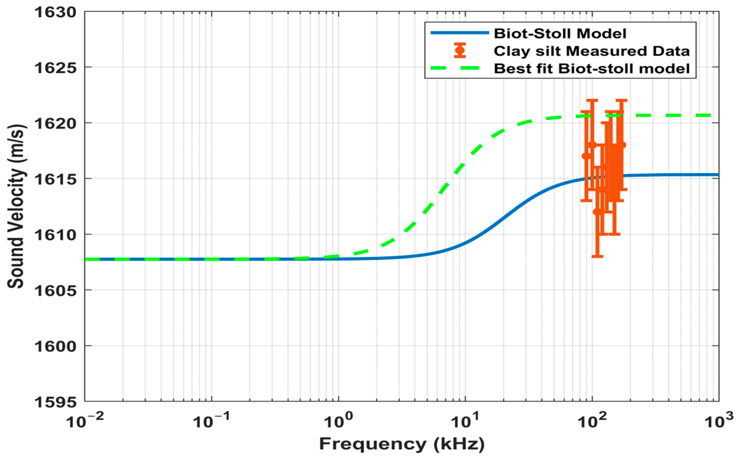
• Physical characteristics of sediment samples collected from the northern Arabian Sea were identified as clayey silt through categorization and sieve analysis. Additionally, bulk density, mean grain size, grain density, mass density, porosity, and acoustic properties, including sound speed and attenuation in sediment, were measured and analyzed from the laboratory experiments.
• Established the understanding of sound propagation characteristics within the low-frequency range of 50–500 Hz, highlighting the impact of the ocean floor on acoustic propagation, which is crucial for the advancement of underwater acoustic applications and the optimization of sonar system performance.

The paper is structured as follows: Section 2 covers the study region, sediment samples collection, and physical measurements. Section 3 explains the normal mode model and transmission loss calculations. Section 4 presents simulation results and analyzes sea bottom properties affecting sound propagation in shallow water. Finally, the study is concluded in Section 5.

2. Materials and Methods

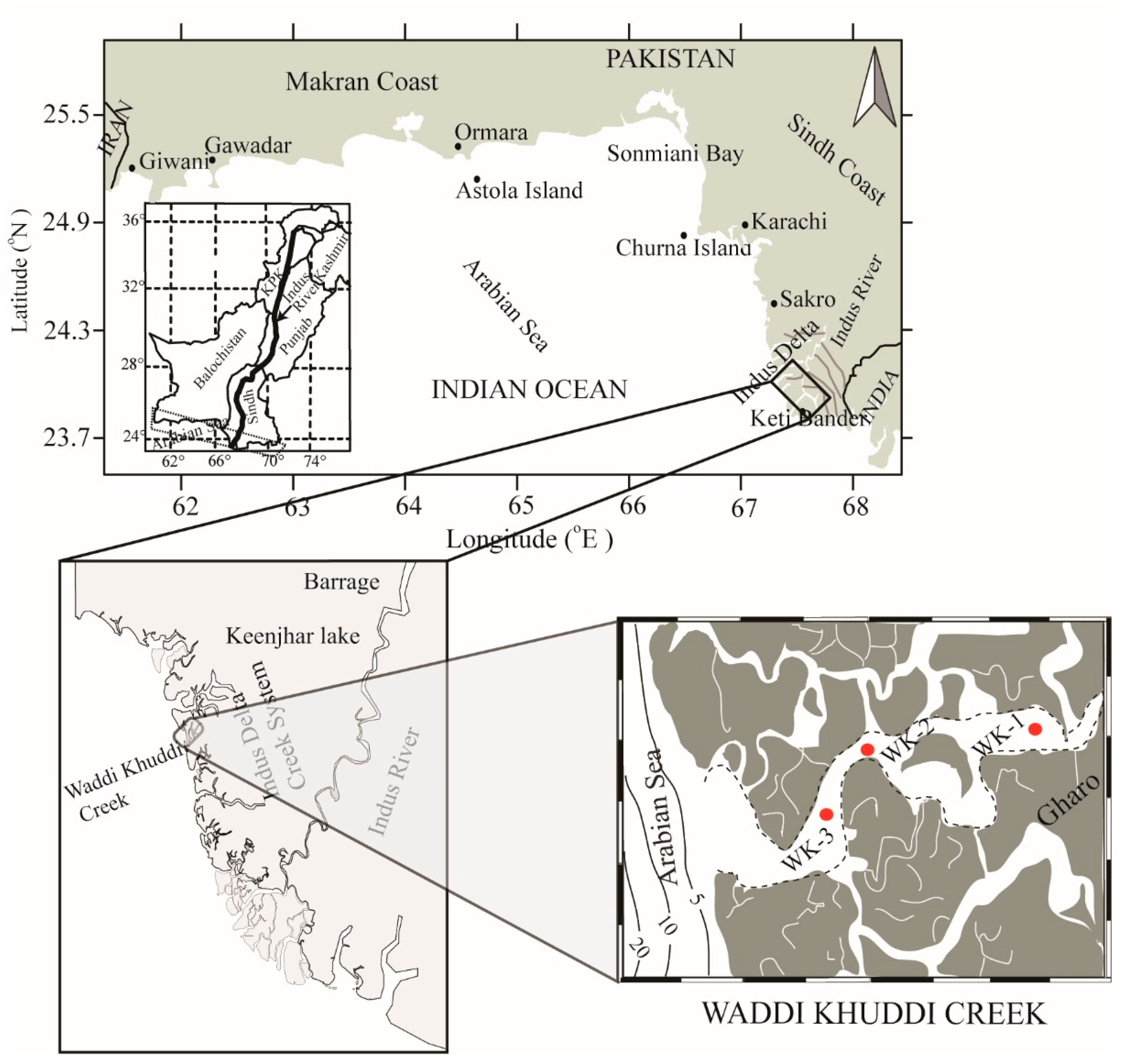
2.1. Study Site

The study site under investigation is situated in the Arabian Sea, adjacent to the Pakistan coastline. The Arabian Sea is positioned north of Pakistan and spans a coastline measuring 1001 km. The study location, known as Waddi Khudi Creek or Indus Delta coast near Karachi, had coordinates of 24.55° to 24.65° N latitude and 67.24° to 67.34° E longitude. A field survey in 2023 was conducted in the Waddi Khuddi Creek shallow water, which included three stations (WK-1, WK-2, and WK-3). Figure 1 depicts the geographic positioning of the study region. Using a sub-bottom profiler, the sediment sample was also obtained to calculate physical parameters from the Indus Delta coast site 19.0 m below the sea surface. The sea water’s temperature, salinity, and pH measurements at the sampling site near the bottom were recorded as 22.5 °C, 35.7 PSU, and 7.83, respectively. The sampling took place throughout February 2023, aligning with the spring season in Pakistan. Collecting genuine samples of marine sediments from the Arabian Sea is a significant challenge for precisely determining the exact physical characteristics and classification.

We have collected sediment samples and environmental data from three distinct locations in the shallow water of Arabian Sea, which are 2 km apart from each study site, for measurement and experimentation, as illustrated in Figure 1. The sampling process was repeated until the sample reached a weight of approximately 4 kg. The sediment volume should be at least 3 dm³ in order to ensure a reliable assessment of the acoustic properties and to satisfy the experimental requirement. This sediment sample was acquired through grab sampling. A Ponar sampler, which is composed of a pair of jaws that hold tightly to the seafloor upon contact, is frequently employed to acquire grab samples. We have conducted comprehensive acoustic measurements, including sound speed and attenuation of sediment samples, in our previous work, Shaikh et al. 2024 [23]. Those results are extended to low-frequency range measurement because the same sediment sample was utilized in this study. We have collected actual data from the Arabian Sea at a depth of 19 m and measured characteristics such as porosity, sediment density, seawater density, sound velocity in water, sound speed, and sediment attenuation. We have utilized a conductivity, temperature, and depth (CTD) apparatus to gather actual information from the undiscovered region of the Arabian Sea.

2.2. Physical Properties of Novel Sediment Sample

A sediment sample was collected from the Arabian Sea through a grab sampler, and its physical properties, such as mean grain diameter, sediment classification, and mass grain density, were determined using grain size analysis conducted in a laboratory at NIO, Pakistan. In order to measure the grain size, we took a sample of 50 g in weight and put it in a grain analyzer after drying to carry out sediment grain size classification based on [24]. A grain size analyzer can reveal the particle size distribution of a 50 g sample, which is essential for understanding the sediment’s depositional environment, permeability, dry bulk density, porosity, and other geological properties. The sediment is composed of clay, with a concentration of 86.6%, and silt, with a concentration of 13.4%. To determine the grain size, 13.4% of the sample passed through the sieve mesh having a diameter of 0.063 mm, and 86.6% passed through the sieve mesh having a diameter of 0.0039 mm. Subsequently, the grain diameter was calculated using Equation (1) as described in the literature [25].

$$d={\sum }_{i=1}^n{p}_i{d}_i, p_1+p_2+\dots +p_n=1$$

(1)

where $p_i$ denotes the frequency by weight for particles retained on the i th size class sieve whose diameter is $d_i$, n represents the number of particle-size classes in the sample, and d represents the mean grain diameter of the sample. The grade scale was proposed by [26] and modified by [27]. It is logarithmic, where each size class is twice as large as the next smaller class. Phi (φ) equals −log₂ (d), where d is the equivalent spherical diameter in millimeters. The U.S. standard wire meshes are used for sieving granules, sands, and coarse silt-size particles. In this paper, a sieve analyzer was used in the laboratory for accurate grain size measurement and classification of the sediment type as per the table mentioned in [28]. The characteristics of sediment, including particle size, density, and porosity, are critical elements affecting sound propagation in the ocean. All these parameters were measured in the laboratory with increased effort. The precise classification of sediments yields critical information for coastal engineering, environmental monitoring, and acoustic modeling, particularly in shallow waters. To determine the bulk density, we obtained a sediment sample with a volume of 100 cm³. This represents the total volume (solid grains, pore spaces, and water) prior to the drying of the sediment. Subsequently, the sediment may be heated in an oven at 105 °C for a minimum of 24 h. After drying, the samples were permitted to chill in a desiccator to avert moisture absorption from the atmosphere. Bulk density was determined by the ratio of the weight of dry sediment to the entire volume. Furthermore, to ascertain the sediment grain density, we filled the cup cylinder with deionized water to a specified capacity. Subsequently, we transferred the dried sediment sample of 100 cm³ to the cylinder in order to record the updated level and deducted it from the initial water level from the final water level to ascertain the sediment grain volume. Consequently, sediment grain density can be quantified by the ratio of the weight of dry sediment to the volume of the sediment grains. The physical parameters of the sediment sample were measured in the laboratory and are depicted in

Table 1. Measured physical parameters of sediment.

Parameters	Symbol	Unit	Measured Values
Silt concentration	-	%	13.4
Clay concentration	-	%	86.6
Mean grain diameter	d	mm	0.012
Mean grain size	Phi (φ)	-	6.4
Sediment grain density	${\rho }_g$	g/cm3	1.685
Sediment bulk density	${\rho }_b$	g/cm3	0.539
Porosity	$\beta$	-	0.680
Sediment density	${\rho }_s$	g/cm3	1.24

.

The northern Arabian Sea is one of the most productive maritime regions globally, attributable to many monsoon-related phenomena. The sediment sample from the northern Arabian Sea near the Pakistan coastline reveals several distinct characteristics that set it apart from other regions. The clayey silt sediment is predominantly composed of clay, with a very fine mean concentration of 86.6%, and silt with 13.4% has a very fine mean grain diameter of 0.012 mm. This results in a mean grain size of 6.4 Phi, indicating exceptionally fine particles. The sediment’s bulk density is notably low at 0.539 g/cm³, reflecting its high porosity of 0.680. This high porosity suggests a significant amount of void space within the sediment, which can absorb more water and reduce its overall density. The sediment grain density is 1.685 g/cm³, which is higher than the bulk density, while the overall sediment density is 1.24 g/cm³. These attributes imply that the sediment in this region is unusually fine and porous compared to sediments found in other areas. Such properties are likely to influence acoustic propagation in unique ways, potentially leading to increased scattering and attenuation of sound waves, which can affect underwater acoustic applications, such as sonar performance and communication. According to the sediment categorization, the sample was determined to be composed of clayey silt due to its mean grain diameter. Sediment grain density and bulk density were calculated in the laboratory by Equation (2) and Equation (3), respectively, as described in the literature [29].

$${\rho }_g={\displaystyle \frac{W_d}{V_g}}$$

(2)

$${\rho }_b={\displaystyle \frac{W_d}{V_t}}$$

(3)

where ${\rho }_g$ is the sediment grain density, ${\rho }_b$ is sediment bulk density, $W_d$ is the weight of dry sediment sample, $V_g$ is the volume of the sediment particles, and $V_t$ is the total sample volume. In addition, the sediment density was determined using the methodology outlined in the literature [30] and expressed by Equation (4). Furthermore, the porosity of the sediment can be determined by analyzing the correlation between its bulk density and sediment grain density, as indicated in Equation (5) proposed by [31].

$${\rho }_s=\beta \times {\rho }_w+(1-\beta )\times {\rho }_g$$

(4)

$$\beta =1-{\displaystyle \frac{{\rho }_b}{{\rho }_{\mathrm{g}}}}$$

(5)

where ${\rho }_s$ is the sediment density, ${\rho }_w$ is the water density, and $\beta$ is the porosity.

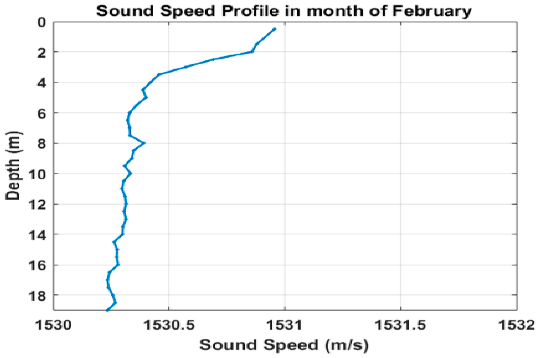
2.3. Sound Speed Profile

The sound speed profile (SSP) has a considerable impact on the way sound waves travel. SSPs play a vital role in underwater acoustics, oceanography, and marine research. The sound speed profiles included in this study for the northern Arabian Sea along the Pakistan coastline were acquired from multiple sources. The first source comprises the databases of surveys carried out by researchers and scientists affiliated with the National Institute of Oceanography (NIO), Pakistan. The present research utilizes CTD data obtained through a research vessel during the year 2023 in the Arabian Sea to compute the SSP. The researcher’s publications [19,32] collected temperature, salinity, and pressure data using a CTD device during a field investigation at Cochin estuary coastal waters and in the southeast Arabian Sea, respectively, for SSP computation. A CTD device was used to monitor environmental parameters, such as temperature, conductivity, water density, salinity, depth, and speed of sound. The World Ocean Atlas (www.nodc.noaa.gov, accessed on 24 February 2023) serves as the second data source, with monthly database reports and sound speed profile values for various geographical regions. The year-round data of sound speed profiles in the northern Arabian Sea near the coastline of Karachi, Pakistan, has been published by [33].

The sound speed profiles in the area often exhibit a very small gradient. This hinders the transmission of sound waves over long distances in shallow water. The current study was conducted in February 2023, specifically focusing on Karachi, Pakistan’s coastal environment, after the winter season’s end. Figure 2 and Figure 3 display the temperature and salinity data concerning depth collected using a CTD device in the research area. The speed of sound in the Arabian Sea is obtained from CTD data and confirmed by applying the formula described in Equation (6).

$$\begin{gathered} C=1448.96+4.591T-5.304\times {10}^{-2}{T}^2+2.374\times {10}^{-4}{T}^3+1.340\left(S-35\right)+1.630\times {10}^{-2}D \\ +1.675\times { 10}^{-7}{D}^2-1.025\times {10}^{-2}T\left(S-35\right)-7.139\times {10}^{-13}{TD}^3 \end{gathered}$$

(6)

The calculation of the speed of sound in seawater, denoted as C and measured in meters per second (m/s), may be determined using the Mackenzie equation [34]. Equation (6) is applicable within a temperature range of 2 to 30 °C, salinity of 25 to 40 parts per thousand, and depth of 0 to 8000 m. Let T denote the water temperature in degrees Celsius, D represents the depth in meters, and S represents the salinity in parts per thousand. Equation (6) above, which calculates the speed of sound in seawater based on temperature, salinity, and depth, is considered the most accurate and widely accepted among equations incorporating depth [35]. The sound speed profile for February 2023 is presented in Figure 4 after performing the sound speed computation. Temperature is the primary component that affects the calculation of sound speed. Consequently, the fluctuation of sound speed is primarily limited to the upper portion of the ocean depth.

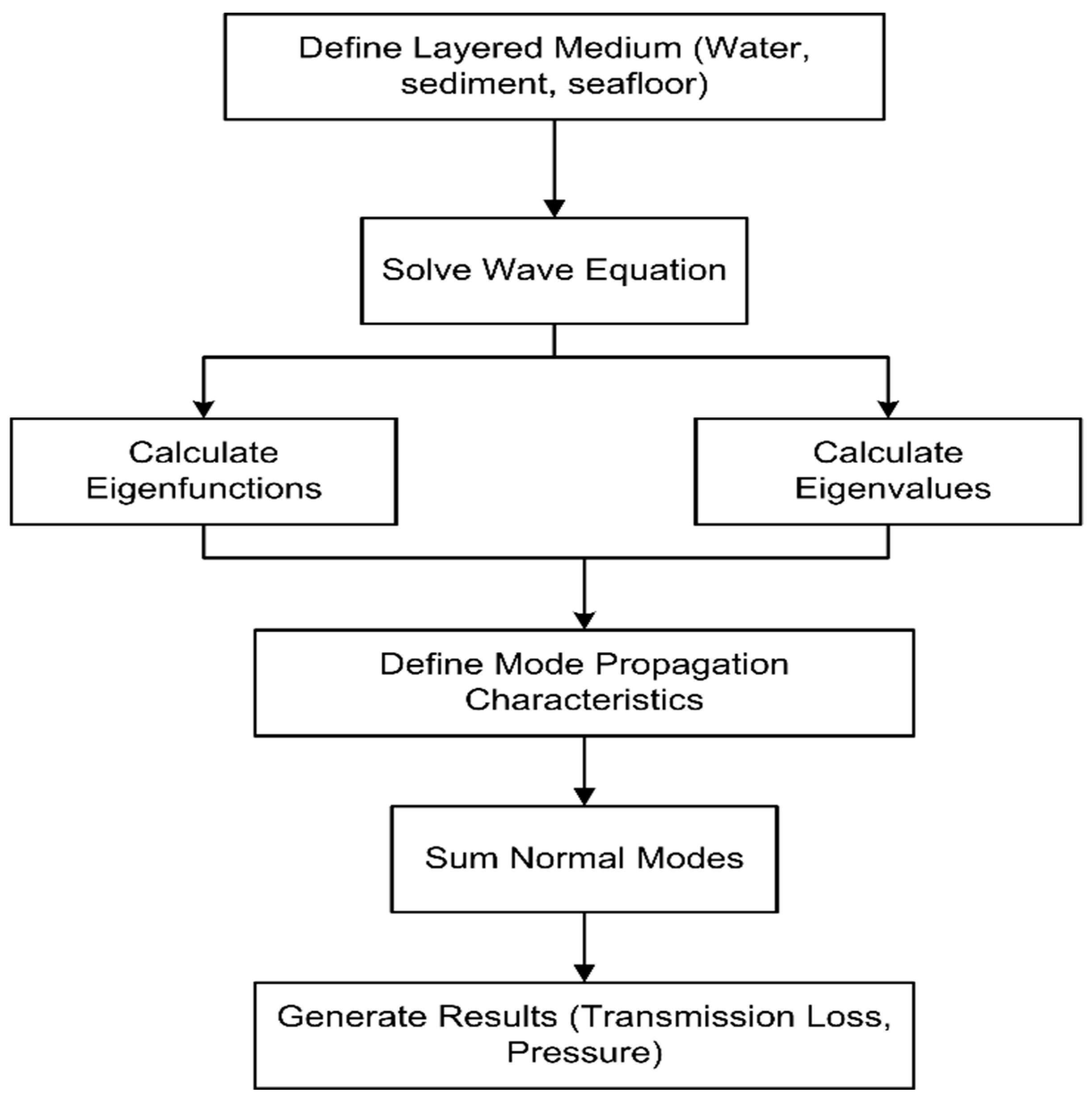
2.4. Normal Mode Program Kraken C

This article conducted numerical simulations using the Kraken C program. A two-layer seabed model comprising a fluid sediment layer and an underlying elastic half-space was proposed to clarify the interference pattern of sound waves observed in shallow water experiments. The experiment in [5], conducted at low frequency, was analyzed through the Kraken C program. Moreover, it was confirmed that the Kraken C program is superior to Kraken for the normal mode theory, as demonstrated by [20]. Thus, this research takes into account the same model as the actual sea environment and incorporates the parameters estimated in the northern Arabian Sea. This work serves as a comprehensive reference for the practical application of sonar systems, encompassing their performance and importance for researchers in the field of underwater acoustics.

3. Normal Mode Theoretical Framework

The mathematical model for the normal mode theoretical framework has been derived in accordance with the widely followed work by [16,36]. The two-dimensional Helmholtz equation [37,38,39] analyzes a point source in a horizontally stratified fluid medium, which has cylindrical symmetry about the z-axis, and its density and velocity only vary with depth, z. In this model, the acoustic pressure measured at the receiver can be expressed as a sum of the normal modes of the waveguide.

The conclusive equation of the pressure field is articulated in Equation (7):

$$p(r,z)={\displaystyle \frac{i}{4\rho (z_s)}}\sum _{m=1}^{\infty }{Z}_m(z_s)Z_m(z){H_0}^1(k_{rm}r)$$

(7)

This is the fundamental equation of normal mode theory used to determine the pressure field within the waveguide across various ocean environments, relying on the eigenvalues and eigenfunctions for its solution. Where r is the range, $z_s$ and z are the source and receiver depths, respectively, $\rho (z_s)$ is the density at the source depth, $m$ represents the number of modes, $Z_m$ is the normalized modal function of the mode or eigenfunction, and $k_{rm}$ is the horizontal wavenumber associated with mode or eigenvalues.

In this paper, normal mode theory is used as a mathematical approach employed to address issues related to wave propagation in complicated media, such as oceans, by breaking the problem into smaller, orthogonal modes. These modes denote the natural frequencies at which a system, such as the ocean or its layers, transmits waves. In underwater acoustics, normal modes are solutions to the wave equation that characterize the propagation of sound waves in a layered medium. The fundamental concept is that sound propagation may be expressed as a summation of “normal modes”, each associated with a unique propagation trajectory characterized by its specific speed and attenuation. The modes are determined by the parameters of the medium, including density, sound speed, and attenuation, and are influenced by the boundaries, such as the ocean surface, bottom, and sediment layers. Figure 5 illustrates the graphical depiction of normal mode theory as a block diagram.

Initially, the physical and acoustic characteristics of the environment, encompassing sound speed profile, density, water column depth, sediment, and seafloor features, are identified. These characteristics are critical parameters for calculating the wave equation and ascertaining the propagation of sound through the medium. The calculation of the wave equation yields eigenvalues and eigenfunctions that characterize the acoustic modes of the system. Consequently, mode propagation establishes the contribution of each mode to the overall sound transmission. The different modes are aggregated to form the entire sound field. The total number of modes is dependent upon the frequency, distance, and characteristics of the medium. The final stage entails utilizing the combined mode solutions to compute transmission loss (TL) and pressure fields. The same task is executed by the Kraken C program in this paper. The user provides all input data, including frequency, sound speed profile, density, water column depth, source depth, receiver depth, sediment, and seafloor characteristics in the “ENVFIL”. The output of a Kraken C program named “MODFIL”, includes computed eigenvalues and eigenfunctions. The MATLAB function will read the output file and compute the acoustic pressure field. The transmission loss is computed using MATLAB, generating multiple graphs according to the specifications.

Moreover, transmission loss (TL) encompasses both the loss due to geometrical spreading and the loss attributable to attenuation. Geometrical spreading refers to the reduction in acoustic energy as the sound wave propagates through space, while attenuation accounts for the gradual decrease in sound intensity as a result of energy absorption by the medium. TL plots are instrumental in visualizing how acoustic energy dissipates along the propagation path from the source, providing valuable insights into the effectiveness of sound transmission in various environmental conditions. Transmission loss, in decibels, can be calculated as the ratio between the acoustic intensity I (r, z) at a field point and the intensity $I_0$ measured at a 1 m distance from the source [40].

4. Simulation Results

The KRAKEN C normal mode program was utilized to conduct computer simulations to investigate the specific conditions of the Arabian Sea and the environmental factors that impact the sound field in this area. The sound source radiates a continuous signal at the frequencies, and the receiver receives the signal radiated by the source at a distance of 10 km. The simulation was conducted to calculate transmission loss across the range (10 km) and frequency (50–500 Hz) at different sources and receiver depths, which are as follows.

4.1. Shallow Water Propagation Modeling

The shallow water environment in the northern Arabian Sea near Pakistan’s coastline is characterized by using the measured sound speed profile and sediment data obtained at the study site. We assume that this shallow water environment can be accurately represented by the modal illustrated in Figure 6.

The ocean is modeled as taking a fluid layer of water 19 m deep. A sediment layer was obtained between the bottom half-space and the ocean. The sediment thickness in the northern Arabian Sea is unconsolidated and measured as a 1 m depth of sediment in this research area, which was identified after collecting the sample at the site and subjected to sieve examination. As shown in Figure 6, the scenario shows a soft layer of clayey silt sediment over a bottom basement, which is commonplace in most oceans. This area has a significant influence on the attenuation properties, especially because of fluid content, pressure, and rock types. In the northern Arabian Sea, specifically near the coast of Pakistan, the basement in this area typically consists of oceanic crust. Based on studies of this region, the compressional and shear wave velocities, attenuation, and other model parameters are estimated, as depicted in

Table 2. Geo-acoustic parameters of shallow water environment (temperature = 22.5 °C).

Parameters	Symbol	Unit	Range Values
Channel depth	H	m	19.0
Range	r	km	10
Speed of sound in water	$C_p$	m/s	See Figure 4
Water density	${\rho }_0$	$\mathrm{g}/{\mathrm{c}\mathrm{m}}^3$	1.025
Speed of sound in sediment	$C_p$	m/s	1607.75–1607.83
Sediment attenuation	$\alpha$	dB/km-Hz	0.02
P-wave speed in basement	$C_p$	m/s	4000
S-wave speed in basement	$C_s$	m/s	2000
Density in basement	${\rho }_{bas}$	$\mathrm{g}/{\mathrm{c}\mathrm{m}}^3$	1.9
P-wave attenuation in basement	${\alpha }_p$	dB/km-Hz	0.005
S-wave attenuation in basement	${\alpha }_s$	dB/km-Hz	0.01

. Moreover, ocean sediment is a kind of dispersive medium. Therefore, the velocity and attenuation in sediment change with frequency. These parameters were measured through experiments of sediment samples in the laboratory conducted by our previous work (Shaikh et al. 2024) [23] and extended the Biot Stoll model fitting curve with experimental data for the clayey silt sediment to lower frequencies (50–500 Hz). Results of the sound velocity and attenuation in sediments are illustrated in Figure 7 and Figure 8, respectively.

The shallow water environment under investigation is characterized by a channel depth of 19.0 m, with both the source and receiver positioned at a different depth to analyze the simulation results. The propagation range considered for this study is 10 km. In the water column, the speed of sound decreases with respect to depth from 1530.9 to 1530.2 m/s, and the water density is 1.025 g/cm³.

Figure 7 exhibits a speed of sound from 1607.75 to 1607.83 m/s within the frequency range of 50 to 500 Hz. Figure 8 exhibits sediment attenuation within the frequency range of 50 to 500 Hz. At a frequency of 50 Hz, the attenuation was approximately 0.001 dB/m, whereas at 500 Hz, it increased to 0.01 dB/m, demonstrating a linear correlation with frequency. However, in accordance with the requirements of the Kraken program, we must convert attenuation to dB/km-Hz. The sediment attenuation values at 50 Hz and 500 Hz were both 0.02 dB/km-Hz, as reported in Table 2. Consequently, in the low-frequency region of 50–500 Hz, it exhibits minor variation in dB/m. Consequently, we established the value as 0.02 dB/km-Hz for the clayey silt sediment within the frequency range of 50–500 Hz. Below the sediment, the basement consists of a more rigid material, assuming the parameter values as P-wave speed of 4000 m/s and attenuation of 0.005 dB/km-Hz, S-wave speed of 2000 m/s and attenuation of 0.01 dB/km-Hz, density of 1.9 g/cm³. These parameters provide a comprehensive overview of the acoustic properties of the shallow water environment, which are important for understanding sound propagation, attenuation, and overall acoustic properties in this region.

The sound propagation characteristics are considered to be a range-independent, dual-layer sea bottom model consisting of a clayey silt sediment layer and an underlying bottom half-space shallow ocean environment with a channel depth of 19 m. Initially, the task involves assessing the attenuation of signal strength, specifically at a frequency of 50 Hz, 200 Hz, and 500 Hz, respectively. The sound source radiates a continuous signal at these frequencies, and the receiver receives the signal radiated by the source at a distance of 10 km. The source of the current conditions in the northern Arabian Sea is located at a depth (Sd) of 12 m with different frequencies. The receiver (Rd) is 10 km away from the source and positioned at a depth of 12 m, as shown in Figure 6. The TL for different frequencies concerning the range is shown in Figure 9.

Since the environment consists of shallow water, cylindrical spreading is expected to be the main factor influencing the propagation. Figure 9 demonstrates that in cylindrical spreading, the intensity fluctuates severely as the range increases and subsequently increases the transmission loss. A point source is 12 m in the frequency band of (50–500 Hz), and receivers are located at different depths. The sound source radiates a continuous signal at these frequencies, and the receiver receives the signal radiated by the source at a distance of 2 km. Transmission loss for different receiver depths at the range of 2 km is shown in Figure 10.

The corresponding result illustrates the transmission loss (TL) of sound in an underwater environment with a clayey silt sediment bottom as a function of frequency (in Hz) and depth (in meters). The study is performed at a source depth (Sd) of 12 m and a range of 2.0 km from the source. Lower frequencies, ranging from 50 Hz to 225 Hz, undergo greater attenuation, particularly at specific depths, whereas higher frequencies, between 230 Hz and 500 Hz, often exhibit lower transmission loss. In the upper regions of the water column, transmission loss exhibits minimal change with depth, and the overall loss is mild (blue–green colors), signifying more uniform propagation. At greater depths, particularly near the sediment layer, there exist regions of elevated transmission loss (shown by yellow to red spots), especially at lower frequencies. This may result from heightened interactions with the clayey silt sediment layer, where sound waves experience greater attenuation at specific frequencies. Since a lossy bottom affects acoustic propagation at low frequencies, the 2 km range transmission loss demonstrates that the loss with respect to the range is highest at low frequencies and drops off sharply as the frequency increases. In addition, the research report conducted in coastal waters by [22] provides other evidence to validate this information.

4.2. Identification and Analysis of Environmental Parameters

Obtaining an accurate understanding of the environmental factors required for modeling acoustic propagation during experimental activities in the Arabian Sea is quite challenging. This section discusses the impact of wave frequencies and the effect of source and receiver depths. Next, we will evaluate the impact of bottom roughness on acoustic propagation. Then, a simulation is conducted to determine the incoherent transmission loss across a range of frequencies and receiver depths. As we know, the ocean is a complex and dynamic medium with varying temperature, salinity, pressure, and bottom properties. Incoherent transmission loss models predict these variations better by averaging out fast interference fluctuations. Consequently, we will examine the impact of each parameter individually.

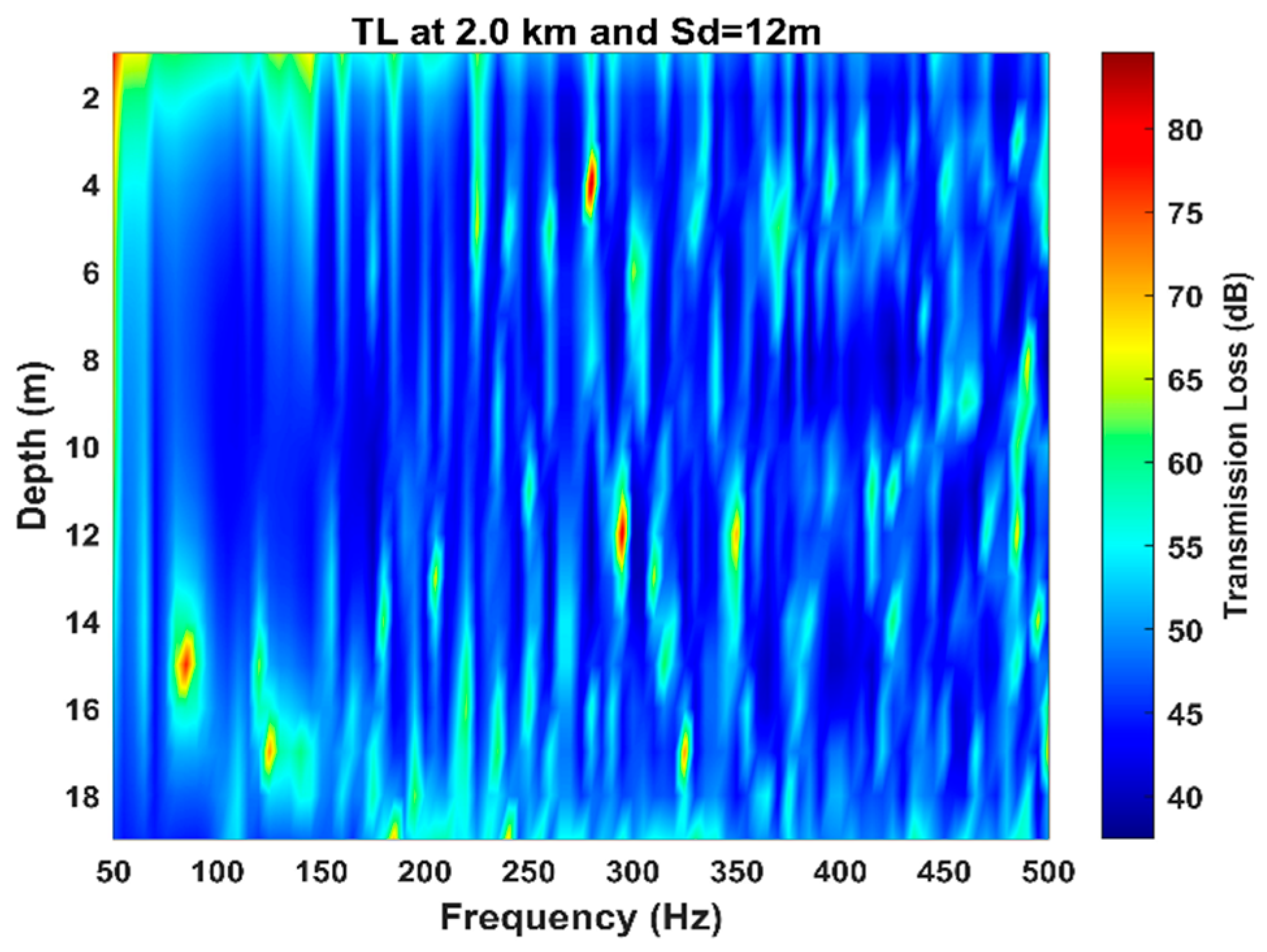
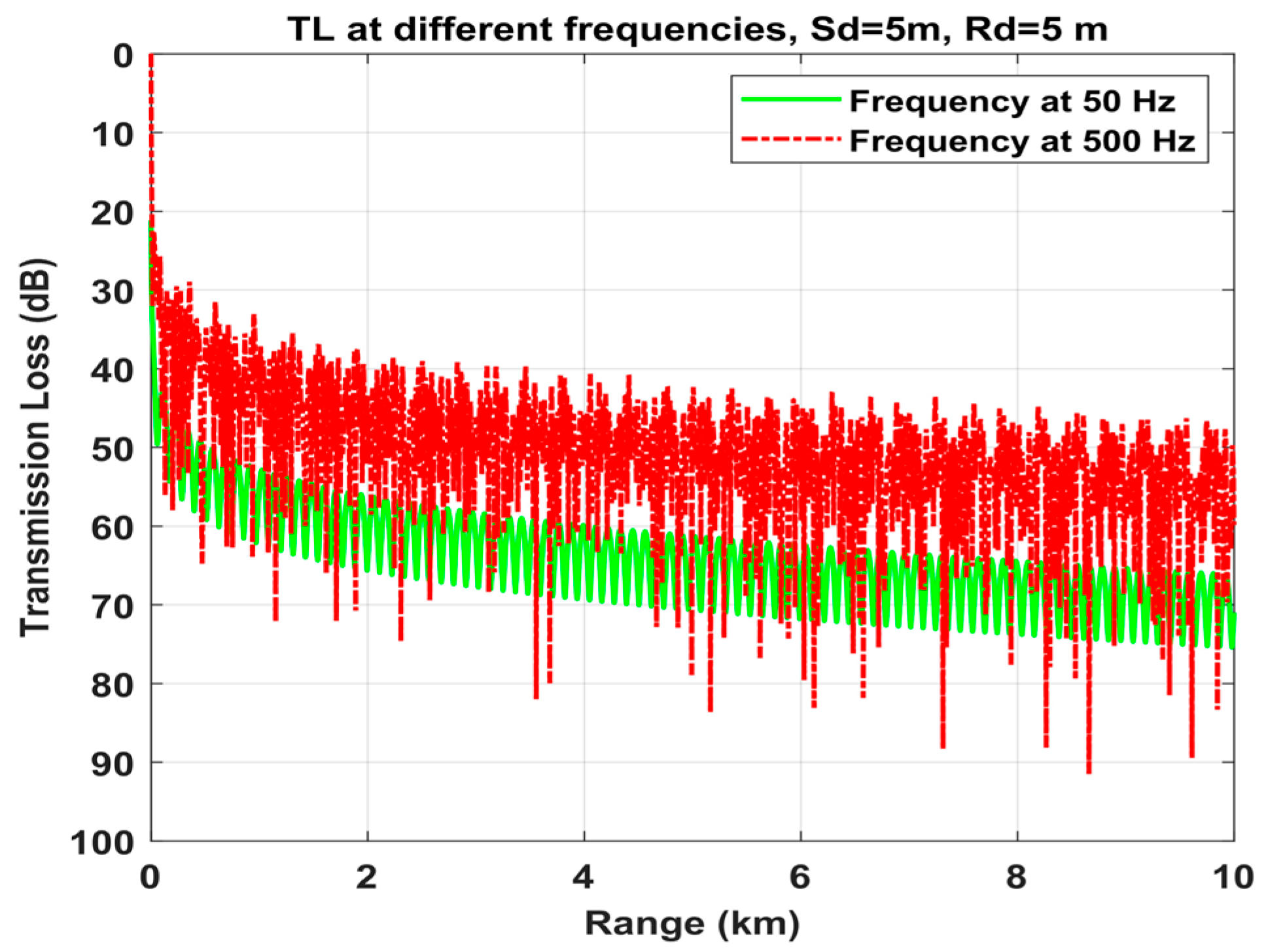
4.2.1. Wave Frequency Influence

The frequency of the source is crucial in the sound transmission process in shallow water. Hence, the source and receiver are stationary and positioned at a depth of 5 m, emitting distinct frequencies of 50 and 500 Hz, respectively. The distance between the receiver and the source is 10 km, and all other environmental factors are identical to those depicted in Figure 6. The sound source radiates a continuous signal at the given frequencies, and the receiver receives the signal radiated by the source at a distance of 10 km. Figure 11 illustrates the TL for two different frequencies, 50 Hz and 500 Hz, as sound travels through water over a range of up to 10 km. The solid green line indicates the TL at 50 Hz, and the dashed red line represents the TL at 500 Hz. The graph shows that TL fluctuates with range, and the fluctuations are more rapid for 500 Hz than for 50 Hz.

At both frequencies, transmission loss (TL) increases with distance, as anticipated, due to the dispersion of sound energy and the increased absorption and scattering at greater ranges. Moreover, at a low frequency of 50 Hz, only two propagation modes are observed, leading to higher transmission loss due to a lower absorption loss, and the overall TL is greater for 50 Hz at these distances. At a high frequency of 500 Hz, the number of propagation modes grows to nine, resulting in lower transmission loss due to higher absorption loss, as depicted in Figure 11. This could be due to several factors, including the specific environmental conditions of the water (temperature, salinity, depth) and bottom penetration, which can affect sound propagation differently at various frequencies. Furthermore, the number of normal modes diminishes as the wave frequency drops. Figure 12 illustrates the interference structure of the sound field and the transmission loss (TL) as a function of frequency (50–500 Hz) and range (0 km to 10 km) in shallow water, with the source depth (Sd) and receiver depth (Rd) both set at 5 m. The color scale on the right denotes the TL in dB, with blue signifying lower TL and red indicating higher TL, and the associated number of propagation modes is from two to nine, respectively. The red and yellow lines in Figure 12 highlight that frequencies around 50 to 100 Hz exhibit high transmission loss, suggesting their limited effectiveness for long-distance sound propagation in the underwater environment compared to other frequencies. Transmission loss varies with respect to the different frequencies in this region of the Arabian Sea. This information is crucial for applications, such as underwater communication, navigation, and acoustic sensing, where selecting the appropriate frequency can significantly impact performance.

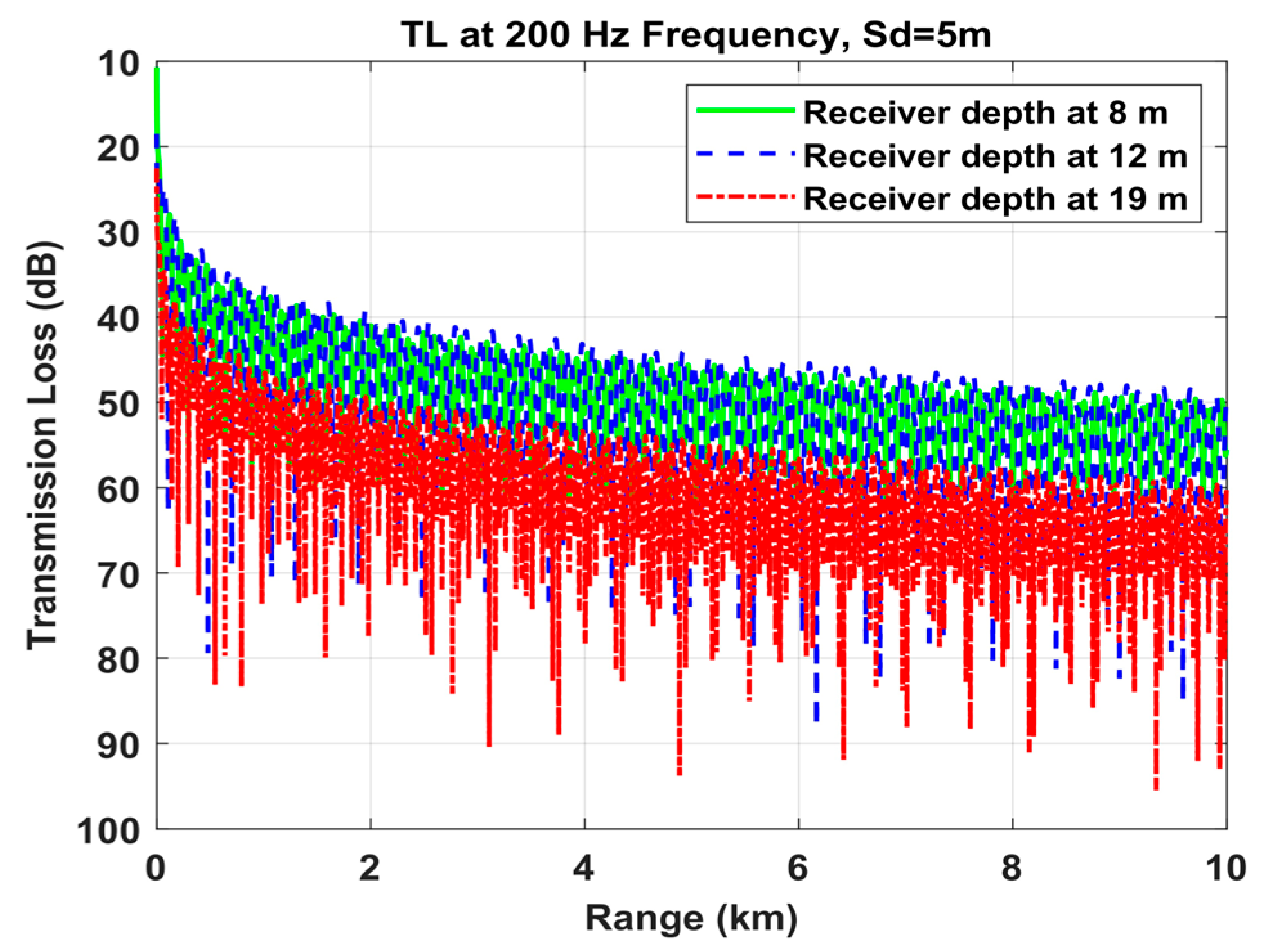
4.2.2. Influence of Source and Receiver Depths

Figure 13 depicts the TL in decibels (dB) as a function of range in kilometers for various receiver depths. To analyze the position of the source and receiver, the source’s frequency was assumed to be 200 Hz and fixed at 5 m. The three receiver depths are represented by the green line at 8 m, the blue dashed line at 12 m, and the red dotted line representing the receiver at a depth of 19 m, which is near the bottom of the clayey silt sediment.

At the beginning (0 km), both the receivers at the depths of 8 m and 12 m exhibit a significant increase in TL. As the range increases, the transmission loss stabilizes and follows a similar trajectory for both depths, indicating that sound propagation and attenuation exhibit similar characteristics. The TL is highest for the receiver located at a depth of 19 m (shown by the red dotted line), indicating a greater level of attenuation near the bottom sediment. Consequently, the presence of clayey silt sediment at the bottom has a substantial impact on the transmission of sound, resulting in increased transmission loss. The variations in TL across different receiver depths emphasize the impact of the water column and sediment characteristics on the transmission of sound. Furthermore, the research report conducted by [20] highlights the significant impact of both the source and receiver on the TL results. This serves as additional evidence to support and validate the information.

4.2.3. Bottom Roughness

The bottom roughness is a crucial factor in underwater acoustic simulations since it directly impacts the scattering and absorption of sound waves. Thus, it is proposed that a single source existed at a depth of 5 m, emitting sound waves at a frequency of 200 Hz. The receiver is located 5 km away from the source at a depth of 5 m. All other environmental parameters remain consistent, as depicted in Figure 6. Figure 14 illustrates the variation in transmission loss for different values of bottom roughness at 0.1 m, 0.3 m, and 0.5 m over a distance of up to 5 km from the described model. The transmission loss increases as the range and bottom roughness increases, as indicated by the green line for 0.1 m, the blue dashed line for 0.3 m, and the red dotted line for 0.5 m. This indicates that the acoustic signal weakens as it travels farther from the source. Moreover, the corresponding result illustrates that the presence of bottom roughness has a significant influence on transmission loss at a frequency of 200 Hz. A sea bottom with a roughness of 0.5 m results in higher transmission loss, particularly when observing longer distances. This information is crucial for underwater acoustic modeling and simulation because it emphasizes the need to consider the roughness of the seabed when making precise predictions about the propagation of acoustic signals.

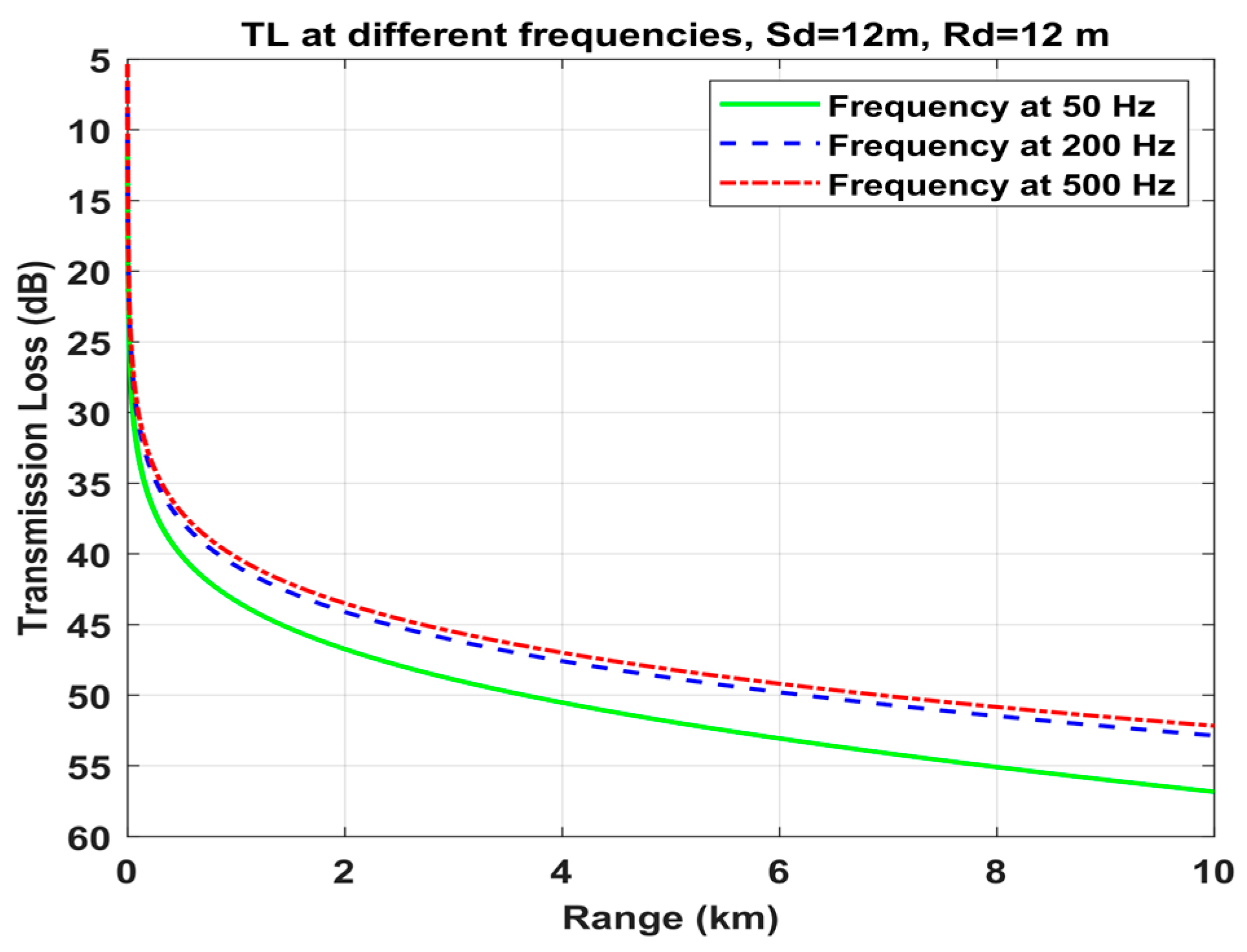
4.2.4. Incoherent Transmission Loss

Incoherent TL is the quantification of the decrease in sound intensity within a water medium without taking into account the phase relationships between various sound waves. The calculation of energy loss in this context involves summing the intensities of the distinct modes, irrespective of their phase. Figure 9 illustrates the coherent transmission loss over a different frequency (50 Hz, 200 Hz, 500 Hz), whereas Figure 13 shows the coherent transmission loss at different receiver depths (8 m, 12 m, 19 m). The results demonstrate the complexity of analysis and display rapid fluctuations caused by mode interference. Hence, this research also takes into account the computation of incoherent transmission loss, using the same parameters of the model for various frequencies and receivers, as depicted in Figure 9 and Figure 13, respectively. The outcomes of incoherent measures are reflected in a more uniform transmission loss curve, as it solely takes into account energy dissipation without the rapid fluctuations caused by interference. Figure 15 and Figure 16 display the incoherent transmission loss for a range-independent environment at different frequencies and receiver depths, respectively. The outcomes of incoherent measures are reflected in a more uniform transmission loss curve, as it solely takes into account energy dissipation without the fast variations induced by interference. Figure 15 and Figure 16 display the incoherent transmission loss for a range-independent environment at different frequencies and receiver depths, respectively.

Figure 15 illustrates the incoherent TL at various frequencies (50 Hz, 200 Hz, and 500 Hz) as a function of distance in kilometers. The source depth (Sd) and receiver depth (Rd) are both set at 12 m. The corresponding results suggest that higher frequencies experience less transmission loss over long distances because they interact less with the bottom compared to lower frequencies, which are more influenced by the properties of the bottom. Figure 16 illustrates the incoherent transmission loss TL at various depths of the receiver while keeping the source depth (Sd) constant at 5 m and the frequency at 200 Hz. The transmission loss at shallower depths (8 m and 12 m) has a similar trajectory for both depths and shows less increase as the range increases. However, the sediment layer experiences more attenuation at a maximum depth of 19 m, which is close to the bottom. When comparing receivers at different depths, the transmission loss is greater for those at 19 m compared to those at 8 and 12 m. This is due to the increased interaction between features in the water column and the sediments at the bottom.

5. Discussion

In this section, acoustic propagation and transmission loss results in shallow water at unexplored sites in the northern Arabian Sea, and these are compared with the internationally published results of various research papers. For comparison purposes, the selected studies follow similar work on acoustic propagation in shallow waters. In our work, we have conducted the simulations to calculate transmission loss, and we use Kraken C to simulate the acoustic data in a shallow water waveguide, which is similar to that of the Arabian Sea environment, as illustrated in Figure 6. The Kraken C program only provides the output file of eigenvalues and eigenfunctions. Subsequently, a dedicated MATLAB code was developed to calculate transmission loss with respect to different frequencies, ranges, source/receiver depths, bottom roughness, etc. The established code can be utilized for further analysis. We calculated and analyzed the propagation loss due to bottom roughness in terms of RMS height variation. Due to the limitation of the Kraken C program, we have considered the RMS height variation as the input parameter in bottom roughness. In this regard, we estimated a roughness value for the Arabian Sea and estimated the RMS height based on available literature. The environment parameters are considered range independent. Here, three layers are considered: the water layer, the sediment layer, and the seafloor half-space. The SSP of the water layer is shown in Figure 4. The physical parameters of the sediment are actually measured and given in Table 1. The acoustic parameters, such as sound velocity and attenuation in the sediment, are measured through experiments at high frequencies by our previous work [23] and extended to lower frequencies. The measured sound speed and attenuation are consistent with the model used by the authors (Shaikh et al. 2024) [23] due to the utilization of the same novel sediment sample of clay silt characteristics. Moreover, due to limitations in exploring the basement of the study site, the bottom properties of the basement are estimated based on available relevant literature. The geo-acoustic parameters are given in Table 2.

It has been depicted in Figure 10 that the corresponding transmission loss of sound in a shallow water environment with a clayey sediment layer is a function of frequency (in Hz) and depth (in meters). Particularly at specific depths, lower frequencies having a range from 50 to 500 Hz experience more significant attenuation, whereas higher frequencies, between 230 Hz and 500 Hz, often exhibit lower transmission loss. The loss in the range is highest at low frequencies, as illustrated in Figure 10. It drops off rapidly as the frequency increases. It was also confirmed by the authors (Sanjana et al.) [22], who studied how environmental factors in coastal seas affect sound propagation.

It has been depicted in Figure 13 that the transmission loss of sound in a shallow water environment is a function of range in kilometers for various receiver depths. The transmission loss is calculated at the three different receiver depths. Two receiver depths are considered above the bottom of the clayey silt sediment, and one is kept near the bottom of the clayey silt sediment. This configuration was set to analyze the effect of receiver depth on transmission loss. The transmission loss is highest for the receiver located at a depth of 19 m, which indicates a greater level of attenuation near the bottom sediment. The variation in TL across different receiver depths highlights the impact of the water column and sediment characteristics on acoustic transmission. It was also confirmed by the authors (Meyer et al.) [20], who conducted the research and highlighted the significant impact of both the source and receiver on the TL results. This serves as evidence to validate our research findings.

Bhatti et al. [14] investigated sound propagation employing normal mode theory in a range-independent shallow water environment, excluding a sediment layer at the bottom. The results demonstrated that transmission loss increases with higher frequencies and decreases with increased receiver depth. In this study, as illustrated in Figure 11 and Figure 15, the transmission loss is reduced with higher frequencies due to the presence of a sediment clay layer in the ocean model. The works of [18,19,22] also assert the same phenomenon. Moreover, as shown in Figure 13, the transmission loss increases with increased receiver depth due to the receiver being positioned near the bottom of clay silt sediment. Meyer et al. [20] also verified the same.

6. Conclusions

This study investigated the acoustic propagation and transmission loss in shallow water at an unexplored site in the northwestern Arabian Sea, close to Pakistan’s coastline. The normal mode Kraken C program was used to perform the simulation results. An ocean model and associated code have been created to compute transmission loss based on various frequencies, distances, source/receiver depths, and bottom roughness. The model results have been compared to the relevant findings of other authors and have been deemed satisfactory. These results have not been previously published for this region. This study also explored the coherent and incoherent transmission loss and its relationship with fluctuations in shallow water, explicitly focusing on the impact of these variations on sound propagation. The simulation results indicate that transmission loss relative to range is higher at low frequencies (50–225 Hz) and reduces at higher frequencies (230–500 Hz). In addition, transmission loss is significantly higher for receivers at 19 m depth than for those at shallower depths (8 m and 12 m). This is the outcome of the receivers being positioned near the layer of bottom sediments. Moreover, a seabed characterized by rougher surfaces leads to increased transmission loss, signifying that the acoustic signal decreases more as the seabed’s roughness increases. The current study encountered certain limitations in its investigation of the basement’s properties, including the complexity of directly measuring parameters such as bottom roughness, sound speed, and attenuation and the constraints associated with the Krakern C software. As a result, these fundamental parameters were estimated using values from relevant literature. In future studies, dedicated efforts will be made to address these gaps by incorporating advanced measurement techniques and software updates to obtain more precise evaluations. These findings will improve the precision of propagation loss modeling and broaden the relevance of the results to real-world scenarios. In addition, this study encompasses a site-specific analysis that may serve as a reference for future research in this unexplored location.

References

1. Venkateswara Rao, C.; Ravi Sankar, M.; SR Charan, P.; Bavya Sri, V.; Bhaavan Sri Sailesh, A.; Sri Uma Suseela, M.; Padmavathy, N. Analysis of acoustic channel model characteristics in deep-sea water. In Proceedings of the International Conference on Cognitive Computing and Cyber Physical Systems, Bhimavaram, India, 26–27 November 2022; Springer: Berlin/Heidelberg, Germany, 2022. [Google Scholar]
2. Zhu, H.; Xue, Y.; Ren, Q.; Liu, X.; Wang, J.; Cui, Z.; Zhang, S.; Fan, H. Inversion of shallow seabed structure and geoacoustic parameters with waveguide characteristic impedance based on Bayesian approach. Front. Mar. Sci. 2023, 10, 1104570. [Google Scholar] [CrossRef]
3. Ewing, J.; Carter, J.A.; Sutton, G.H.; Barstow, N. Shallow water sediment properties derived from high-frequency shear and interface waves. J. Geophys. Res. Solid Earth 1992, 97, 4739–4762. [Google Scholar] [CrossRef]
4. Tolstoy, I.; Clay, C. Ocean acoustics: An evaluation. Rev. Geophys. 1966, 4, 33–40. [Google Scholar] [CrossRef]
5. Su, X.; Qin, J.; Yu, X. Interference Pattern Anomaly of an Acoustic Field Induced by Bottom Elasticity in Shallow Water. J. Mar. Sci. Eng. 2023, 11, 647. [Google Scholar] [CrossRef]
6. Zhang, X.; Wang, Q.; Wang, W.; Zhang, Y.; Yan, H.; Zhu, H. Effects of inclined sea bottom on acoustic propagation characteristics in shallow ocean fronts. In Proceedings of the CAIBDA 2022, 2nd International Conference on Artificial Intelligence, Big Data and Algorithms, Nanjing, China, 17–19 June 2022; VDE: Frankfurt am Main, Germany, 2022. [Google Scholar]
7. Jensen, F.B. Numerical models in underwater acoustics. In Hybrid Formulation of Wave Propagation and Scattering; Springer: Berlin/Heidelberg, Germany, 1984; pp. 295–335. [Google Scholar]
8. Kexin, L.; Chitre, M. Ocean Acoustic Propagation Modeling Using Scientific Machine Learning. In Proceedings of the OCEANS 2021: San Diego–Porto, San Diego, CA, USA, 20–23 September 2021; IEEE: Piscataway, NJ, USA, 2021. [Google Scholar]
9. Pekeris, C.L. Theory of Propagation of Explosive Sound in Shallow Water; Generic Publications: Homebush West, Australia, 1948. [Google Scholar]
10. Jensen, F.; Ferla, M.S. The SACLANTCEN Normal-Mode Acoustic Propagation Model, SACLANTCEN SM-121; SACLANT ASW Research Centre: La Qpezia, Italy, 1979. [Google Scholar]
11. Porter, M.B. The KRAKEN Normal Mode Program; Naval Research Laboratory: Washington, DC, USA, 1992. [Google Scholar]
12. Etter, P.C. Underwater Acoustic Modeling and Simulation; CRC Press: Boca Raton, FL, USA, 2018. [Google Scholar]
13. Jensen, F.B.; Kuperman, W.A.; Porter, M.B.; Schmidt, H. Normal Modes. In Computational Ocean Acoustics; Springer: New York, NY, USA, 2011; pp. 337–455. [Google Scholar]
14. Bhatti, A.A.; Khan, S.; Yiwang, H. Numerical Simulation of Shallow Water Propagation using Normal Mode Theory. In Proceedings of the 2019 16th International Bhurban Conference on Applied Sciences and Technology (IBCAST), Islamabad, Pakistan, 8–12 January 2019; IEEE: Piscataway, NJ, USA, 2019. [Google Scholar]
15. Shaikh, S.; Huang, Y.W. Influences analysis of environmental parameters on sound propagation in shallow water. Appl. Mech. Mater. 2014, 556, 4815–4819. [Google Scholar] [CrossRef]
16. Jensen, F.B.; Kuperman, W.A.; Porter, M.B.; Schmidt, H.; McKay, S. Computational ocean acoustics. Comput. Phys. 1995, 9, 55–56. [Google Scholar] [CrossRef]
17. Valle-Molina, C.; Stokoe, K.H. Seismic measurements in sand specimens with varying degrees of saturation using piezoelectric transducers. Can. Geotech. J. 2012, 49, 671–685. [Google Scholar] [CrossRef]
18. Rogers, A.K.; Yamamoto, T.; Carey, W. Experimental investigation of sediment effect on acoustic wave propagation in the shallow ocean. J. Acoust. Soc. Am. 1993, 93, 1747–1761. [Google Scholar] [CrossRef]
19. Noufal, K.; Sanjana, M.; Latha, G. Acoustic propagation in shallow waters of south east Arabian Sea using Normal mode approach. Indian J. Geo Mar. Sci. 2017, 46, 2175–2181. [Google Scholar]
20. Meyer, V.; Audoly, C. A comparison between experiments and simulation for shallow water short range acoustic propagation. In Proceedings of the ICSV 24 24th International Congress on Sound and Vibration, London, UK, 23–27 July 2017. [Google Scholar]
21. Bonnel, J.; Flamant, J.; Dall’Osto, D.R.; Le Bihan, N.; Dahl, P.H. Polarization of ocean acoustic normal modes. J. Acoust. Soc. Am. 2021, 150, 1897–1911. [Google Scholar] [CrossRef]
22. Sanjana, M.; Latha, G.; Thirunavukkarasu, A.; Raguraman, G. Acoustic propagation affected by environmental parameters in coastal waters. Indian J. Geo Mar. Sci. 2014, 43, 17–21. [Google Scholar]
23. Shaikh, S.; Huang, Y.-W.; Zhang, Z.-C.; Zuberi, H.H. Fine Sand and Clay Sediment Acoustic Properties of the Novel Sediment Sample from the Arabian Sea: Experimental Investigations and Biot–Stoll Model Validation. China Ocean Eng. 2024, 38, 169–180. [Google Scholar] [CrossRef]
24. Folk, R.L. Petrology of Sedimentary Rocks; Hemphill Publishing Company: Sutton, UK, 1980. [Google Scholar]
25. Kimura, M. Prediction of tortuosity, permeability, and pore radius of water-saturated unconsolidated glass beads and sands. J. Acoust. Soc. Am. 2018, 143, 3154–3168. [Google Scholar] [CrossRef] [PubMed]
26. Udden, J.A. Mechanical composition of clastic sediments. Bull. Geol. Soc. Am. 1914, 25, 655–744. [Google Scholar] [CrossRef]
27. Wentworth, C.K. A scale of grade and class terms for clastic sediments. J. Geol. 1922, 30, 377–392. [Google Scholar] [CrossRef]
28. Jackson, D.; Richardson, M. High-Frequency Seafloor Acoustics; Springer Science & Business Media: Cham, Switzerland, 2007. [Google Scholar]
29. Avnimelech, Y.; Ritvo, G.; Meijer, L.E.; Kochba, M. Water content, organic carbon and dry bulk density in flooded sediments. Aquac. Eng. 2001, 25, 25–33. [Google Scholar] [CrossRef]
30. Yu, S. Geoacoustic Parameter Inversion Based on Backscattering Strength; Harbin Engineering University: Harbin, China, 2014; (In Chinese with an English Abstract). [Google Scholar]
31. Danielson, R.; Sutherland, P. Porosity. In Methods of Soil Analysis: Part 1 Physical and Mineralogical Methods; American Society of Agronomy, Inc.: Madison, WI, USA, 1986; Volume 5, pp. 443–461. [Google Scholar]
32. Azeez, A.; Revichandran, C.; Muraleedharan, K.; John, S.; Seena, G.; Nair, R.C.; Manju, K. Sound speed variation in the coastal waters off Cochin and signature of subsurface maxima. Ocean Dyn. 2021, 71, 923–933. [Google Scholar]
33. Qiao, G.; Ismail, A.; Aatiq, M. A Study on Multi-Path Channel Response of Acoustic Propagation in Northwestern Arabian Sea. Res. J. Appl. Sci. Eng. Technol. 2013, 4619–4628. [Google Scholar] [CrossRef]
34. Mackenzie, K.V. Nine-term equation for sound speed in the oceans. J. Acoust. Soc. Am. 1981, 70, 807–812. [Google Scholar] [CrossRef]
35. Ismail, A.; Gang, Q.; Khan, R.; Kabir, J.; Pasha, B.; Masood, A.; Malik, A.; Khan, A. Variability of channel response and acoustic system performance: Simulation study. In Proceedings of the 2013 10th International Bhurban Conference on Applied Sciences & Technology (IBCAST), Islamabad, Pakistan, 15–19 January 2013; IEEE: Piscataway, NJ, USA, 2013. [Google Scholar]
36. Frisk, G.V. Ocean and Seabed Acoustics: A Theory of Wave Propagation; Pearson Education: London, UK, 1994. [Google Scholar]
37. Ma, X.; Wang, Y.; Zhu, X.; Liu, W.; Lan, Q.; Xiao, W. A spectral method for two-dimensional ocean acoustic propagation. J. Mar. Sci. Eng. 2021, 9, 892. [Google Scholar] [CrossRef]
38. Ma, X.; Wang, Y.; Zhu, X.; Liu, W.; Xiao, W.; Lan, Q. A high-efficiency spectral method for two-dimensional ocean acoustic propagation calculations. Entropy 2021, 23, 1227. [Google Scholar] [CrossRef] [PubMed]
39. Ahmed Alanazi, M.; Ali, I. Simulations and analysis of underwater acoustic wave propagation model based on Helmholtz equation. Appl. Math. Sci. Eng. 2024, 32, 2338397. [Google Scholar] [CrossRef]
40. Zhao, Y.; Wang, M.; Xue, H.; Gong, Y.; Qiu, B. Prediction method of underwater acoustic transmission loss based on deep belief net neural network. Appl. Sci. 2021, 11, 4896. [Google Scholar] [CrossRef]
Figure 1. Study site in shallow water of the northern Arabian Sea.
Jmse 12 02256 g001
Figure 2. Temperature data for northern Arabian Sea.
Jmse 12 02256 g002
Figure 3. Salinity data for northern Arabian Sea.
Jmse 12 02256 g003
Figure 4. SSP for northern Arabian Sea.
Jmse 12 02256 g004
Figure 5. Block diagram of normal mode theory.
Jmse 12 02256 g005
Figure 6. Ocean shallow water environment.
Jmse 12 02256 g006
Figure 7. Sound speed in clayey silt sediment.
Jmse 12 02256 g007
Figure 8. Attenuation in clayey silt sediment.
Jmse 12 02256 g008
Figure 9. TL for different frequencies.
Jmse 12 02256 g009
Figure 10. Transmission loss for 2.0 km range.
Jmse 12 02256 g010
Figure 11. TL versus range for low and high-frequency waves.
Jmse 12 02256 g011
Figure 12. TL for frequencies of 50–500 Hz.
Jmse 12 02256 g012
Figure 13. Variation in TL with different receiver depths.
Jmse 12 02256 g013
Figure 14. TL for different bottom roughness.
Jmse 12 02256 g014
Figure 15. Incoherent TL at different frequencies.
Jmse 12 02256 g015
Figure 16. Incoherent TL at different receiver depths.
Jmse 12 02256 g016