Article

Comparison of Collision Avoidance Algorithms for Unmanned Surface Vehicle Through Free-Running Test: Collision Risk Index, Artificial Potential Field, and Safety Zone

1
Department of Marine Design Convergence Engineering, Pukyong National University, Busan 48513, Republic of Korea
2
Autonomous Ship Verification & Evaluation Research Center, Korea Research Institute of Ships and Ocean Engineering (KRISO), Ulsan 44539, Republic of Korea
3
Maneuvering Control Research Team, Avikus, Seoul 06236, Republic of Korea
4
Korea Research Institute of Ships and Ocean Engineering (KRISO), Deajeon 34103, Republic of Korea
5
Department of Naval Architecture and Marine Systems Engineering, Pukyong National University, Busan 48513, Republic of Korea
6
Future Innovation Institue, Seoul National University, Seoul 08826, Republic of Korea
*
Author to whom correspondence should be addressed.
J. Mar. Sci. Eng. 2024, 12(12), 2255; https://doi.org/10.3390/jmse12122255
Submission received: 31 October 2024 / Revised: 27 November 2024 / Accepted: 4 December 2024 / Published: 9 December 2024
(This article belongs to the Special Issue Unmanned Marine Vehicles: Navigation, Control and Sensing)

Abstract

:
This paper details the development of a collision avoidance algorithm for unmanned surface vehicles (USVs) and its validation using free-running tests. The USV, designed as a catamaran, incorporates a variety of sensors for its guidance, navigation, and control system. It performs turning maneuvers using thrusters positioned on the port and starboard sides. The robot operating system is used to streamline communication, transmitting data such as position, orientation, and situational information from diverse sensors. Using the collision risk index (CRI) method, the algorithm calculates risk based on the distance to obstacles and the angle to the desired waypoint, directing the USV on a path with minimized risk. Noise within the data captured by the two-dimensional light detection and ranging system is filtered out using the k-dimensional tree and Euclidean distance methods, ensuring single obstacles are distinctly identified. To assess the efficacy of the CRI-based collision avoidance algorithm, it was benchmarked against other algorithms rooted in the artificial potential field and safety zone methods within an artificial tank setting. The results highlight the CRI method’s superior time efficiency and optimality in comparison to its counterparts.

1. Introduction

Recent advances in autonomous technology have underscored the diverse roles and applications of unmanned surface vehicles (USVs) within the maritime domain. More than ever, USVs play important roles in marine environmental monitoring, oceanographic studies, structural inspections, maritime surveillance, and patrols. Numerous studies focused on enhancing the guidance, navigation, and control systems of USVs have been conducted. Significant contributions include advances in guidance and control performance, collision avoidance technique refinement, developments in autonomous berthing/unberthing, and the optimization of swarm operations [1,2]. Of these areas, collision avoidance is pivotal in ensuring the safe execution of diverse USV missions.
Research on maritime collision avoidance predominantly focuses on algorithms for USVs, such as the velocity obstacle (VO) [3], artificial potential field (APF) [4,5], the dynamic window approach [6,7,8], and deep reinforcement learning [9]. However, Chen et al. (2023) [10] highlighted certain limitations in these algorithms, such as assumptions that target ships maintain their speed and course and scenarios where vessels might fall into local minima.
Given these limitations, recent studies have sought solutions, verifying their findings through simulations. Cho et al. (2022) [11] introduced a probabilistic VO algorithm tailored for encounters with vessels violating international regulations for preventing collisions at sea and validated it using Monte Carlo simulations. Jo et al. (2022) [1] compared the VO algorithm to the biased APF in simulations of USV swarm operations during formation changes. Meanwhile, Ko et al. (2022) [12] integrated the VO-based collision avoidance algorithm with the maneuvering modeling group for simulations, focusing on ship collision avoidance in wavy conditions. Lee and Woo (2023) [13] proposed a reactive collision avoidance algorithm utilizing a Gaussian mixture model and motion primitives, validated through simulations with USV.
To comprehensively validate the performance of collision avoidance algorithms, it is imperative to conduct both field tests and free-running tests. Woo and Kim (2020) [14] introduced a deep-reinforcement-learning-based method tailored to the decision-making stage for USVs, demonstrating its efficacy through free-running tests using virtual constant VO models. Similarly, Han et al. (2020) [15] conducted field experiments on the USV Aragon, equipping it with several sensors such as radar, light detection and ranging (LiDAR), and cameras to validate its autonomous navigation and collision avoidance capabilities. LiDAR uses the time-of-flight method to measure properties like distance and velocity based on the return time of a laser pulse. As a result, LiDAR data are collected in the form of a list, containing distance data for each angle of resolution, ranging from 0 to 360°. Recognizing the benefits of such sensors, researchers including Jo et al. (2021) [16], Kim et al. (2022) [17], and Gonzalez-Garcia et al. (2022) [18] have integrated LiDAR into their platforms and then undertook field tests with USVs.
Several researchers use simulations to validate algorithms; however, a significant disparity between simulations and model tests exists. These differences can arise from modeling errors in the simulations or environmental disturbances. Additionally, this approach assumes that the algorithm establishes an avoidance path based on the relative relationship between the vessel and the target or obstacles under ideal conditions of reliability, connectivity, and stability. Moreover, many studies on collision avoidance tend to focus on the performance of a single algorithm without comparative analysis with others. While there has been extensive research on collision avoidance algorithms, direct comparisons of their performance remain limited. This study was designed to address this gap by evaluating the strengths and weaknesses of well-known algorithms, prior research, and a newly proposed algorithm.
This study focused on the development of a USV equipped with an autonomous guidance, navigation, and control (GNC) system for obstacle avoidance. To facilitate autonomous operation, the USV was equipped with several hardware components and software algorithms. Collision avoidance algorithms were developed based on three distinct methods: the APF, safety zone, and collision risk index (CRI) methods. The study selected these algorithms for comparison due to their unique characteristics. APF is a widely used algorithm known for its simplicity and ease of implementation, making it a suitable baseline. The safety zone method, proposed in our previous research (Jo et al., 2021) [16], has demonstrated its effectiveness in LiDAR-based USV obstacle avoidance. CRI, newly developed in this study, evaluates collision risk by considering both the distance to obstacles and the angle to the desired waypoint. The performances of these algorithms are demonstrated and compared using free-running tests in an artificial tank under the same environmental conditions. These experiments showed clearly that the CRI method was the most effective of the three algorithms tested.
The remainder of this paper is organized as follows. In Section 2, the hardware and software systems of the USV used in this work are explained. The GNC system of the USV and the methodologies used for each collision avoidance algorithm are then described. In Section 3, the results of free-running tests conducted with the same USV and environment using each collision avoidance algorithm are presented, combined with a comparison of these results. Section 4 presents the conclusions of this study and future research directions.

2. Materials and Methods

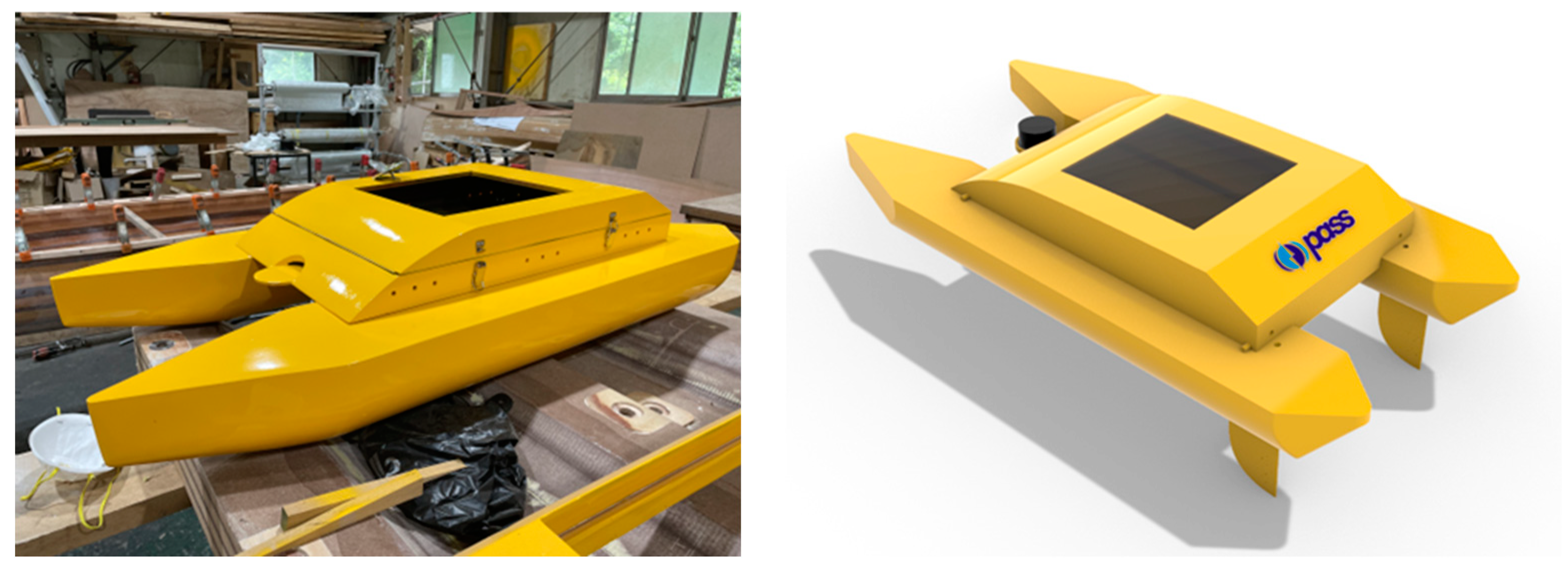
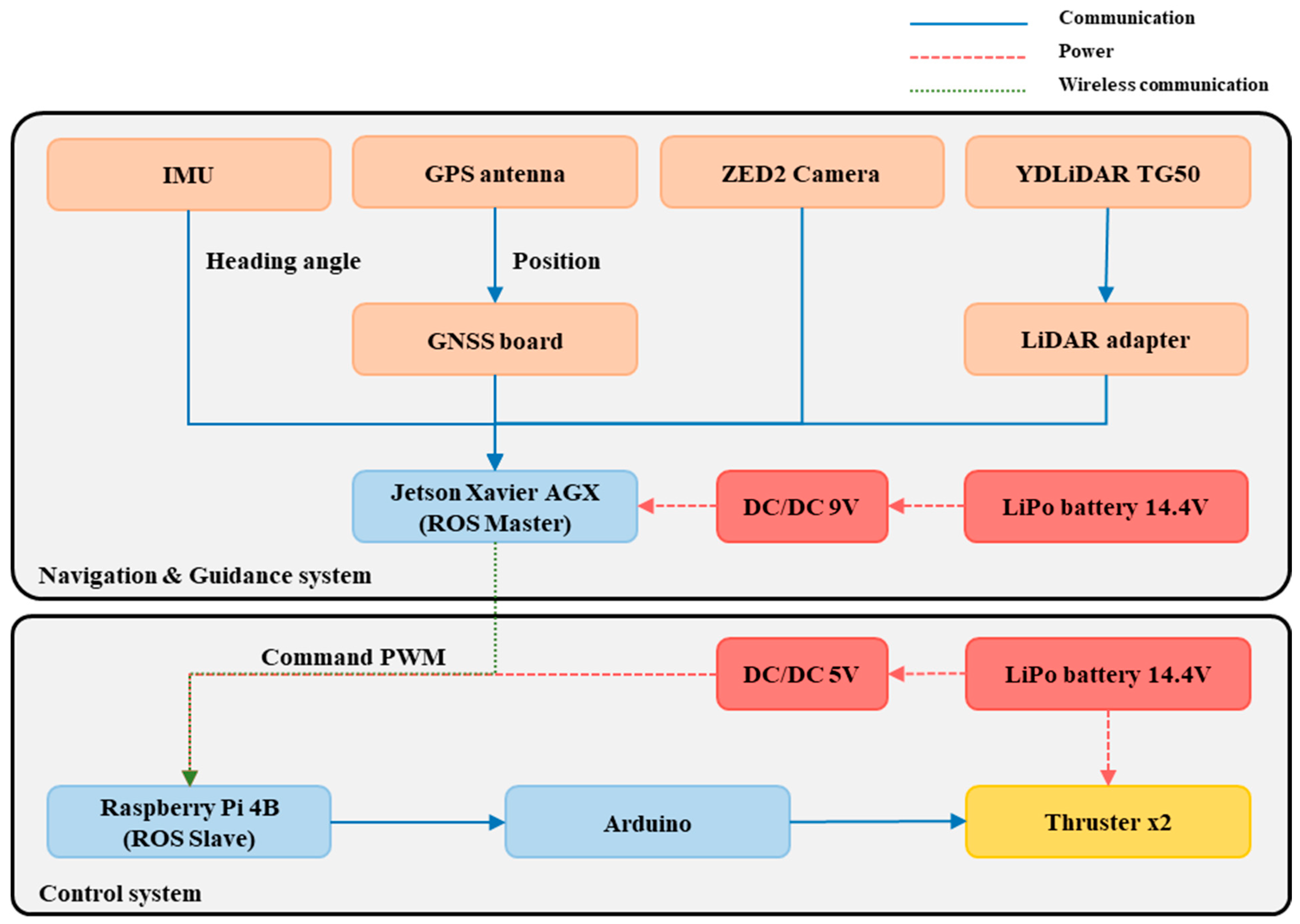
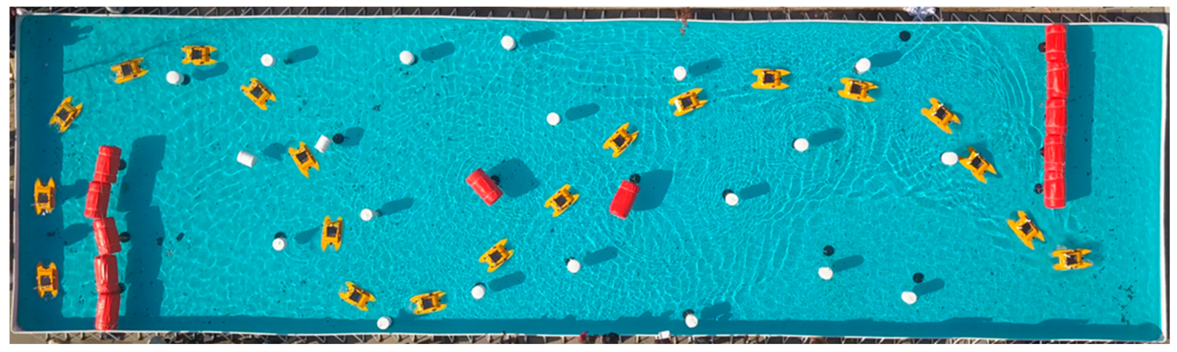
2.1. Hardware System

Figure 1 shows the USV, named the Pukyong Autonomous Surface Ship Mark 2 (PASS Mk II). Designed as a catamaran-type hull platform, it features two propellers, one each on the port and starboard sides. The catamaran design offers enhanced stability and maneuverability, which are critical for effective collision avoidance in dynamic environments. The USV is equipped with a global positioning system (GPS) and an inertial measurement unit (IMU) for precise position measurement, enabling accurate navigation and reducing errors during high-speed maneuvers. A 2D LiDAR system and a camera provide environmental perception, facilitating real-time obstacle detection and avoidance. To facilitate autonomous navigation, the USV houses a main processor for gathering and processing sensor data and a sub-processor governing the propulsion system. Table 1 summarizes the USV’s specifications, including its sensors and processors. Figure 2 illustrates the USV’s composition, highlighting its navigation and guidance systems with main processors and sensors, alongside its control system with two thrusters and a controller.

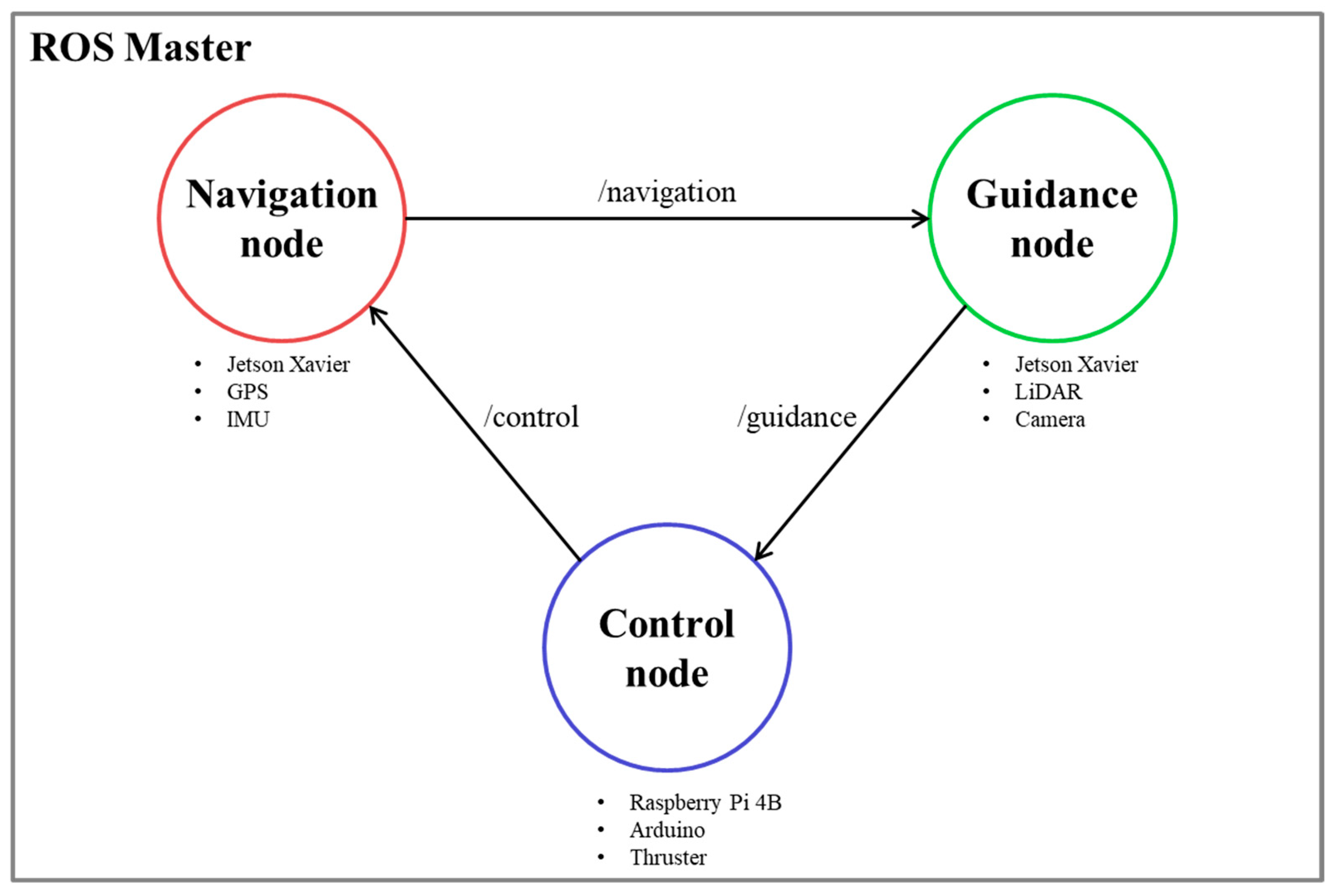
2.2. Software System

Ubuntu and the robot operating system (ROS) were used to integrate sensor data for the control of the autonomous navigation USV. ROS serves as a software framework that streamlines the development, management, and deployment of diverse robotic software applications. It supports multiple programming languages, making it easier for different systems to communicate. Within ROS, the “ROS master” acts as a central manager, while “nodes” perform specific computational processes. By registering nodes with the ROS master, they can exchange messages through topics or services.
The system onboard the USV was composed of three primary ROS nodes. First, the “navigation node” processed sensor data from GPS and IMU to determine the USV’s current position and heading. Second, the “guidance node” analyzed environmental data from LiDAR and the camera to calculate the optimal collision-free route and waypoints. Finally, the “control node” generated low-level commands for the propulsion systems based on the data from the other nodes, ensuring stable and precise maneuvering.
Data communication and processing between these three nodes were carried out through dedicated ROS topics. The “navigation node” published position and heading information via the “/navigation” topic, which the “guidance node” utilized to provide route and waypoint data through the “/guidance” topic. Based on this information, the “control node” executed propulsion and steering commands through the “/control” topic.
The overall system architecture is illustrated in Figure 3, which provides a comprehensive overview of how the nodes (navigation node, guidance node, and control node) interact with each other through dedicated ROS topics (/navigation, /guidance, /control). This figure highlights the data flow between the nodes and the modular structure of the USV’s autonomous framework.

2.3. Collision Avoidance Algorithm

The USV used the GNC system to execute its mission. The GNC unit determined the desired heading angle ψ d to help the USV reach the goal waypoint and avoid obstacles. The navigation unit provided spatial information regarding the USV’s position and orientation. The control unit modulated the thrusters, ensuring the USV accurately aligned with ψ d .
The primary focus was on collision avoidance algorithms within the guidance framework to mitigate collision risks. The collision avoidance algorithms were developed based on the APF, safety zone, and CRI methods. The APF method is a simple and widely used algorithm that guides the USV by moving it from high-potential (obstacle) areas to low-potential (goal) areas. The Safety Zone method, proposed by Jo et al. (2021) [16], identifies and avoids obstacles using LiDAR data based on minimum data count and distance thresholds. The CRI method, developed in this study, evaluates the combined risks of distance and angle to determine the optimal low-risk path for the USV. These theoretical foundations were integrated into the guidance framework and refined through practical implementation, with detailed descriptions provided in the subsequent sections.

2.3.1. Guidance and Control Algorithm
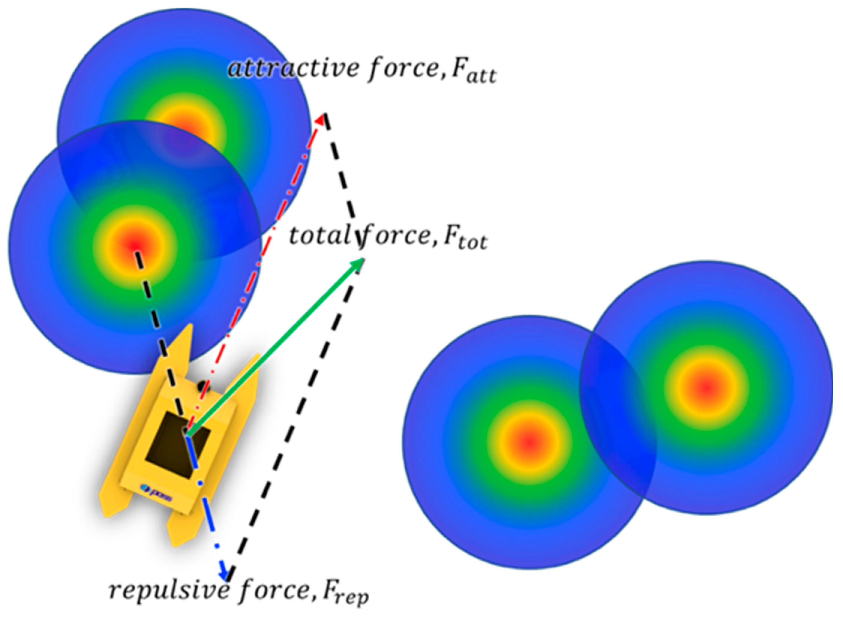
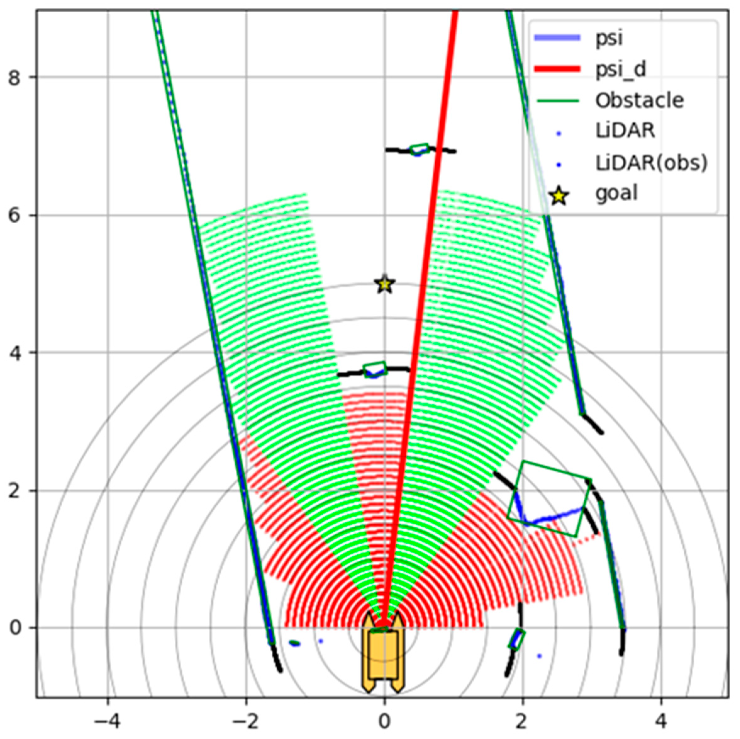
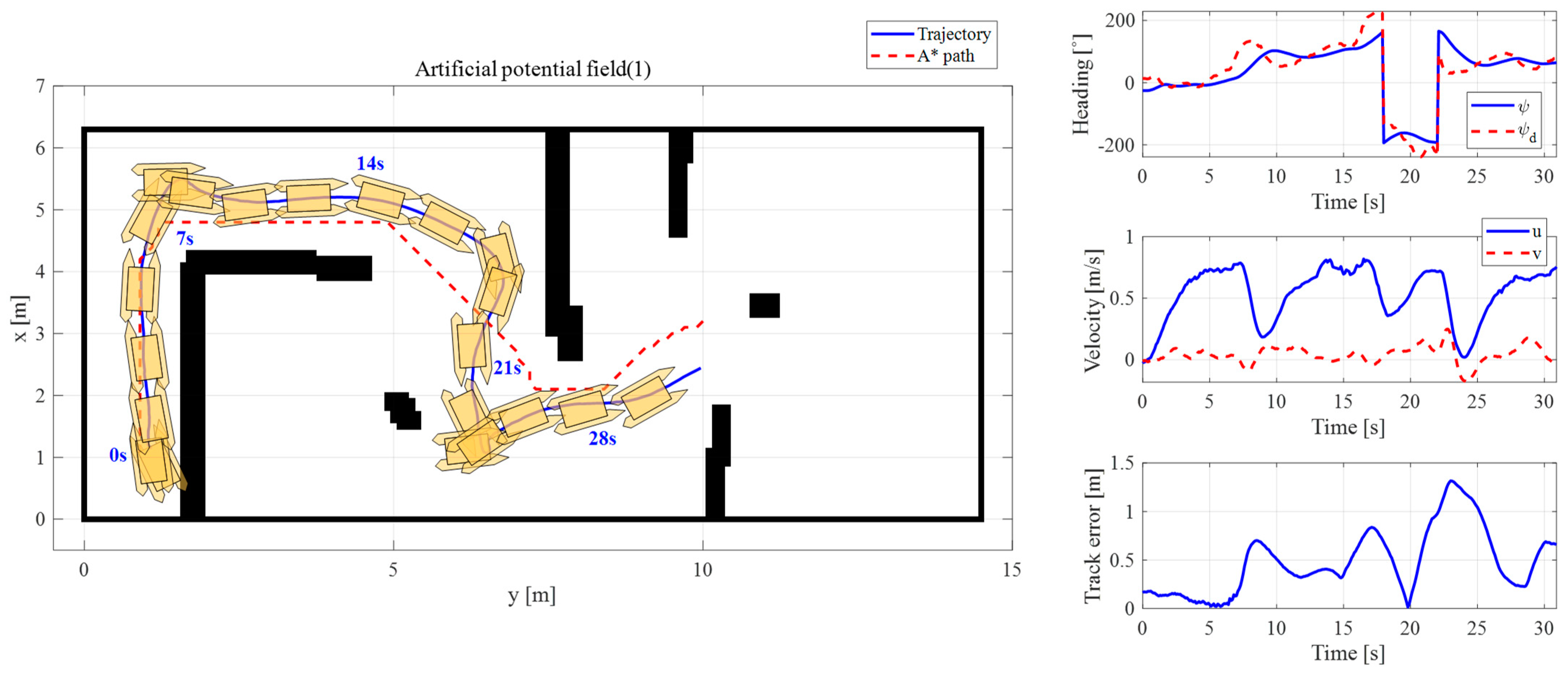
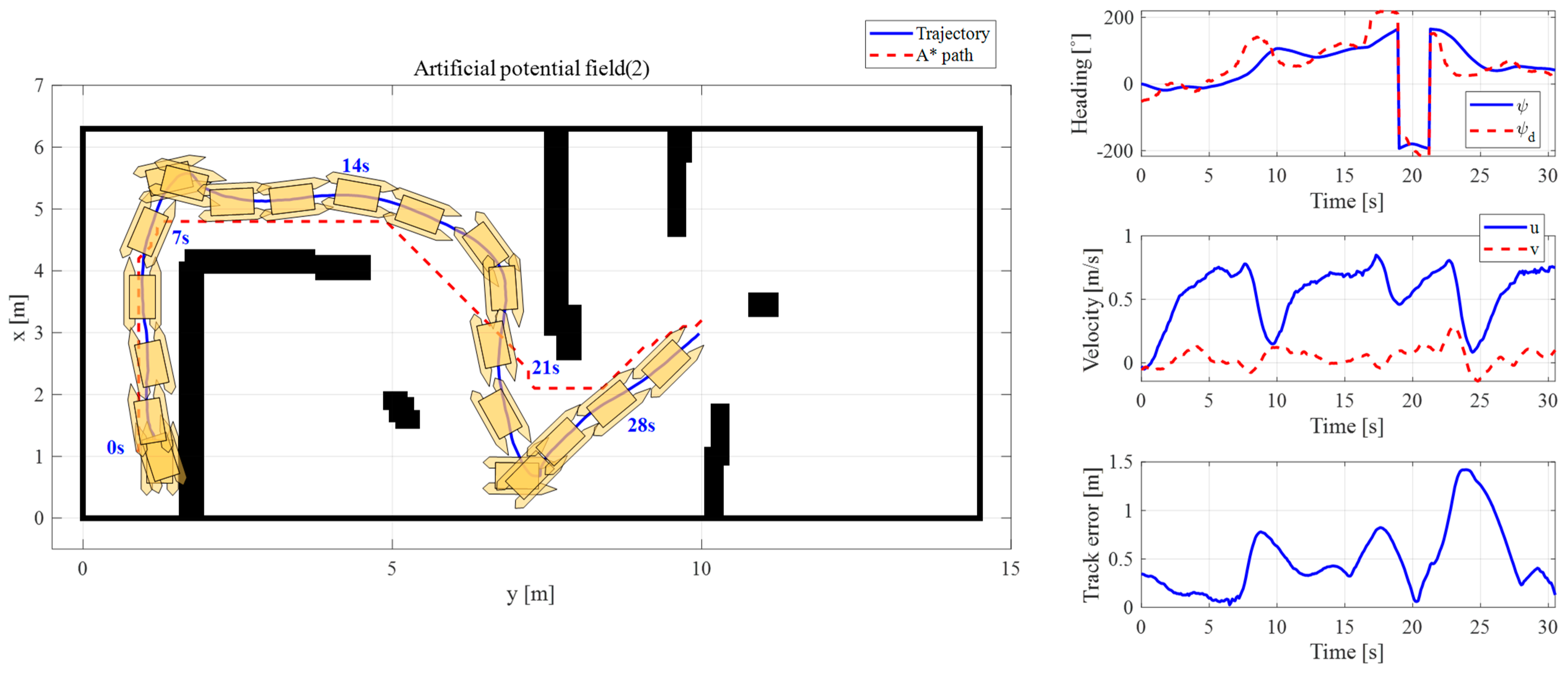
To describe the USV’s horizontal motion, two coordinate systems are used: the earth-fixed O o x o y o and the USV-fixed O x y , as illustrated in Figure 4 [19]. In the earth-fixed system, x o and y o are the north and east directions, respectively, while in the USV-fixed system, x and y are the longitudinal and lateral directions, respectively. The USV’s position in the earth-fixed system is represented by x s and y s . The surge, sway velocities, and overall speed are depicted by variables u , v , and V , respectively. The heading angle ψ is defined by the angle between the x o -axis and the x -axis, where the clockwise direction is positive. T p o r t and T s t b d are the propulsion forces of the port and starboard thrusters, respectively.
The kinematic model of the USV is defined by Equation (1) [19]:
η ˙ = R η ν ,
where R , η, and ν are the transformation matrix, position, and velocity vectors, respectively, as defined in Equations (2)–(4).
R = c o s ψ s i n ψ 0 s i n ψ c o s ψ 0 0 0 1
η = x y ψ T
ν = u v r T
The dynamic model of the USV is defined in Equation (5), where M is the mass matrix, (ν) is the Coriolis and centripetal force matrix, D(ν) is the damping matrix, and τ is the force and moment generated by the thrusters, respectively.
M ν ˙ + C ν ν + D ν ν = τ ,
The angle ψ d toward the waypoint ( x W P , y W P ) is determined using the line-of-sight method as given by Equation (6).
ψ d = tan 1 ( y W P y s ) ( x W P x s )
The proportional-derivative (PD) control method was used, as represented in Equation (7).
n = k p e + k d e ˙ ,     w h e r e   e = ψ d ψ ,
where e is the error between the ψ d and ψ , and n is the output of the controller, which corresponds to the pulse width modulation (PWM) of the thrusters. The values of k p and k d are the control gains for the PD control and are determined through trial and error. The PWM values for the port and starboard thrusters are expressed by Equation (8).
n s t b d = n 0 n ,   n p o r t = n 0 ± n ,
where n p o r t and n s t b d represent the PWM of the port and starboard thrusters, respectively. The maximum and minimum values for n p o r t and n s t b d are 1900 and 1100, respectively, with the thrust being zero at the midpoint where the PWM is set as 1500. n0 means the basic PWM corresponding to the USV’s speed and is determined based on the distance between the USV and obstacles.

2.3.2. APF Method

The APF is one of the algorithms widely used in different domains due to its simplicity and ease of implementation. In the domain of obstacle avoidance, obstacles are assigned high potential, and the goal waypoint is assigned low potential. The APF method guides the USV to move from areas of high potential to areas of low potential, thereby avoiding collisions with obstacles. Figure 5 illustrates the concept of the potential field graphically.
An attractive force F a t t is generated toward the destination, and a repulsive force F r e p is produced from obstacles. The USV moves in the direction of the total force vector F t o t , which is the sum of F a t t and F r e p as described in Equation (9). This movement helps the USV avoid collisions. F a t t and F r e p are calculated as per Equations (10) and (11), respectively.
F t o t = F a t t + F r e p
F a t t = d L O S ,   w h e r e   d L O S = p s p L O S
F r e p = a l n b d r e l ,   w h e r e   d r e l = p o b s p s ,
where p s , p o b s , and p L O S are the locations of the USV, obstacle, and goal waypoint, respectively. For the repulsive force, a logarithmic function was used. Figure 6 shows the potential field based on data measured with LiDAR. Assuming the LiDAR data represents obstacles, a high potential is evident.

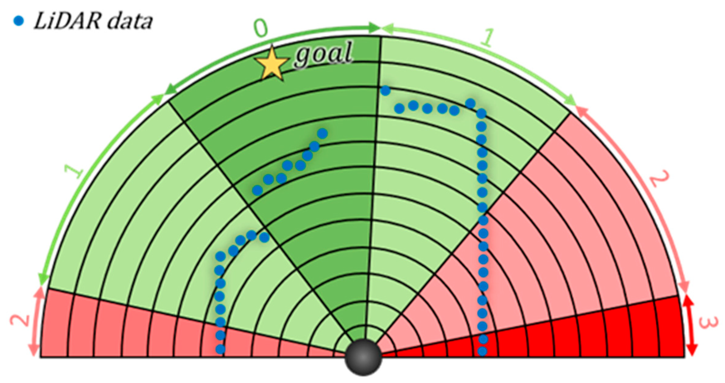
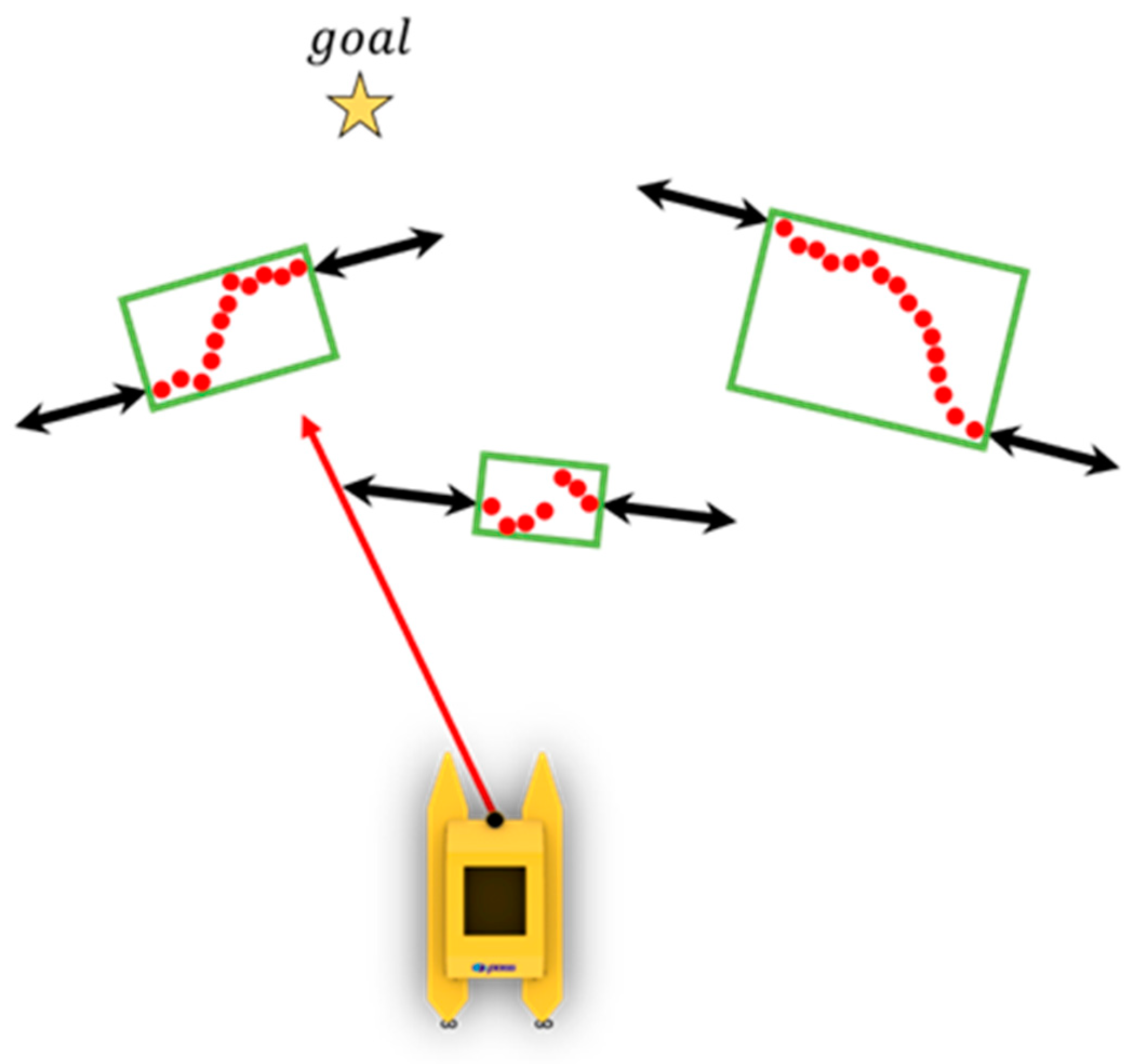
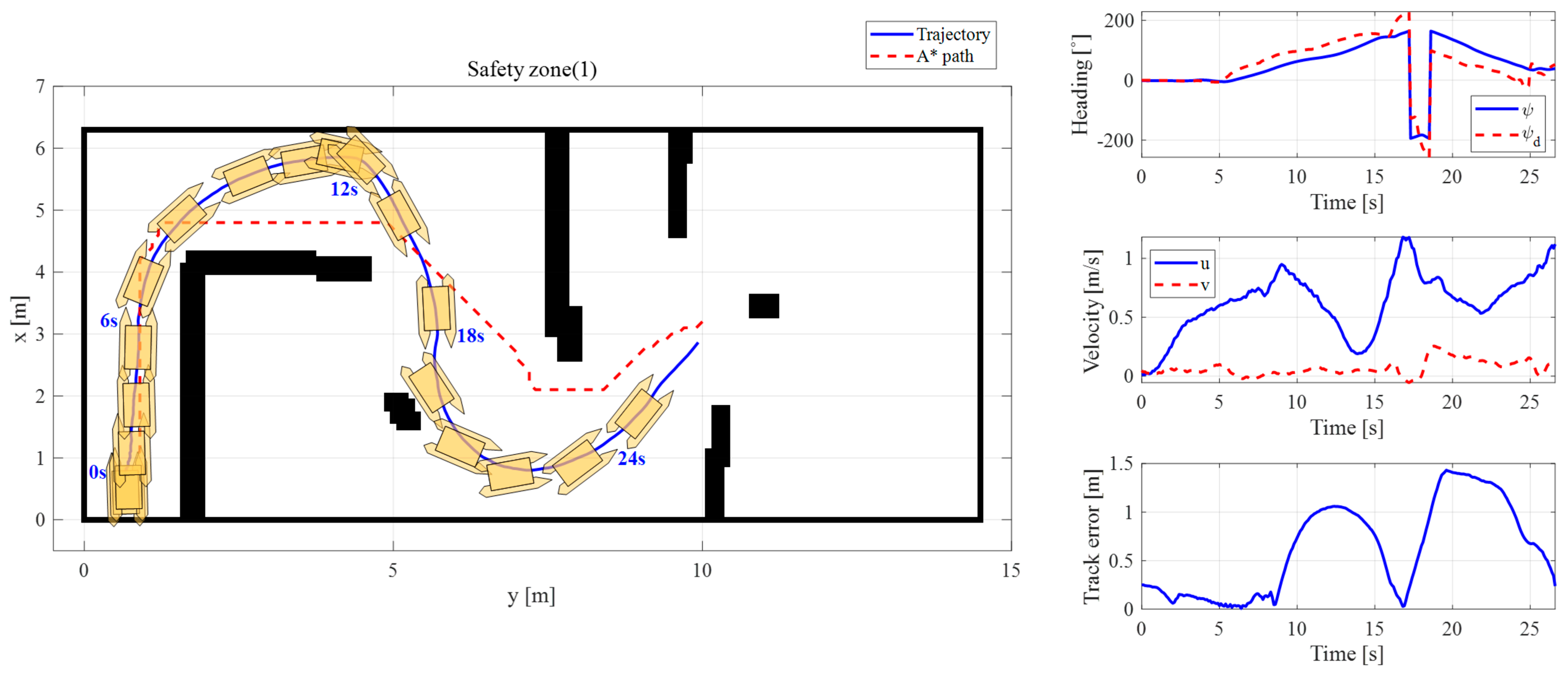
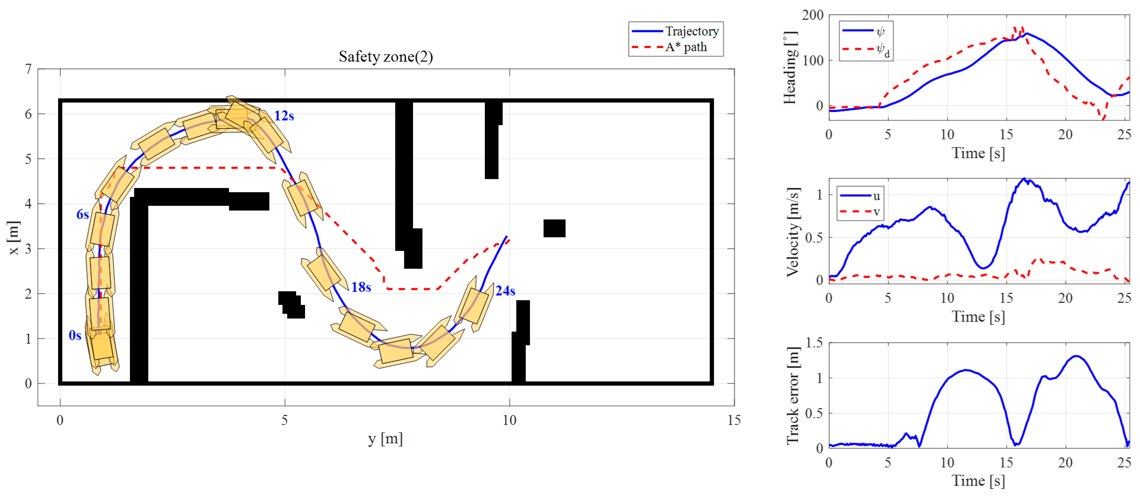
2.3.3. Safety Zone Method
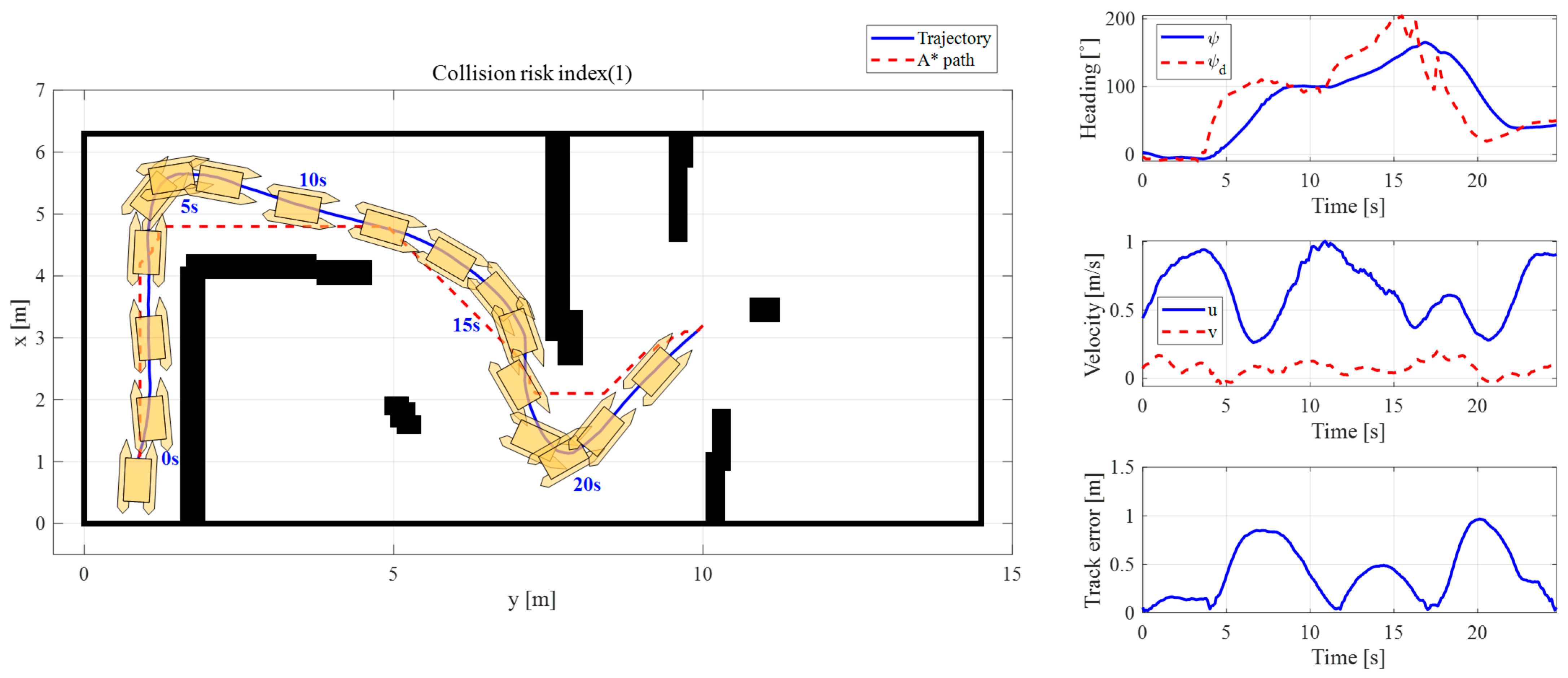
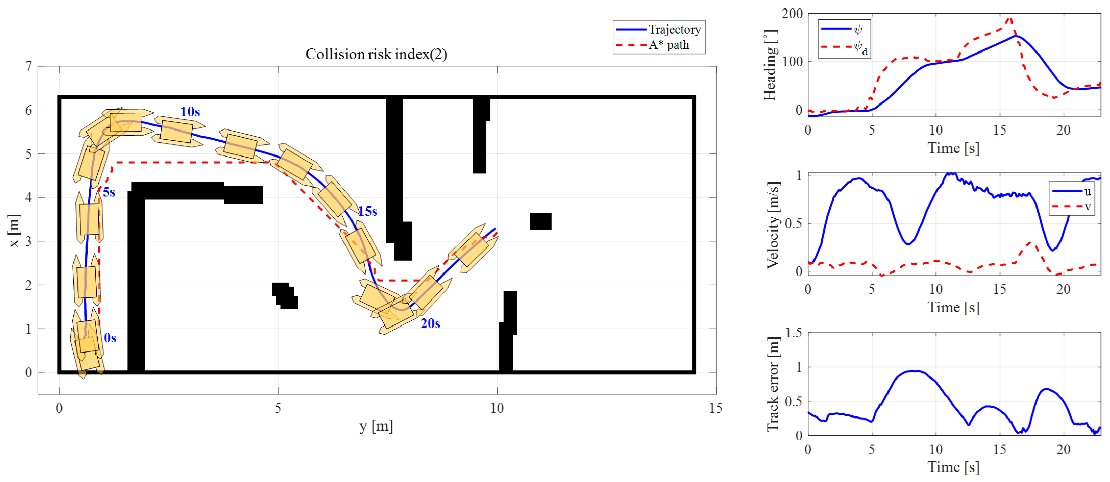
The safety zone method was designed for the autonomous algorithms of a LiDAR-based USV and comprises obstacle recognition and obstacle avoidance stages. In the obstacle recognition stage, the minimum count of LiDAR data and the distance threshold are represented by ηi and ηd, respectively. The average distance for the obstacle data index, ranging from “st” to “ed” as gauged by the LiDAR sensor, is denoted as d ¯ . Figure 7 depicts scenarios where one and two obstacles are identified.
Recognized obstacles are represented by o b s i in Equation (12). o b s i is the i-th obstacle, while α s t and α e d indicate the starting and ending angles, respectively.
o b s i = [ α s t , α e d , d ¯ ]
Based on the recognized obstacles, the safety zone is described according to Equation (13) and is depicted in Figure 8.
s a f e t y   z o n e i = [ θ s t , θ e d , d ¯ s t , d ¯ e d ]
The term “ s a f e t y   z o n e i ” represents the widest zone among the safety zones, and θ s t , θ e d , d ¯ st, and d ¯ ed are the starting angle, ending angle, average distance of obstacles in the direction of the starting angle, and average distance of obstacles in the direction of the ending angle, respectively. The safety zone is then determined according to Equation (14), using the distance to obstacles existing on both sides of the safety zone as weights to safely avoid obstacles.
ψ d = θ s t d ¯ e d + θ e d d ¯ s t d ¯ s t + d ¯ e d

2.3.4. CRI Method

The CRI method is a collision avoidance algorithm that uses the USV’s LiDAR to determine risk based on both the distance to obstacles and the angle to the goal waypoint. This risk comprises two components: distance and angle. The risk associated with distance pertains to avoiding different obstacles, while the risk related to angle provides guidance toward the goal waypoint. After calculating both the distance and angle risk indices, the method directs the USV at an angle ψ d along the path considered to have the lowest risk.
Figure 9 depicts the obstacle recognition process, which precedes the calculation of the distance and angle risk indices. For obstacle recognition, both the Euclidean clustering and the k-dimensional (KD)-tree methods were used. The Euclidean clustering method calculates the distance between two points, grouping them into the same cluster if the distance is less than a certain threshold. The KD-tree, on the other hand, is a binary search tree optimized for storing and querying points in KD space, allowing for the effective and rapid computation of distances to the nearest point. For each point p i , the algorithm identifies its closest k neighbors, where k is set based on the number of adjacent points specified by the user. The average distance between p i and its closest k neighbors, denoted as μ i , is computed using Equation (15):
μ i = 1 k j = 1 k d i s t ( p i , p j ) = 1 k j = 1 k ( x p i x p j ) 2 + ( y p i y p j ) 2
The variance σ i 2 of the difference between the distances is calculated using μ i as per Equation (16).
σ i 2 = 1 k 1 j 1 k ( d i s t p i , p j μ i ) 2
If σ i 2 does not lie within the threshold of variance τ v as defined in Equation (17), then the point is considered an outlier and is removed, as shown in Figure 9A.
p i n o i s e i f   σ i 2 τ v p i = n o i s e i f   σ i 2 > τ v
After the outlier is removed, the distance between p i and p i + 1 , denoted as d p i , less than the threshold of the points’ distance τ p are bundled into one block as in Equations (18) and (19), as shown in Figure 9B,C.
d p i = ( x p i + 1 x p i ) 2 + ( y p i + 1 y p i ) 2
i f   d p i τ p   t h e n   b l o c k i i f   d p i > τ p   t h e n b l o c k i + 1
If the distance d b i between consecutive blocks is less than the threshold of the blocks’ distance τ b , they are recognized as a single obstacle as described in Equations (20) and (21), as shown in Figure 9D.
d b i = b l o c k i + 1 b l o c k i
i f   d b i τ b   t h e n   O b s t a c l e i i f   d b i > τ b   t h e n O b s t a c l e i + 1
Figure 10a shows the blocks before they are merged into obstacles, while Figure 10b shows the results after the merging process when the blocks are recognized as obstacles.
After recognizing obstacles, the collision risk index is calculated for avoidance purposes. This risk is split into the distance risk index, R d , and the angle risk index, which are determined for each point of the LiDAR data. As illustrated in Figure 11, the risk index decreases linearly as the distance to the obstacle increases, and it is calculated by Equation (22). The parameters in Equation (22), such as threshold values, were determined experimentally to optimize performance in the experimental setup. The linear assumption for the risk index was chosen for its simplicity and computational efficiency, providing a sufficient approximation under controlled conditions. Figure 12 further visualizes this concept: the further the point from the obstacle, the lower the risk index, and vice versa.
R d = d i s t a n c e + 11
R a is calculated separately for each point in the LiDAR data. Using Equation (23), R a is determined based on the angle difference between ψ d and the angles of the points in the LiDAR data. As depicted in Figure 13, R a is zero near ψ d and increases as the angle difference grows. The parameters in Equation (23), such as the rate of increase in Ra with respect to the angle difference, were determined experimentally. These values were fine-tuned through iterative testing to optimize the algorithm’s performance under the specific experimental conditions. Figure 14 presents an example of the angle risk index based on the difference in angles.
R a = 0.0333 × a n g l e 1
Finally, the total collision risk index Rt is calculated as the sum of R d and R a , as given in Equation (24).
R t = R d + R a
The angle ψ d is derived from the lowest collision risk index R t , m i n , and if multiple points were selected simultaneously, it is guided in the direction closest to the goal waypoint. Figure 15 shows a visualization of the collision avoidance algorithm based on the CRI method. It can be seen that ψ d was selected in the direction that corresponds with R t , m i n .
Even though the USV was directed toward the direction of R t , m i n , without considering its breadth, the USV could still collide with an obstacle. To account for the USV’s breadth, a safety margin was added to both ends of the identified obstacles, as depicted in Figure 16. The safety margin created at both ends of the identified obstacle ensures that LiDAR data within this margin matches the distance of the identified obstacle. Consequently, the margin effectively extends the perceived size of the obstacle, providing an additional safety margin when the USV approaches the obstacle. Figure 17 illustrates the added safety margin to the obstacles, represented by black dots.

3. Results and Discussion

Free-running tests were conducted to compare and verify the performance of each algorithm under the same platform and identical environmental conditions. The tests were performed in a still-water outdoor artificial tank, with no water flow present during the experiments. Obstacles of varying rectangular shapes and sizes were placed strategically along the main path to assess the collision avoidance capabilities of the algorithms. These configurations are shown in Figure 18, which illustrates the map of the test environment. The map dimensions, as detailed in Table 2, measure 14.5 m in width and 6.3 m in height, with the origin (0, 0) set at the bottom-left corner. The initial waypoint was located at (0.8, 1), and the goal waypoint was set at (10, 3.2). The shortest path between these waypoints was determined using the A* algorithm, which accounted for the USV’s width. The resulting path is depicted as a red dotted line in Figure 19.
A total of six tests were conducted, with two tests for each method. The results are presented in Figure 20, Figure 21, Figure 22, Figure 23, Figure 24 and Figure 25. From the test results, the USV successfully reached the goal waypoint without collisions using collision avoidance algorithms based on three distinct methods.
Challenges arose for the APF method when the repulsive force parameter was set too high, preventing the USV from navigating out of the initial narrow waterway. To address this, an appropriate repulsive force setting was identified. This led to the USV momentarily stopping and rotating in place to avoid collisions with walls or obstacles, as observed at intervals of 7–9 s and 23–25 s in Figure 20 and Figure 21. Moreover, the track error, which is the orthogonal distance between the path determined by the A* algorithm and the actual path taken by the USV, exceeded 1 m during the 23–26 s interval.
Using the safety zone method as shown by the trajectory and track error in Figure 22 and Figure 23, the USV navigated in the center of the safety zone from 0–8 s when the distances to the obstacles on both sides of the initial narrow waterway were equal. During other intervals, as per Equation (9), the USV gravitated toward the most distant obstacle within the safety zone due to the weights assigned based on proximity to obstacles. This led to potentially risky maneuvers near walls and other obstructions.
As shown in Figure 24 and Figure 25, the CRI method displayed efficient obstacle avoidance, consistently keeping the track error under 1 m, which was better than either of the other algorithms. The heading graph range between 5 and 7 s in Figure 24 and Figure 25 reveals a noticeable sharp increase in ψ d , indicating a significant turning maneuver. This is due to the USV exiting the narrow waterway and turning through 90°, where the risk index rapidly decreases.
To provide a quantitative comparison of each method, we analyzed metrics including time to arrival, mean track error, and mean PWM. The “mean track error” represents the average deviation from the path determined by the A* algorithm, while the “mean PWM” reflects the average control power exerted during maneuvers. The results of analyzing each indicator for the APF, safety zone, and CRI methods are summarized in Table 3, and the following conclusions are drawn:
  • The CRI method arrived at the destination approximately 22.5% and 8.5% faster than the APF and the safety zone methods, respectively, proving to be the most effective in terms of time savings.
  • The CRI method had a mean track error that was approximately 14.3% and 31.2% less than the APF and the safety zone methods, respectively, showing excellent performance in terms of optimal navigation.
  • The APF method’s mean PWM was approximately 9.0% less than that of the other two methods, suggesting more efficient navigation in terms of control power consumption.
The collision avoidance algorithm based on the CRI method was found to be the most efficient, exhibiting the lowest deviation from the optimal path and achieving the quickest completion time. Furthermore, its effectiveness was validated during the Autonomous Boat Competition, KABOAT, held in South Korea in 2021. Figure 26 provides a snapshot from the autonomous navigation task finals of KABOAT 2021, captured by a drone. The image clearly demonstrates that the obstacles were adeptly navigated around, in line with the collision avoidance algorithm.

4. Conclusions

In this study, three collision avoidance algorithms were compared using the PASS MK II, which is equipped with 2D LiDAR, GPS, and IMU sensors, to ensure autonomous performance. The algorithms analyzed were the APF, safety zone, and CRI methods. The CRI method used a dual-component risk assessment strategy, considering both the distance to obstacles and the angle toward the goal waypoint. This approach enables the USV to balance between obstacle avoidance and goal attainment, guiding it along the path deemed to have the lowest risk. For effective obstacle recognition, the KD-tree and Euclidean distance clustering methods were used with 2D LiDAR data. Additionally, a safety margin was incorporated to account for the USV’s width during collision avoidance. The performance comparison was conducted in a controlled environment within an artificial tank. Based on this study, we can draw the following conclusions:
  • The APF method is notable for its simplicity and low computational cost, proving its efficacy across different platforms and environments. However, it may become trapped in local minima, particularly in narrow waterways or near obstacles, leading to erratic movements.
  • The safety zone method operates by navigating within a designated safe zone between obstacles. Its main advantage is the development of the algorithm without specific parameters, relying solely on the distance and angle to obstacles. Nevertheless, due to its focus solely on obstacles without considering the goal waypoint, it may result in risky maneuvers near walls or other barriers, potentially compromising consistent achievement of the goal.
  • The CRI method consistently outperforms the other algorithms in terms of time efficiency and path precision. By reaching the destination more quickly and adhering closely to the optimal route, it maintains a track error under 1 m, demonstrating robust obstacle avoidance capabilities.
Of these three, the CRI method demonstrated superior efficiency and was subsequently used during the obstacle avoidance task at the KABOAT2021 conference, where it exhibited exceptional performance.
While the algorithms performed effectively in controlled test environments, certain limitations must be acknowledged when considering real-world applications. The current study was conducted in a still-water environment with static obstacles, which may not fully represent the complexity of real-world maritime conditions. Factors such as dynamic obstacles and environmental variability were not considered in this study.
Future research will address these limitations by focusing on dynamic obstacles using 3D LiDAR. Moreover, scenario-based testing under varying USV speeds and environmental conditions will be conducted to further validate the robustness and adaptability of the algorithms.

Author Contributions

Conceptualization, J.-H.K.; validation, S.-R.K. and S.-W.C.; software, J.-H.K., S.-R.K. and H.-J.J.; writing—original draft preparation, J.-H.K. and H.-J.J.; investigation, H.-J.J.; visualization, H.-J.J. and S.-R.K.; project administration, J.-Y.P.; funding acquisition, J.-Y.P.; supervision, N.K. All authors have read and agreed to the published version of the manuscript.

Funding

This work was supported by the Korea Institute of Marine Science & Technology Pro-motion (KIMST), funded by the Ministry of Oceans and Fisheries (20200615, Development of Au-tonomous Ship Technology), the Basic Science Research Program through the National Research Foundation of Korea (NRF) funded by the Ministry of Education (2022R1I1A3064596), “Regional Innovation Strategy (RIS)” through the National Research Foundation of Korea (NRF) funded by the Ministry of Education (MOE) (2023RIS-007) and the Pukyong National University Industry-university Cooperation Research Fund in 2023 (202311850001).

Institutional Review Board Statement

Not applicable.

Informed Consent Statement

Not applicable.

Data Availability Statement

The raw data supporting the conclusions of this article will be made available by the authors on request.

Conflicts of Interest

Author Su-Rim Kim was employed by the company Avikus. The remaining authors declare that the research was conducted in the absence of any commercial or financial relationships that could be construed as a potential con-flict of interest.

References

  1. Jo, H.-J.; Kim, S.-R.; Kim, J.-H.; Park, J.-Y. Comparison of velocity obstacle and artificial potential field methods for collision avoidance in swarm operation of unmanned surface vehicles. J. Mar. Sci. Eng. 2022, 10, 2036. [Google Scholar] [CrossRef]
  2. Park, J.; Kang, M.; Lee, Y.; Jung, J.; Choi, H.-T.; Choi, J. Multiple autonomous surface vehicles for autonomous cooperative navigation tasks in a marine environment: Development and preliminary field tests. IEEE Access 2023, 11, 36203–36217. [Google Scholar] [CrossRef]
  3. Kuwata, Y.; Wolf, M.T.; Zarzhitsky, D.; Huntsberger, T.L. Safe maritime autonomous navigation with COLREGS, using velocity obstacles. IEEE J. Ocean. Eng. 2014, 39, 110–119. [Google Scholar] [CrossRef]
  4. Khatib, O. Real-time obstacle avoidance for manipulators and mobile robots. In Proceedings of the 1985 IEEE International Conference on Robotics and Automation, St. Louis, MO, USA, 25–28 March 1985; pp. 500–505. [Google Scholar] [CrossRef]
  5. Lyu, H.; Yin, Y. COLREGS-constrained real-time path planning for autonomous ships using modified artificial potential fields. J. Navig. 2019, 72, 588–608. [Google Scholar] [CrossRef]
  6. Fox, D.; Burgard, W.; Thrun, S. The dynamic window approach to collision avoidance. IEEE Robot. Autom. Mag. 1997, 4, 23–33. [Google Scholar] [CrossRef]
  7. Loe, Ø.A.G. Collision Avoidance for Unmanned Surface Vehicles. Master’s Thesis, Institutt for Teknisk Kybernetikk, Trondheim, Norway, 2008. [Google Scholar]
  8. Kim, H.-G.; Yun, S.-J.; Choi, Y.-H.; Ryu, J.-K.; Suh, J.-H. Collision Avoidance Algorithm Based on COLREGs for Unmanned Surface Vehicle. J. Mar. Sci. Eng. 2021, 9, 863. [Google Scholar] [CrossRef]
  9. Meyer, E.; Heiberg, A.; Rasheed, A.; San, O. COLREG-Compliant Collision Avoidance for Unmanned Surface Vehicle Using Deep Reinforcement Learning. IEEE Access 2020, 8, 165344–165364. [Google Scholar] [CrossRef]
  10. Chen, L.; Fu, Y.; Chen, P.; Mou, J. Survey on cooperative collision avoidance research for ships. IEEE Trans. Transp. Electrif. 2023, 9, 3012–3025. [Google Scholar] [CrossRef]
  11. Cho, Y.; Kim, J.; Kim, J. Intent inference-based ship collision avoidance in encounters with rule-violating vessels. IEEE Robot. Autom. Lett. 2022, 7, 518–525. [Google Scholar] [CrossRef]
  12. Ko, K. Study on Collision Avoidance Performance of a Ship in Waves. Master’s Thesis, Seoul National University, Seoul, Republic of Korea, 2022. [Google Scholar]
  13. Lee, D.; Woo, J. Reactive Collision Avoidance of an Unmanned Surface Vehicle through Gaussian Mixture Model-Based Online Mapping. J. Mar. Sci. Eng. 2022, 10, 472. [Google Scholar] [CrossRef]
  14. Woo, J.; Kim, N. Collision avoidance for an unmanned surface vehicle using deep reinforcement learning. Ocean Eng. 2020, 199, 107001. [Google Scholar] [CrossRef]
  15. Han, J.; Cho, Y.; Kim, J.; Kim, J.; Son, N.; Kim, S.Y. Autonomous collision detection and avoidance for ARAGON USV: Development and field tests. J. Field Robot. 2020, 37, 987–1002. [Google Scholar] [CrossRef]
  16. Jo, H.-J.; Kim, J.-H.; Kim, S.-R.; Woo, J.-H.; Park, J.-Y. Development of autonomous algorithm for boat using robot operating system. J. Soc. Nav. Archit. Korea 2021, 58, 121–128. [Google Scholar] [CrossRef]
  17. Kim, J.-S.; Lee, D.-H.; Kim, D.-W.; Park, H.; Paik, K.-J.; Kim, S. A numerical and experimental study on the obstacle collision avoidance system using a 2D LiDAR sensor for an autonomous surface vehicle. Ocean Eng. 2022, 257, 111508. [Google Scholar] [CrossRef]
  18. Gonzalez-Garcia, A.; Collado-Gonzalez, I.; Cuan-Urquizo, R.; Sotelo, C.; Sotelo, D.; Castañeda, H. Path-following and LiDAR-based obstacle avoidance via NMPC for an autonomous surface vehicle. Ocean Eng. 2022, 266, 112900. [Google Scholar] [CrossRef]
  19. Fossen, T.I. Nonlinear Modelling and Control of Underwater Vehicles. Ph.D. Thesis, The Norwegian Institute of Technology, Trondheim, Norway, 1991. [Google Scholar]
Figure 1. PASS Mk II used in this work.
Jmse 12 02255 g001
Figure 2. Schematic of the equipment of Pukyong Autonomous Surface Ship Mark 2 (PASS Mk II); inertia measurement unit (IMU); global positioning system (GPS); global navigation satellite system (GNSS); light detection and ranging (LiDAR); pulse width modulation (PWM).
Jmse 12 02255 g002
Figure 3. Structure of ROS.
Jmse 12 02255 g003
Figure 4. Coordinate system.
Jmse 12 02255 g004
Figure 5. Concept of the artificial potential field (APF).
Jmse 12 02255 g005
Figure 6. Expression of the potential field.
Jmse 12 02255 g006
Figure 7. Obstacle recognition [18].
Jmse 12 02255 g007
Figure 8. Collision avoidance using the safety zone method [18].
Jmse 12 02255 g008
Figure 9. Obstacle recognition sequence.
Jmse 12 02255 g009
Figure 10. Obstacle detection with collision risk index (CRI) method: (a) recognized block; (b) obstacle recognized by merging blocks.
Jmse 12 02255 g010
Figure 11. Distance risk index according to distance.
Jmse 12 02255 g011
Figure 12. Example of distance risk index according to distance.
Jmse 12 02255 g012
Figure 13. Ra according to angle difference.
Jmse 12 02255 g013
Figure 14. Example of angle risk index according to angle difference.
Jmse 12 02255 g014
Figure 15. Result of avoidance angle through CRI.
Jmse 12 02255 g015
Figure 16. Example of safety margin for each obstacle.
Jmse 12 02255 g016
Figure 17. Result of safety margin.
Jmse 12 02255 g017
Figure 18. Artificial port for free-running test.
Jmse 12 02255 g018
Figure 19. Artificial port with A* path-finding algorithm.
Jmse 12 02255 g019
Figure 20. Result for APF method (1).
Jmse 12 02255 g020
Figure 21. Result for APF method (2).
Jmse 12 02255 g021
Figure 22. Result for safety zone method (1).
Jmse 12 02255 g022
Figure 23. Result for safety zone method (2).
Jmse 12 02255 g023
Figure 24. Result for CRI method (1).
Jmse 12 02255 g024
Figure 25. Result for CRI method (2).
Jmse 12 02255 g025
Figure 26. Snapshot of autonomous mission using CRI method in KABOAT2021.
Jmse 12 02255 g026
Table 1. Principal dimensions of the USV.
SpecificationsPASS Mk II
Length1.2 m
Breadth0.6 m
Height0.22 m
Draft0.075 m
Mass15.27 kg
ProcessorsNvidia Xavier AGX (NVIDIA Corporation, Santa Clara, CA, USA),
Raspberry Pi 4B+ (Raspberry Pi Foundation, Cambridge, UK),
Arduino Uno (Arduino LLC, Somerville, MA, USA)
PowerLithium polymer (Li-Po) battery (14.4 V) × 2 ea
PropulsionBluerobotics T200 × 2 ea (Blue Robotics, Torrance, CA, USA)
SensorsGPS (ZED G9P) × 2 ea (Septentrio NV, Leuven, Belgium),
IMU (Microstrain 3DM-GX5-25) (Parker Hannifin Corporation, Microstrain Sensing Systems, Williston, VT, USA),
LiDAR (YDLiDAR TG50) (Shenzhen YDLidar Technology Co., Ltd., Shenzhen, China),
Camera (ZED 2) (Stereolabs, San Francisco, CA, USA)
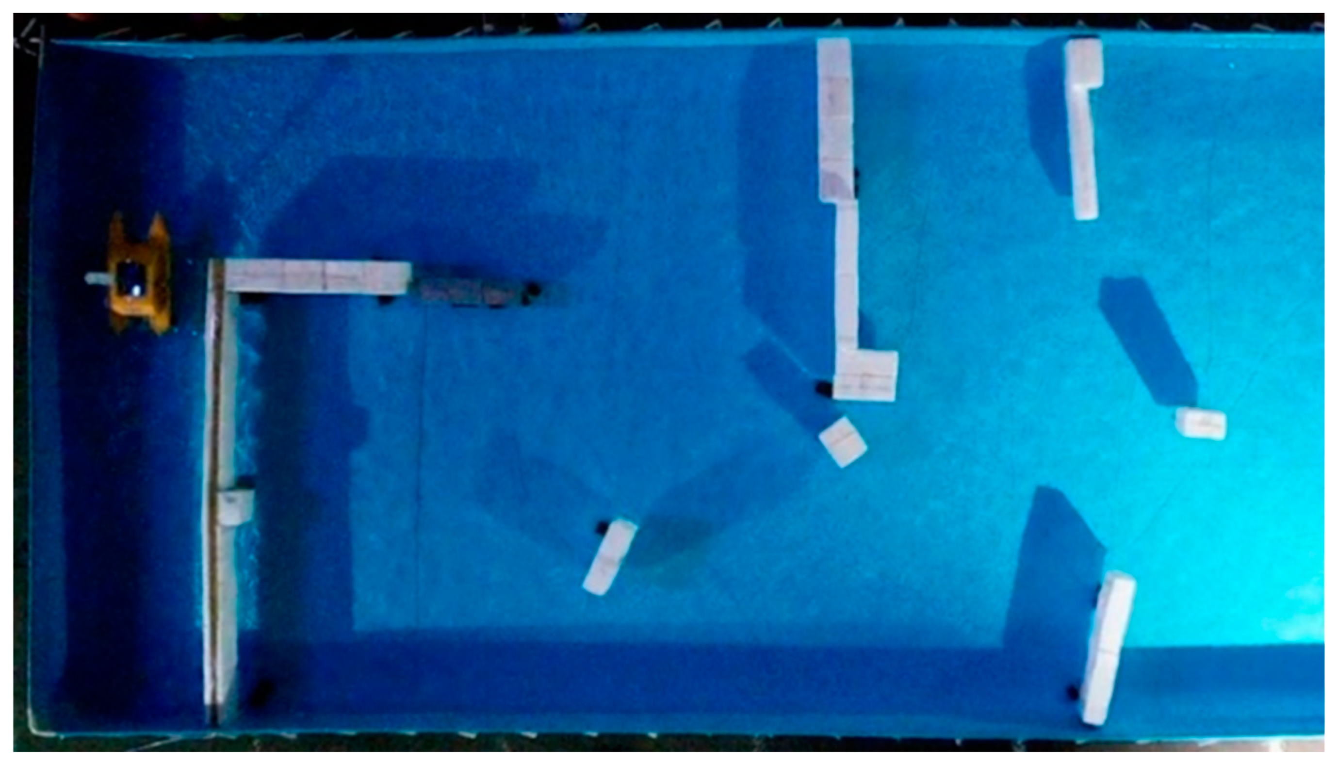
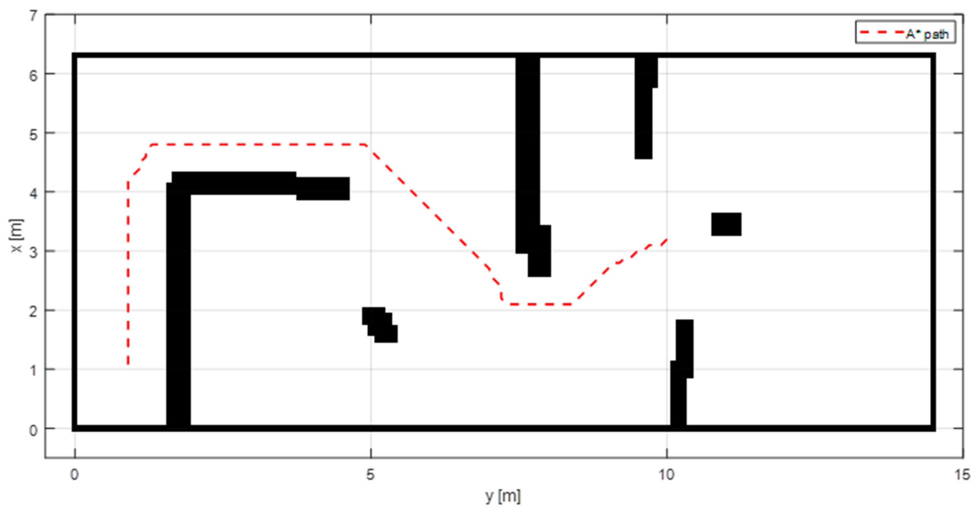
Table 2. Dimensions of the artificial port.
MapDimension
Width14.5 m
Height6.3 m
Start waypoint(0.8, 1)
Goal waypoint(10, 3.2)
Table 3. Analysis results of collision avoidance algorithms.
MethodTime [s]Mean Track Error [m]Mean PWM [-]
APF (1)30.90.47892
APF (2)30.50.48991
APF (average)30.70.48492
Safety zone (1)26.60.62398
Safety zone (2)25.40.584104
Safety zone (average)26.00.603102
CRI (1)24.70.40997
CRI (2)22.90.421108
CRI (average)23.80.415103
Disclaimer/Publisher’s Note: The statements, opinions and data contained in all publications are solely those of the individual author(s) and contributor(s) and not of MDPI and/or the editor(s). MDPI and/or the editor(s) disclaim responsibility for any injury to people or property resulting from any ideas, methods, instructions or products referred to in the content.

