Gradient-Tracking Generalized Vertical Coordinate for Ocean Models: Results of Idealized Experiments Using the Regional Oceanic Modeling System (v3.7)

Abstract

A gradient-tracking generalized vertical coordinate (GT) for ocean models is proposed in the study. The movement of the grid height surfaces is based on a simple Arbitrary Lagrangian–Eulerian (ALE) method ensuring that the discrete representation of the main gradient features of ocean states is uniform and small, optimal for the resolution of gradients in the vertical profile throughout the simulation. We have successfully implemented this algorithm into the Regional Oceanic Modeling System (ROMS v3.7). The numerical experiments used to evaluate the performance of the ALE ROMS include the propagation of linear internal waves, the lock-exchange flow, the gravitational currents over steep topography, and the seamount problem. The results demonstrate that generally, a better solution with significantly less spurious numerical mixing and smaller horizontal pressure gradient force error is produced by the GT coordinate compared to the sigma and s coordinate in ROMS. Further examinations of the GT coordinate are necessary regarding its performance in more realistic scenarios of simulations.

1. Introduction

Ocean models are conventionally built upon the z, sigma, and $\rho$ types of vertical coordinates or a general vertical coordinate that allows for flexible grid placement, e.g., the hybrid one combining z, sigma, and $\rho$ coordinate together. The choice of a specific kind of vertical coordinate reflects the strength (as well as the weakness) of an ocean model built upon it [1,2]. How well the ocean circulation can be numerically solved through a proper design of the vertical coordinates remains an open question for discussion [3,4,5,6].

The characteristics of ocean circulation continuously change in space and time. Whether or not and to what degree the grid height surfaces are implemented to follow these variations is an important issue in the vertical coordinate design [7]. The crossing between the coordinate plane and the density isosurface may lead to excessive numerical mixing. As a result, the water properties in the models can be altered, and the numerical solutions that are sensitive to the tracer distributions become biased. In the z coordinate, the temporal change in grid height surfaces is prohibited. In the z-star [8] or the sigma-type coordinates, the movement of the grid height surfaces is a function of the free-surface elevation. They all belong to one category which is called the Quasi-Eulerian method (QE, e.g., Kasahara [9]) in that the tendency of grid height surfaces is pre-defined. The numerical solution from models based on this method is potentially over-mixing as the alignment between the grid plane and the density isosurface cannot be ensured. In another category of vertical coordinates called the Lagrangian method (LG), such a problem may be avoided because the dia-surface velocities have been precisely canceled out by the grid height surface movement. The isopycnal model is a typical one of this kind [10]. However, the applications of ocean models based on this method are also limited, particularly in the regions of vertically well mixing. Lastly, the Arbitrary Lagrangian–Eulerian method (ALE), which is also a generic form of the QE and LG methods, offers a flexible framework for free vertical grid movements [11]. With a careful design of the ALE algorithm, promising results with a minimum grid effect on diapycnal mixing may be obtained for various cases ranging from the simulations of small-scale internal waves to global ocean circulation [12,13,14,15].

The resolution of the bottom boundary layer in regions of abrupt bathymetric change, e.g., the shelf break, is another critical issue commonly seen for the vertical coordinate design. An inadequate resolution of the motions in the vertical direction may lead to a poor simulation of processes such as the overflows or the gravity-adjusted currents near the bottom. Ocean models built on the z-level coordinate suffer from this problem even though the steplike representation of the sea floor may be ameliorated by the so-called “shaved cell” method [16]. The sigma coordinate is superior in this regard because the grid transformation enables a continuous vertical resolution over steep topography with nonvanishing model layers. However, the resolution of the surface boundary is a different case. The sigma coordinate may be degraded in surface resolution in deep basins since the model layer thickness increases proportionally to the local depth. Conversely, the z coordinate, by fixing the depth of the grid levels not only in shallow water but also in deep ocean, ensures a universal resolution of the air–sea exchange processes. Again, the ocean models built on isopycnal coordinates suffer from a weak stratification in sea surface and shallow water regions. A hybrid coordinate is proposed which combines the merits of z- and sigma coordinates in boundary fitting while reducing the numerical mixing in the interior of the ocean but with added complexities in code implementation.

For vertical coordinates with nonvanishing model layers, the simulations may encounter a severe numerical issue in regions with a steep topography. This problem is well known for terrain-following sigma coordinate models and associated with the computation of the horizontal pressure gradient force (HPGF) in which an error is produced from the correction of the along-grid pressure gradients to be horizontal [17]. The along-grid pressure gradients are large horizontally in regions with a steep topography and vertically near the pycnocline, such that the produced error becomes larger locally and causes unrealistic along-slope currents. To address this issue, several s–z hybrid approaches have been proposed to reduce the error, which essentially is determined by the angle between the sea bottom slope-controlled coordinate plans and isopycnal surfaces. They include the vanishing quasi-sigma-coordinate [18], the σS-z-σB coordinates [19], the generalized piecewise terrain-following coordinate [20], and the multi-envelope s coordinate [21,22].

High-resolution regional/global ocean modeling requires a vertical coordinate that should be smart enough to resolve a wide variety of dynamical processes, such as river plumes, overflows, upwellings, internal waves, eddies, and overturning circulations, across different spatial and temporal scales. Although there is no consensus on which type of coordinate is the best, a rule of thumb is that a hybrid one with the z-like coordinate being specified in the upper ocean, a $\rho$-like coordinate being specified in the interior of the ocean, and a σ-like coordinate being specified over the shallow region and near the bottom should be optimal. One such example of ocean models following this approach is the HYbrid Coordinate Ocean Model (HYCOM), a product of multi-institutional efforts to develop and evaluate a data-assimilative hybrid isopycnal–sigma-pressure (generalized) coordinate ocean model [10]. However, the isopycnal coordinate-based model may still face difficulties in precisely representing the vertical gradients of model variables. In addition, Alistair et al. [23] argued that numerical mixing remained an issue when using HYCOM in high-latitude overflow simulations, indicating a need for more robust vertical coordinate algorithms for global ocean modeling.

One of the key goals for high-resolution regional/global ocean modeling is to resolve the momentum and material exchange processes between the coastal and open oceans. It fundamentally requires a terrain-following-based vertical nonvanishing coordinate such as the s or sigma coordinate, but a more flexible grid placement is needed to overcome the above-mentioned challenges in the simulations. Inspired by the works of Burchard and Beckers [24] and Hofmeister et al. [25], a general vertical coordinate that mimics the hybrid of coordinates for different dynamical regimes is proposed in this study. In addition, an ALE strategy of grid evolution is used which well represents the spatiotemporal variations in model states. The underlying idea is to track the variable’s vertical gradients instead of using the pre-defined density values. The clustering of model grids in areas of steep gradients leads to an improved resolution of the key ocean dynamics and processes. In addition, it resembles the behavior of the isopycnal coordinate to let the coordinate plane follow the density isosurface as closely as possible, thus reducing the error in horizontal pressure gradient computation near the thermocline as well as minimizing the numerical mixing.

Such an approach may also offer significant advantages for wave modeling, particularly in capturing fine-scale vertical dynamics and maintaining numerical stability. While the sigma coordinates provide natural adaptability to free-surface undulations, they often suffer from pressure gradient errors and numerical mixing near steep topographies, which can undermine the accuracy of wave dynamics representation. On the other hand, z coordinates offer simplicity but lack the flexibility required to resolve wave motions in regions with strong vertical gradients. The proposed coordinate addresses these limitations by combining the boundary-refinement strengths of σ coordinates with the ability to track density gradient. This hybrid capability not only enhances the simulation of complex wave processes such as breaking waves, internal waves, and near-bottom interactions but also ensures robust performance across diverse scenarios, from shallow coastal zones to deep ocean basins. These features position the method as a versatile and reliable tool for advancing wave modeling research.

The proposed vertical coordinate has been implemented into ROMS, a typical terrain-following coordinate ocean model commonly used for high-resolution regional simulations. By removing the Eulerian nature of the terrain-following coordinates, the ALE ROMS show promising results in various test cases based on the comparisons with the original ROMS. The main objectives of this study are twofold: (a) introducing the algorithm of the vertical general coordinate with a gradient-tracking ALE method for grid evolution; (b) accessing the numerical performance of the ALE ROMS that is built upon this method based on idealized test experiments.

The remainder of this paper is organized as follows. Section 2 describes the details of the gradient-tracking vertical general coordinate. Section 3 introduces the implementation of the algorithm into ROMS. In Section 4, we use four idealized test experiments to demonstrate that an improved numerical performance can be achieved by the proposed new coordinate. Finally, discussions and summaries are given in Section 5.

2. The Gradient-Tracking Vertical General Coordinate

2.1. Generalized Vertical Coordinate Transformation

The Cartesian coordinate formula of ocean equations needs to be transformed to allow for flexible vertical grid placement. Following Kasahara [9], the rule of the transformation is:

$$t=t^{\ast },x=x^{\ast },y=y^{\ast },r=r(x^{\ast },y^{\ast },z^{\ast },t^{\ast })$$

(1)

where the general vertical coordinate $r$ is defined as a function of the independent variables $x^{*},y^{*},z^{*},$ and $t^{*}$. The Jacobian of the transformation is $J={\partial }_r{z}^{*}={\left({\partial }_{z^{*}}r\right)}^{-1}$, which refers to the layer thickness in discrete form. The definition of $\mathrm{r}$ can be arbitrary, provided that it is monotonic in $\mathrm{z}$ and satisfies total height conservation.

The conventional vertical grids in ocean models such as the $\mathrm{z}$-, sigma-, and $\rho$ coordinate are subsets of the definitions of $r$. For example, the $\mathrm{z}/\rho$ coordinate is specified by using $r=\mathrm{z}/\rho$, while the terrain-following coordinate is specified by using $r=\mathsf{\sigma }=\left(z-\eta \right)/\left(\eta +H\right)$, where $\mathrm{r}$, similar to $\mathsf{\sigma }$, is a scale factor to the local water depth, $\eta$ is the surface elevation, and $H$ is the static depth. However, these methods are not optimal in terms of vertical gradient tracking, because in these ways, the progression of grid height surfaces, that is, the progression of layer thickness, is not free, either remaining static (e.g., $\mathrm{z}$-system), changing analytically with time (e.g., sigma-system), or evolving prognostically (e.g., $\rho$-system). Thus, an ALE strategy of grid evolution is used in the following.

2.2. Gradient-Tracking ALE Method

A simple way to track the grid height surfaces with an optimal resolution of the vertical gradients is proposed. It resembles the grid adaptation strategy developed by Burchard and Beckers (2004, hereafter referred to as BB04) [24] but can be more efficient to implement as the moving of grids toward the solution is not in a time-marching manner. In addition, the application of BB04 to 3D numerical models requires horizontal filtering between adjacent positions of the same grid levels [25]. However, this is not necessary in the present method and makes it easier to use.

Figure 1 illustrates the procedures to implement this method. Here, the vertical profile of function f with an arbitrary shape is divided into $N$ layers (Figure 1a). We chose an initially uniform distribution of the grids for ease of illustration. The $N+1$ positions of the grid height surfaces from the bottom to the sea surface are:

$$-H\left(x,y\right)=z_o\left(x,y\right)<z_1\left(x,y,t\right)<\cdots <z_{N-1}\left(x,y,t\right)<z_N\left(x,y,t\right)=\eta \left(x,y,t\right)$$

(2)

with the variables placed at the center of the layers. Here, $H$ is the bathymetry depth, and η is the surface elevation. As shown in Figure 1a, this grid configuration is not optimal in terms of resolving the vertical gradients. The small feature of variation in the middle of the profile is hardly captured by the grid spacing. Moving the grids along the profile to represent the gradients is required for the grid height surface update.

Hofmeister et al. [25] show that the optimization of the resolution in vertical gradients is equivalent to requiring that the gradients of f in the transformed new coordinate are uniform and small. It is easy to obtain by computing the total variation in the piecewise linear function f that sums up all the differences between adjacent grid levels: $\alpha ={\sum }_{k=0}^N{∆}_{k}f$, where ${∆}_{k}f=ABS(f_{k+1}-f_k)$ for $1\le k\le N-1$. The boundary terms ${∆}_{0}f$ and ${∆}_{N}f$ need to be evaluated approximately. For each model grid height surface, the target value of ${\alpha }_k^{\ast }$ ($0\le k\le N$) that satisfies the optimization is then known, ${\alpha }_k^{\ast }={\alpha }_0-{\displaystyle \frac{k}{N}}\left({\alpha }_0-{\alpha }_N\right)$ (red in Figure 1c,d), which, however, is not equal to the corresponding sequence of ${\alpha }_k$ derived from the grids (blue in Figure 1c,d). Moving the grids toward the solution is determined according to the formula [26]:

$$z_k^{\ast }=z_m+{\displaystyle \frac{\left({\alpha }_k^{\ast }-{\alpha }_m\right)}{\left({\alpha }_m-{\alpha }_{m-1}\right)/\left(z_m-z_{m-1}\right)}}, \mathrm{f}\mathrm{o}\mathrm{r} {\alpha }_m\le {\alpha }_k^{\ast }\le {\alpha }_{m-1}$$

(3)

where $m-1$ and $m$ are the indices of the vertical grids that let the value of ${\alpha }_k^{\ast }$ fall between the range of ${\alpha }_m$ and ${\alpha }_{m-1}$. Note that the computation of ${\alpha }_k^{\ast }$ and ${\alpha }_k$ contains a first-order truncation error which is accumulated in the direction of integration. As shown in Figure 1e,f, the error causes a degradation of the solution toward the end of the grid space. However, this issue can be alleviated effectively by “homogenizing” the errors over the vertical from both the upward and downward evaluation of ${\alpha }_k^{\ast }$ and ${\alpha }_k$. Thus, the final solution for the grid height surface update is shown in Figure 2c. It is optimal in the resolution of the vertical gradients, which otherwise would require a much finer grid of uniform spacing to resolve the small variation in the profile.

We show more examples of grid adaptation in Figure 2 using the profile shapes that are typical in the ocean for variables such as temperature, salinity, and biology (e.g., chlorophyll-a). The gradient tracking method allows fewer grid points to better represent the vertical profiles so that the computational cost of the models may be reduced. In addition, the clustering of grid points in the thermocline resembles the double-sigma-coordinate, which effectively reduces the numerical errors in the baroclinic pressure gradient computation.

2.3. Numerical Treatments

The cumulative summation of the absolute value of the vertical gradients is a necessary step to ensure the monotonicity of the transformed vertical coordinate to z by converting the arbitrary profile into a strictly monotonic increasing one while resembling the original profile’s gradient features. The computation of $\alpha$ requires an approximation of ${∆}_{0}f$ and ${∆}_{N}f$ because the model states are located at the center of the layers, and the differences in f in the surface and bottom half cells cannot be determined directly. However, this is trivial work, as the error in the approximation does not affect the profile’s total variation. Thus, the value of $∆f$ nearest the boundary is used, and we demonstrate that such a simple treatment is numerically stable based on experiments.

The total height conservation of the new vertical coordinate is automatically satisfied after the grid adaptation. At the sea surface, $z_N^{\ast }=z_N=\eta$ because the condition ${\alpha }_N^{\ast }={\alpha }_N$ is applied to Equation (3). Similarly, at the sea bottom, $z_0^{\ast }=z_0=-H$ given that ${\alpha }_0^{\ast }={\alpha }_0$.

The grid adaptation method may be designed to track vertical gradient features from multiple states. It also includes several constraints that are used to improve the resolution in surface and bottom boundaries or relieve the CFL limitation of vertical advection due to an extremely small layer thickness. The details are in the following.

2.3.1. Multiple States

The ocean may consist of a variety of physical and biological processes that are important for accurate model simulations. To precisely follow these variations in the models, an adequate resolution of the vertical gradients for multiple states is necessary. The grid adaptation can still be determined through Equation (3), but the linear sequence of the accumulated variation needs to be evaluated using the formula

$${\alpha }_k={\sum }_{k=0}^{\mathrm{N}}\stackrel{I}{\overbrace{MAX}}\left(\left|{\left({\displaystyle \frac{∆f}{∆R}}\right)}_k^i\right|\right)$$

(4)

where the $i$th state represents either a physical, chemical, or biological variable, $∆R$ is a reference difference in the variable following Hofmeister et al. [25], and the operator $\stackrel{I}{\overbrace{MAX}}$ denotes the maximum value among all the states. It is worth noting that the choice of $∆R$ is subjective and depends on the objective of the model study.

2.3.2. Boundary Refinement

At the ocean surface and bottom boundaries, the vertical grid sizes need to be small to resolve the exchange process of heat, momentum, and/or chemical tracers. However, the regions are generally weak in vertical gradients. The gradient-tracking adaptation method introduced needs to be modified when grid clusterings are required for the surface and bottom regions and at the same time to track gradients in the interior of the oceans.

Here, we use the so-called $\mathrm{s}$ coordinate as a guideline to optimize the near-surface and near-bottom resolution during the grid adaptation. Specifically, a vertical s coordinate $z^s=\mathrm{z}\left({\theta }_s,{\theta }_b,Hc,\eta ,H\right)$ is generated, where ${\theta }_s$ and ${\theta }_b$ are the stretching parameters for the surface and bottom, respectively, and $Hc$ is the critical depth used to maintain surface resolution. The s coordinate ensures the desired grid resolution near both the surface and the bottom. Since this is the optimized solution we want to seek at boundaries, a virtual profile with resolved gradients by the s-grids can be assumed. One of the simplest ways to do that is specifying a difference in the variation between the adjacent $\mathrm{s}$-grid height surfaces as a unit, for example $f_k^s=N-k, \mathrm{f}\mathrm{o}\mathrm{r} k=\mathrm{0,1},2,...,N$, where $f_k^s$ represents the piecewise linear function $f$ in the $\mathrm{s}$-grids. The corresponding values of $f^{sz}$ for the positions of model states are then determined by interpolation from the $\mathrm{s}$-grids, and the accumulation is ${\alpha }_k^s={\sum }_{k=0}^N{∆}_k{f}^{sz}$. In the following, the grid adaptation method described in Equation (3) again can be used to obtain the final solution of $z_k^{\ast }$ but the linear sequence of the accumulated vertical variation has to be the one that combines the gradient features from both the virtual profile of the s-grids and the one including either a single or multiple model states. Specifically, the linear sequence of the accumulated vertical variation is derived from the absolute value of the vertical difference ${\alpha }_k^{sz}$, which is defined as:

$${\alpha }_k^{sz}=\left\{\begin{array}{c}{\alpha }_k^s, for k\le k_{min}^s or k\ge k_{max}^s\\ c_s·{\alpha }_k^z, for k_{max}^s>k>k_{min}^s\end{array}\right.$$

(5)

where ${\alpha }_k^z$ is the value from the model-grid profile, and $k_{max}^s$ and $k_{min}^s$ denote the maximum and minimum index of model levels for the boundary refinement. The coefficient ${\mathrm{c}}_s={\sum }_{k=k_{min}^s+1}^{k_{max}^s-1}{\alpha }_k^s/{\sum }_{k=k_{min}^s+1}^{k_{max}^s-1}{\alpha }_k^z$ is used such that the total variation in ${\alpha }_k^z$ between the $k_{min}^s$ and $k_{max}^s$ levels can be converted into the same amount for ${\alpha }_k^s$, while maintaining the gradient features of the model-grid profile. By setting $0\le k_{min}^s=k_{max}^s\le N$, the original $\mathrm{s}$ coordinate can be resumed. Conversely, to deactivate the boundary refinement option, one can simply choose $k_{max}^s=N,k_{min}^s=0$. In addition, a new set of s coordinates $z^{sGT}=\mathrm{z}\left({\theta }_s^s,{\theta }_b^s,{Hc}^s,\eta ,H\right)$, specifically for boundary refinement, is introduced to distinguish it from the original one.

2.3.3. Isopycnal Tendency

The implementation of boundary refinement can readily be modified to mimic the effect of isopycnal coordinate grid adaptation for a certain density range of the water column if a full isopycnal coordinate in the vertical is known. Again, the linear sequence of the accumulated vertical variation is derived from the absolute value of the vertical difference ${\alpha }_k^{\rho z}$, which is defined as:

$${\alpha }_k^{\rho z}=\left\{\begin{array}{c} {\alpha }_k^z, for k\le k_{min}^{\rho } or k\ge k_{max}^{\rho } \\ c_{\rho }·{\alpha }_k^{\rho }, for k_{max}^{\rho }>k>k_{min}^{\rho } \end{array}\right.$$

(6)

where ${\alpha }_k^{\rho }$ and ${\alpha }_k^z$ are the values from the $\rho$-grid and model-grid profile, respectively, and $k_{max}^{\rho }$ and $k_{min}^{\rho }$ denote the maximum and minimum index of model levels for the isopycnal coordinate grid adaptation. The coefficient ${\mathrm{c}}_{\rho }={\sum }_{k=k_{min}^{\rho }+1}^{k_{max}^{\rho }-1}{\alpha }_k^z/{\sum }_{k=k_{min}^{\rho }+1}^{k_{max}^{\rho }-1}{\alpha }_k^{\rho }$ is used such that the total variation in ${\alpha }_k^{\rho }$ between the $k_{min}^{\rho }$ and $k_{max}^{\rho }$ levels can be converted into the same amount for ${\alpha }_k^z$, while maintaining the gradient features of the $\rho$-grid profile.

2.3.4. Layer Thickness Constraint

The grid adaptation may lead to extremely small layer thicknesses that can easily violate the CFL condition [27] for vertical advection or impose a severe constraint on the model’s time step. Once the $z_k^{\ast }$ is determined using Equation (3), an additional step can be implemented to further adjust the model layer thicknesses with the smallest one no less than a specified value $h_{min}.$ In ascending order, the adjustment is

$$z_k^a=MIN\left(MAX\left(z_{k-1}^{\ast }+h_{min}, z_k^{\ast }\right),z_N^{\ast }-h_{min}\left(N-k\right)\right), for k=\mathrm{1,2},3,...,N-1$$

(7)

Alternatively, in descending order the adjustment is

$$z_k^d=MAX\left(MIN\left(z_{k+1}^{\ast }-h_{min},z_k^{\ast }\right),z_0^{\ast }+h_{min}·k\right), k=N-1,N-2,N-3,...,1$$

(8)

In practice, an average $z_k^{adj}=0.5\ast (z_k^a+z_k^d)$ is calculated to ensure that the adjustment is direction-independent.

Finally, it is common to choose a constant global minimum layer thickness constraint, e.g., 0.5 m, in the models [10]. However, such an approach may incur issues in models with nonvanishing layers, particularly in shallow regions where the vertically average layer thickness is even smaller than the specified value. Here, a spatially and temporally varying constraint is introduced, which equals a fraction of the local average layer thickness. In the formula $h_{min}=c_{adj}{\displaystyle \frac{\left(H+\eta \right)}{N}}$, the fraction coefficient $c_{adj}$ is set to be a typical value of 0.5 and may be subject to change.

2.3.5. Vertical Velocities at the Grid Height Surfaces

The continuity equation is written as

$${\displaystyle \frac{\partial h}{\partial t}}+{\nabla }_h·\left(h\mathbf{u}\right)+{\displaystyle \frac{\partial \dot{r}}{\partial k}}=0$$

(9)

where h is the local layer depth; $\mathbf{u}=〈u,v〉$ are the horizontal velocities; ${\nabla }_h$ is the lateral derivation operator; and $k$ is the vertical unit vector. With grid adaptation, $\dot{r}$ in Equation (9) is the vertical velocity that is relative to the movement of the grid height surface $r^{grid}$. $\dot{r}$ can be derived diagnostically using

$${\dot{r}}_k={\dot{r}}_{k-1}-{\displaystyle \frac{\partial h_k}{\partial t}}-{\nabla }_h·{\left(h\mathbf{u}\right)}_k$$

(10)

once the local layer thickness $h_k$ is updated. The boundary condition of $\dot{r}$ at the ocean bottom is the kinetic velocity $w=-u{\displaystyle \frac{\partial H}{\partial x}}-v{\displaystyle \frac{\partial H}{\partial y}}$, since the $r^{grid}$ is always null.

3. Implementation in ROMS

The gradient-tacking (GT) ALE method for vertical grids was implemented into the Regional Oceanic Modeling System (ROMS v3.7). ROMS is a free-surface primitive-equation ocean model that employs a generally stretched $\mathsf{\sigma }$ coordinate, or s coordinate, in the vertical [28]. The model includes a wide variety of test cases that allow us to thoroughly validate the developed method and make a comprehensive comparison between the $\mathsf{\sigma }$-type and the nonvanishing ALE method of this study in numerical behaviors. The details on the modifications that implement the ALE method into ROMS are described in the Appendix A. The following are the steps to realize the GT coordinate under the framework of ALE.

In brief, grid initialization was conducted at the beginning of the model run such that the significant grid movement that was undesired for the model adjustment to the adaptation could be avoided. Since ROMS uses a split-explicit time-stepping scheme in which the baroclinic mode is advanced after the barotropic mode, the update of vertical grids was performed within the baroclinic loops. Specifically, the grid computation started after the update of the vertically integrated $\mathbf{u}$ and $\eta$, and the procedures of the computation were as follows:

• The linear sequence of the accumulated variation ${\alpha }_k$ was derived from the gradient feature of a single state profile or a profile combining multiple states;
• Boundary refinement or the local isopycnal coordinate was enforced using Equations (5) or (6);
• The target value of ${\alpha }_k^{*}$ ($0\le k\le N$) that optimized the resolution of gradients was generated;
• The grid height surfaces $z_k^{\ast }$ and $z^{n+1}$ were updated according to Equation (3).
• The layer thickness constraint was set to $z^{n+1}$ if necessary.

During grid initialization, the same steps of computation from 1–5 were conducted starting from a uniform sigma grid and initial model states. One may choose to repeat the computation several times to improve the mesh quality after the grid adaptation. In each round of computation, the grids were updated according to the states interpolated from the previous round of calculation.

4. Idealized Test Experiments

The numerical performances of the ALE ROMS were assessed using four idealized test cases including the propagation of linear internal waves, the lock-exchange flow, gravitational currents over steep topography, and a seamount experiment. A linear equation of state was used for all the tests, that is,

$$\rho \left(T,S\right)={\rho }_{ref}\left[1-A\left(T-T_{ref}\right)+B\left(S-S_{ref}\right)\right]$$

(11)

where ${\rho }_{ref}=1028$ kg/m³ is the reference density, $T_{ref}=5$ °C is the reference potential temperature, $S_{ref}=35$ PSU is the reference salinity. The thermal expansion coefficient $\mathrm{A}$ was 2.116 × 10⁻⁴ per °C, and the saline contraction coefficient $\mathrm{B}$ was specified to be zero.

Baroclinic motion in the ocean is directly driven by the pressure gradient force, and this gradient is linked to density, rather than to temperature or salinity alone. In reality, seawater density is a nonlinear function of temperature, salinity, and pressure, typically governed by a set of equations. The dominant factor influencing density variations differs across regions. For instance, in estuarine areas, salinity typically dominates, while in the upper layers of the open ocean, temperature is the main factor. Although the GT coordinate can track temperature and salinity gradients separately, a more suitable approach for realistic simulations is to directly track density. The reason for employing a linear equation of state, rather than a nonlinear one, in this study was to focus on demonstrating the spurious mixing that occurs during tracer advection.

The parameter space for setting up the numerical experiments is listed in

Table 1. Parameters used in idealized experiments that were independent of cases’ settings, where ${\upsilon }_h$ is the horizontal viscosity, ${\nu }_v$ is the vertical viscosity, $k_h$ is the horizontal diffusion, $k_v$ is the vertical diffusion, option LMD indicates the Large, McWilliams, and Doney scheme [29].

	Case 1 Internal Wave	Case 2 Lock Exchange	Case 3 Overflow	Case 4 Seamount
Domain size x, km	250	64	300	500
Domain size y, km	-	-	-	500
Domain size z, m	500	20	4000	4500
Grid cell size, m	5000	500	1500	6200
Time step, s	150	15	10	60
${\nu }_h$$,{\mathrm{m}}^2/\mathrm{s}$	200	200	50	50
${\nu }_v$$,{\mathrm{m}}^2/\mathrm{s}$	LMD	0	0	0
${\kappa }_h$$,{\mathrm{m}}^2/\mathrm{s}$	0	0	0	0
${\kappa }_v$$,{\mathrm{m}}^2/\mathrm{s}$	LMD	0	0	0
$\mathrm{Coriolis},{\mathrm{s}}^{-1}$	-	-	-	1.4405 × 10−4
Run duration	200 d	17 h	24 h	20 d

. To implement the GT coordinate with boundary refinement, the $\mathrm{s}$ coordinate in ROMS was also configured with the selected values of the parameters given in

Table 2. Parameters used in idealized experiments that were dependent on cases’ settings, where $\mathrm{A}\mathrm{D}\mathrm{V}$ is the tracer advection scheme, option $u_1$ indicates the first-order upwind scheme, option $u_3$ indicates the third-order upstream biased scheme, $\mathrm{P}\mathrm{G}\mathrm{R}$ is the horizontal pressure gradient scheme, option $\mathrm{s}\mathrm{t}$ indicates the standard Jacobian scheme presented by Haney [30], option $\mathrm{S}\mathrm{M}$ indicates the scheme presented by Shchepetkin and McWilliams [31], option T indicates temperature, and option - indicates the parameter is not used in this case.

	Case 1 Internal Wave				Case 2 Lock Exchange				Case 3 Overflow					Case 4 Seamount
	${\sigma }_{20}$	${\sigma }_{40}$	${GT}_{20}$	${GT}_{40}$	${\sigma }_{u\mathrm{1,20}}$	${\sigma }_{20}$	${\sigma }_{40}$	$\mathrm{G}\mathrm{T}$	${\sigma }_{20}$	${\sigma }_{40}$	$s_{20}$	$\mathrm{G}\mathrm{T}$	${GT}_s$	${\sigma }_{st}$	${\sigma }_{SM}$	$s_{SM}$	${GT}_{SM}$
$\mathrm{N}$	20	40	20	40	20	20	40	$20$	20	40	$20$	$20$	20	$30$	30	30	30
${\theta }_s$	0	0	-	-	0	0	0	-	0	0	0	-	-	0	0	6	-
${\theta }_b$	0	0	-	-	0	0	0	-	0	0	4	-	-	0	0	0	-
$\mathrm{H}\mathrm{c}$	${10}^{16}$	${10}^{16}$	-	-	${10}^{16}$	${10}^{16}$	${10}^{16}$	-	${10}^{16}$	${10}^{16}$	$50$	-	-	${10}^{16}$	${10}^{16}$	0	-
$\mathrm{A}\mathrm{D}\mathrm{V}$	$u_3$	$u_3$	$u_3$	$u_3$	$u_1$	$u_3$	$u_3$	$u_3$	$u_3$	$u_3$	$u_3$	$u_3$	$u_3$	$u_3$	$u_3$	$u_3$	$u_3$
$\mathrm{P}\mathrm{G}\mathrm{R}$	$\mathrm{S}\mathrm{M}$	$\mathrm{S}\mathrm{M}$	$\mathrm{S}\mathrm{M}$	$\mathrm{S}\mathrm{M}$	$\mathrm{S}\mathrm{M}$	$\mathrm{S}\mathrm{M}$	$\mathrm{S}\mathrm{M}$	$\mathrm{S}\mathrm{M}$	$\mathrm{S}\mathrm{M}$	$\mathrm{S}\mathrm{M}$	$\mathrm{S}\mathrm{M}$	$\mathrm{S}\mathrm{M}$	$\mathrm{S}\mathrm{M}$	$\mathrm{s}\mathrm{t}$	$\mathrm{S}\mathrm{M}$	$\mathrm{S}\mathrm{M}$	$\mathrm{S}\mathrm{M}$
$\mathsf{\alpha }$	-	-	T	T	-	-	-	T	-	-	-	T	T	-	-	-	T
$\mathsf{\Delta }\mathrm{R}$	-	-	1	1	-	-	-	1	-	-	-	1	1	-	-	-	1
$k_{min}^s$	-	-	0	0	-	-	-	0	-	-	-	0	5	-	-	-	0
$k_{max}^s$	-	-	20	40	-	-	-	$20$	-	-	-	$20$	$20$	-	-	-	30
${\theta }_s^s$	-	-	-	-	-	-	-	-	-	-	-	-	0	-	-	-	-
${\theta }_b^s$	-	-	-	-	-	-	-	-	-	-	-	-	4	-	-	-	-
${Hc}^s$	-	-	-	-	-	-	-	-	-	-	-	-	50	-	-	-	-
$c_{adj}$	-	-	0.5	0.5	-	-	-	$0.5$	-	-	-	$0.5$	$0.5$	-	-	-	0.5

. The configuration of GT coordinates for different cases is also given in Table 2. The parameter $c_{adj}$ was set 0.5 throughout all experiments when employing the GT coordinate. Unless otherwise specified, the default third-order upwind scheme for the horizontal tracer advection was implemented in all the idealized experiments.

4.1. Measuring Mixing

The numerical mixing of tracers was taken as a measure of the model performance with the newly developed algorithm. The diagnosis of numerical mixing was based on the variance decay of tracers which, as introduced by Burchard and Rennau [32], is simply calculated as the rate of change between the advected square of the tracer and the square of the advected tracer. That is to say,

$$D^{num}{\left\{{\left(s_j^n\right)}^2\right\}}_i={\displaystyle \frac{{A\left\{{\left(s_j^n\right)}^2\right\}}_i-{\left\{{A\left\{s_j^n\right\}}_i\right\}}^2}{∆t}}$$

(12)

where $A\left\{...\right\}$ is an operator to the square of the tracer ${\left(s_j^n\right)}^2$ and to the tracer itself $s_j^n$ through advection with a numerical stencil $\mathrm{j}$. $∆t$ denotes the time step of the integration.

Following the tracer variance decay approach, the physical mixing can be estimated from the right-hand side terms in the derived equation for the square of the mean tracer ${〈s〉}^2$. It is given in Burchard and Rennau [32] and written as:

$$D^{phys}\left({〈s〉}^2\right)=2K_h{\left({\partial }_x〈s〉\right)}^2+2K_h{\left({\partial }_y〈s〉\right)}^2+2K_v{\left({\partial }_z〈s〉\right)}^2$$

(13)

where $K_h$ is the horizontal tracer diffusivity, and $K_v$ is the vertical tracer diffusivity. In the presently conducted test cases, no horizontal tracer diffusions were specified in the simulations. Thus, Equation (13) was reduced to include only the last term. Moreover, it is worth noting that the diagnosis of numerical mixing using Equation (12) required a strictly monotonic advection scheme. Thus, the first-order upwind scheme was used in the vertical if an evaluation of the numerical mixing was implemented.

4.2. Internal Waves

The propagation of linear internal waves evolved from a temperature perturbation was simulated. The numerical setup of the test case was adopted from the experiments conducted by Petersen et al. [13]. The model domain was a flat-bottom, non-rotating rectangular basin with a depth of $H=500$ m and a horizontal dimension of $L=250$ km. A large horizontal viscosity of 200 m²/s was employed here to suppress the potential grid-scale noise that affects the numerical mixing. The initial temperature distribution consisted of a background stratification,

$$T_0\left(z\right)=T_b+(T_{top}-T_b)\times {\displaystyle \frac{z_{bot}-z}{z_{bot}}}$$

(14)

and the wave-induced temperature perturbation,

$$T\mathrm{\prime }\left(x,z\right)=-A\mathit{cos}\left({\displaystyle \frac{\pi }{2L}}\times \left(x-x_o\right)\right)\mathit{sin}\left(\pi {\displaystyle \frac{\mathrm{z}+∆\mathrm{z}/2}{{\mathrm{z}}_{bot}+∆\mathrm{z}/2}}\right)$$

(15)

where the amplitude of the perturbation $\mathrm{A}$ was 2.0 °C, and $T_{top}=20.1$ °C, $T_{bot}=$ 10.1 °C, $x_o=125$ km, $z_{bot}=-487.5$ m, and $∆z=25$ m. The initial upward lifting of isopycnals at the center of the domain causes both left- and right-propagating internal waves, which rebound at the domain boundaries and then propagate in the opposite direction until meeting the boundaries again. We turned on the vertical tracer mixing using the parameterization option of the Large, McWilliams, and Doney (LMD) [29] in ROMS, enabling us to compare the physical and numerical mixing directly. To test the GT coordinate with different vertical grid sizes, numerical experiments were conducted using 20 (${GT}_{20}$) and 40 (${GT}_{40}$) vertical layers, and the results were compared with the corresponding runs using the sigma-coordinate (${\sigma }_{20}$, ${\sigma }_{40}$).

Figure 3 shows, after 10 days of simulations, the vertical structure of the temperature along the basin. As shown in Figure 3a,b, the simulations with the sigma-coordinate produced a more diffusive vertical profile for both 20 and 40 layers. As a result, the internal wave manifested by the temperature distribution became obscure. In comparison, the simulations with the GT coordinate were much better in terms of resolving the waves and the vertical temperature gradients (Figure 3c,d). In the sigma coordinate, the grid height plane was misaligned with the temperature isosurfaces. However, by following the temperature gradients, the GT coordinate behaved like the isopycnal coordinate and could mimic the waves through the vertical grid movements.

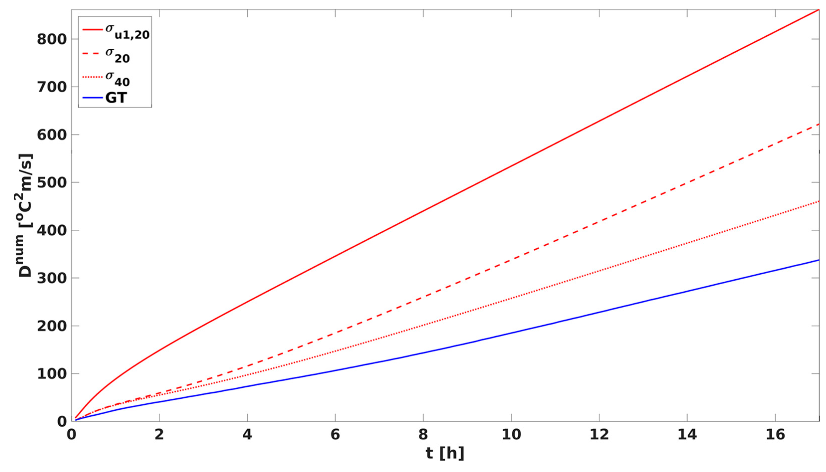
The numerical mixing in the GT coordinate is an order of magnitude smaller than that in the sigma coordinate (Figure 4a). The slow rate of the increase in the GT coordinate is attributed to its capability to follow the temperature gradients and then reduce the vertical fluxes across the grid interfaces. With an increase in the number of model layers from 20 to 40, the numerical mixing is nearly absent in the simulations, exhibiting the typical merit of the isopycnal coordinate. In contrast, the numerical mixing in the sigma coordinate is consistently higher. It is due to the Eulerian nature of the coordinate, so the vertical dia-surface velocities lead to more spurious mixing.

According to Equation (13), the physical mixing is a function of the tracer’s vertical gradients. The smearing-out of the temperature’s vertical gradients by numerical mixing thus weakened the physical mixing in the simulations (Figure 4b). With a smaller amount of numerical mixing in the GT coordinate, the physical mixing incurred by the internal waves was better maintained even after a long integration time.

4.3. Lock-Exchange Flows

The lock-exchange test case is useful for quantifying the effect of numerical mixing on fluid dynamics with a simple model setup. The experiment started with two water masses of different temperatures that were initially at rest and situated side by side in a two-dimensional non-rotating rectangular basin. Here, the simulation employed the following setup for the initial temperature distribution:

$$T\left(x,z,t_0\right)=\left\{\begin{array}{c}5 ℃ \mathrm{for} x<32 \mathrm{km}\\ 30 ℃ \mathrm{for} x\ge 32 \mathrm{km}\end{array}\right.$$

(16)

which has been used by many researchers in previous studies [13,33,34]. For a domain size of $0\le \mathrm{x}\le 64 \mathrm{k}\mathrm{m}$ and a vertical bottom depth $H_o= 20 \mathrm{m}$, a horizontal fine grid resolution $∆x=500$ m was specified. Together with a horizontal momentum viscosity $v_h=200 {\mathrm{m}}^2/\mathrm{s}$, it helped prevent the grid-scale noise from dominating the numerical mixing [33]. We chose the case of the GT coordinate with 20 layers as the control run and compared the result with the simulations using the sigma coordinate but with 20 and 40 vertical layers, respectively. In addition, we compared the result with the simulation under the sigma coordinate and 20 vertical layers but with a horizontal first-order tracer upwind scheme (${\sigma }_{u\mathrm{1,20}}$) to see the effect of horizontal advection on numerical mixing. All simulations were conducted with zero horizontal and vertical tracer diffusion.

The gravitational adjustment occurred immediately at the beginning of the simulations. The dense water intruded into the light water while the latter flowed in the opposite direction on top of the dense water as a result of mass compensation. Without numerical mixing, the exchange process led to a sloping water interface with no intermediate temperatures in between. Figure 5 shows the result of temperature distribution in different tests at the 17th hour. For all the simulations, a certain amount of numerical mixing occurred at the interface. The cases with the sigma coordinate seemed to suffer more from this spurious mixing even though an increase in the vertical resolution could reduce the error significantly. However, a low-order horizontal tracer advection scheme further exacerbated this issue. In comparison, the GT coordinate produced a sharp interface, indicating a small influence from numerical mixing. A notable difference between the results of the sigma and GT coordinates was that in the latter case, the vertical grids were clustered around the interface. This feature allowed the GT coordinate to behave like the isopycnal counterpart, but at the same time, at the head of the gravitational currents where the interface intersects with the surface/bottom boundary, the minimum layer thickness constraint was activated to make sure no outcropping of the grid lines occurred.

The diagnosis of the global numerical mixing supported that its growth in the GT coordinate was relatively slower (Figure 6). Moreover, the tracer variance approach provided a view of where the numerical mixing arose from. As shown in Figure 7, the numerical mixing was mainly along the temperature interface but could be significantly large at the head of the gravitational currents. Away from the head regions, the numerical mixing was larger if the along-grid-line horizontal temperature difference became larger. The GT coordinate was superior to the sigma coordinate because by following the temperature gradients, it significantly reduced the along-grid-line horizontal temperature differences. However, the minimum layer thickness constraint effective at the heads of the currents broke the alignment between the grid planes and temperature isosurfaces. Similar to the cases with the sigma coordinate, they were thus the regions where strong numerical mixing occurred.

The effect of numerical mixing on the exchange flow can be quantitatively compared according to the front propagation speed of the gravitational currents. Benjamin [35] derived a theoretical value of the front velocity,

$$u_f=0.5\sqrt{g{H}_0∆\rho /{\rho }_0}$$

(17)

where $H_0$ is the bottom depth, and $∆\rho$ (0.5438 kg m⁻³ in the study) is the density difference between the two classes of water. The front position can then be determined simply by multiplying the $u_f$ with the model time step.

Table 3. The front positions for different cases (in km). The first row represents the simulation run times (in hours), while the first column lists the case names.

	2 h	6 h	12 h	13 h	15 h	16 h	17 h
${\sigma }_{u\mathrm{1,20}}$	36.5	44	53	55	58	60	61
${\sigma }_{20}$	36	43.5	53	54.5	58	59.5	61
${\sigma }_{40}$	36	43.5	53	55	58	60	61.5
$\mathrm{G}\mathrm{T}$	36	43.5	53	55.5	58.5	60.5	62
theory	36.02	43.07	53.63	55.39	58.91	60.38	62.43

shows comparisons of the front position in all cases against the theoretical prediction. Given that $u_f$ calculated from Equation (17) was 0.4892 m/s, the front advanced linearly and reached 62.4 km at the end of the simulation. In the first 12 h for all cases, the front propagation closely aligned with the theoretical solution, as the specified vertical layer thickness was sufficient for all the simulations to suppress the numerical mixing that may have significantly slowed down the front’s propagation velocity. However, between hours 13 and 17, the cumulative numerical mixing and grid surface distribution led to discrepancies between the front positions of the σ coordinate cases and the theoretical solution. Specifically, at 16 h, the front position in all σ coordinate cases was less than 60 km, whereas the theoretical position was 60.38 km, resulting in a percentage of agreement of 96.1%. In contrast, a better percentage of agreement of over 99.5% could be found in the GT coordinate with only half the number of vertical layers.

4.4. Overflow

In this test, boundary currents in an idealized overflow were simulated. The numerical experiment aimed to validate the GT coordinate with a refinement at the bottom boundary. Following the descriptions in Haidvogel and Beckmann [36], the model domain was two-dimensional, with a horizontal dimension of $0\le \mathrm{x}\le 300 \mathrm{k}\mathrm{m}$. The bottom depth of the slope for the density-driven currents flowing into the ambient ocean was

$$H\left(x\right)=v_1+0.5\left({v_2-v}_1\right)\left(1+tanh\left({\displaystyle \frac{x-x_0}{\psi }}\right)\right)$$

(18)

where ${\mathsf{\nu }}_1=200 \mathrm{m}$, $v_2=4000$ m, $x_0=\mathrm{100,000} \mathrm{m}$, and $\mathsf{\psi }=\mathrm{20,000} \mathrm{m}$. Similar to the lock-exchange case, the overflow was initialized by a temperature distribution with colder water situated on the shelf, that is,

$$T\left(x,z\right)=\left\{\begin{array}{c}0 x\le 42 \mathrm{km}\\ 5 x>42 \mathrm{km}\end{array}\right.$$

(19)

To prevent the grid-scale noise from dominating the numerical mixing, a horizontal grid resolution $∆x=1500$ m and a horizontal momentum viscosity $v_h=50 {\mathrm{m}}^2/\mathrm{s}$ were used. Except for the standard case of a GT coordinate with 20 layers, the same experiment was conducted, but it included a boundary refinement (${\mathrm{G}\mathrm{T}}_s$). For comparison, the experiment using the s coordinate of ROMS ($s_{20}$) was also tested, along with the cases using the sigma coordinate but with 20 and 40 vertical layers, respectively. Again, all the simulations were conducted with zero horizontal and vertical tracer diffusion.

Different from the lock-exchange case, the introduction of a slope caused the intruding dense water on the shelf to be accelerated once entering the slope region. This process continued until the flow exited the slope and reached the flat bottom of the basin where bottom frictions led to a deceleration and a hydraulic jump at the head of the gravitational currents. The result of the temperature distribution from all the tests at the 24th hour when the gravitational currents were away from the slope is shown in Figure 8. The model results varied with the coordinate setups, particularly in terms of frontal locations and the height of the resulting hydraulic jump. Among all cases, the results for ${\sigma }_{20}$ exhibited the weakest front propagation and the highest hydraulic jump, followed by ${GT}_{20}$ in second place and ${\sigma }_{40}$ in third. The cases of $s_{20}$ and $\mathrm{G}\mathrm{T}\mathrm{s}$, however, produced the fastest-moving gravitational currents, which were close in the location and height of the jump. The importance of resolving the bottom boundary in this case was evident as the GT coordinate with the boundary refinement showed a convergent solution toward the s coordinate. The solution of the GT coordinate without the boundary refinement was much worse in comparison and looked like an intermediate value between the solutions of sigma coordinates with 20 and 40 layers, indicating that numerical mixing may not have been the main source of the error.

The global diagnosis of numerical mixing integrated in time before the currents reached 175 km showed that the case of ${GT}_s$ was the best in terms of generating less spurious mixing (Figure 9). It is easy to understand because the resolution of the bottom boundary with a grid refinement significantly reduces the error in predicting the hydraulic jump, and then the temperature feature behind the jump can further be represented by the GT coordinate, so that an optimal is achieved in reducing the numerical mixing.

4.5. Seamount Problem

The GT coordinate is similar to the terrain-following coordinate featuring nonvanishing vertical layers. The model built upon it has the potential to suffer from the horizontal pressure gradient force issue [30,37,38]. The standard seamount problem was selected as the benchmark test through which the magnitude of the error produced by the GT coordinate could be evaluated. Following the model set up in Hofmeister et al. [25], a Gaussian-shaped mountain of 4500 m in height was configured in the middle of a three-dimensional basin with a horizontal length scale of 500 km. The bottom depth of the mountain was defined as

$$H\left(x,y\right)=4500\times \left(1-0.9e^{{\displaystyle \frac{-\left({\left(x-\mathrm{256,000}\right)}^2+{\left(y-\mathrm{256,000}\right)}^2\right)}{{\mathrm{40,000}}^2}}}\right)$$

(20)

The water was initially motionless and horizontally homogenous in the vertical temperature distribution, which was given by

$$T\left(z\right)=5+15e^{min\left(-450,z\right)/1000}$$

(21)

Equation (21) mimicked the temperature profile with a homogenous surface layer by fixing the temperature in the upper 450 m depth of the water column. The profile is representative of the thermocline in the real ocean and such a gradient feature is resolved differently by various vertical coordinates. For the simulations, there was no external forcing, and the explicit tracer mixing was disabled. One can see Table 1 for the details of the model setup. The experiment included three tests for the GT, sigma, and s coordinate, respectively, and used the PGF scheme proposed by Shchepetkin and McWilliams [31] in ROMS (case of ${\sigma }_{SM},s_{SM},{GT}_{SM}$, respectively). In addition, the case that used the sigma coordinate and the standard PGF scheme [37] in ROMS was also tested as a contrast (${\sigma }_{st}$).

Due to the absence of external forcing, the simulations were expected to always yield no motions. However, the horizontal pressure gradient force error would lead to an unrealistic flow around a steep topography. Thus, the domain-averaged kinetic energy and the maximum horizontal velocity were used to quantify the magnitude of the error in the simulations. The domain-averaged kinetic energy is written as

$$E_{kin}={\displaystyle \frac{1}{2V_0}}\left(\sum _{i,j,k}\left(V_{i,j,k}\left(u_{i,j,k}^2+v_{i,j,k}^2\right)\right)\right)$$

(22)

and the maximum horizontal velocity is

$$v_{max}=max\left(u_{i,j,k},v_{i,j,k}\right)$$

(23)

where $V_0$ is the total volume, $V_{i,j,k}$ is the grid cell volume for each cell.

It is necessary to emphasize that the initial temperature profile was represented by the vertical coordinates differently. As demonstrated in Figure 10a,b, the sigma coordinate had a constant layer thickness, which meant the density difference between adjacent vertical layers was large in the thermocline. The s coordinate may have had a slight improvement in terms of reducing the density difference between adjacent vertical layers, although it mainly aimed to increase grid resolution at the surface boundary (Figure 10a,c). The GT coordinate, on the other hand, homogenized the density difference between adjacent vertical layers by changing the layer thickness, so that the grid-resolved gradients in the thermocline were minimal (Figure 10a,d).

The simulation results of $E_{kin}$ and $v_{max}$ from all the tests are shown in Figure 11. The case of ${\sigma }_{st}$ consistently showed the highest $E_{kin}$ and $v_{max}$. The use of the SM PGF scheme significantly improved the model performance, reducing the $E_{kin}$ by one order of magnitude. However, the similarity of numerical performance between the cases of ${\sigma }_{SM}$ and $s_{SM}$ suggested that more vertical layers were needed for further improvement, as the coordinates were not good enough to represent the profile’s gradients well. Notably, $E_{kin}$ in the case of the GT coordinate was further reduced by one order of magnitude, even using the same number of vertical layers. The improvement simply showed how the issue was relieved through a proper design of the vertical grids. It essentially ensured the alignment between the grid planes and density isosurfaces and allowed the clustering of grids around the main gradient feature of the vertical profile, so that the two terms involved in the calculation of the PGF were small and led to a smaller numeric error.

5. Discussion and Conclusions

The numerical simulation of ocean circulation and other dynamic processes relies on horizontal and vertical grid discretizations, which must be highly flexible for constructing accurate numerical solution methods. In the vertical direction, the conventional $\mathrm{z}$, sigma, and $\rho$ types of coordinates have both strengths and weaknesses in representing the ocean dynamics in discrete space and time [39,40,41]. The idea of adaptive vertical coordinates that allow for an arbitrary grid placement and time evolution is thus preferred to fully utilize the merits of conventional coordinates in different dynamic regimes [15,42]. However, the strategy used for adaptation may lead to a highly variable numerical result [24,43,44]. Thus, the proper design of vertical coordinates remains a key issue for numerical ocean modeling of a wide variety of scenarios from regional to global scales [5,6,7].

In this study, an ALE vertical coordinate that aimed to track the main gradient feature of the vertical profile (hereafter referred to as GT) during the simulation was introduced. Although the idea of gradient tracking for vertical grid adaptation has been formally proposed in previous studies [24,25], our strategy to implement the adaptation is different. Specifically, it is based on a simple linear inverse of the grid height surface which is equivalent to the gradients of the target variable in the discrete representation of the vertical profile being uniform. Since the moving of grids toward the solution is not in a time-marching manner and does not require horizontal filtering between adjacent positions of the same grid levels, this algorithm can be implemented much more easily and efficiently.

The numerical performance of the GT coordinate was evaluated in several idealized test cases including the propagation of linear internal waves, the lock-exchange flow, gravitational currents over a steep topography, and the seamount experiment. The criteria for evaluations were based on spurious numerical mixing and the horizontal pressure gradient force error (HPGFE), which are two critical issues in numerical ocean modeling that commonly lead to the degradation of solutions. In the experiment of linear internal wave propagation, the issue of numerical mixing was particularly evident in those models with fixed coordinates, but it could be significantly alleviated if the grids were implemented to move in a Lagrangian manner [13,34]. Although the GT coordinate only involved a vertical movement of the grids, it behaved like the isopycnal coordinate to mimic the wave propagation. Therefore, the numerical mixing in the GT coordinate could be an order of magnitude smaller than that in the sigma coordinate, exhibiting the typical merit of the isopycnal coordinate. The lock-exchange case has been extensively studied by researchers in the context of numerical mixing [13,33,34]. Among the simulations, the numerical mixing was larger if the along-grid-line horizontal temperature difference became larger. The GT coordinate, similar to the isopycnal coordinate, was superior because it could resolve the vertical temperature gradients and cause the alignment between the grid planes and temperature interface between the two water masses, thus significantly reducing the along-grid-line horizontal temperature differences and the numerical mixing. In the overflow experiment, although numerical mixing was not the key issue in the simulations, the GT coordinate with boundary refinement significantly reduced the error in the prediction of the hydraulic jump. In addition, the temperature feature behind the jump could further be represented by the coordinate. Thus, the numerical mixing in that case turned out to be the minimum. Finally, the seamount problem is well known as a benchmark test to examine the HPGFE in ocean models implemented with nonvanishing vertical layers, e.g., the terrain-following coordinate models [20,25,31]. In contrast to the results of sigma and s coordinates using the same number of vertical layers, the domain-averaged kinetic energy produced by the GT coordinate was one order of magnitude smaller. The improvement was achieved because the GT coordinate ensured the alignment between the grid planes and density isosurfaces and at the same time allowed the clustering of grids around the main gradients of the vertical profile, so the two terms involved in the calculation of the PGF were small and led to a smaller numeric error.

The algorithm of the GT coordinate was successfully implemented into ROMS (v3.7). The good performance of the GT coordinate came at the cost of additional computational resources. Specifically, there was an increased computational overhead due to the need to calculate several intermediate variables and perform interpolations to achieve the optimized grid distribution. The overall computational time increased by approximately 7%. However, this additional cost was significantly less than the doubling of the model’s vertical layers (approximately 17% increase in runtime), indicating that the GT coordinate could be efficient and cost-effective. In addition, the implementation of the GT coordinate did not rely on information from horizontally adjacent cells, thus facilitating its applications in models utilizing unstructured grids, such as the Finite Volume Community Ocean Model [45,46]. Further examinations of the GT coordinate are necessary regarding its performance in more realistic scenarios of simulations.