Modeling of Three-Dimensional Ocean Current Based on Ocean Current Big Data for Underwater Vehicles

Abstract

This paper proposes a real-time and high-resolution current system for underwater vehicle simulation and testing based on global ocean current data. The goal was to address the issue of the existing systems for underwater vehicle simulation, whose tests cannot provide real-time and continuous current velocity data. Thus, a three-dimensional ocean current model (3D-OCM) was built for depths of 0~4000 m via the reconstruction of raw current data, fast-access information retrieval, and three-dimensional interpolation. The three interpolation algorithms’ data smoothness and computational times were contrasted. The three-dimensional spline and bilinear algorithm performed the best, taking about 22 milliseconds to acquire the current information anywhere underwater. The comparative analysis revealed that the constructed current system performed strongly in real time and had good velocity data consistency compared with the current data from the National Marine Data Center (NMDC). Furthermore, the running trajectories of the profiling float without interpolation and with three interpolations were contrasted, where the trajectories were more consistent between the three-dimensional spline and bilinear and the three-dimensional Newton and bilinear interpolations. The system can support various marine phenomena for the underwater vehicle’s hardware-in-the-loop (HIL) simulation and testing, and it is meaningful and valuable for increasing the effectiveness of the underwater vehicle’s research and development.

1. Introduction

The ocean current, both on the surface and at mid-depth, has been observed and analyzed for more than half a century [1]; these data are crucial for underwater vehicle studies. Underwater vehicles exhibit nonlinearity and time variation in their motions, making them vulnerable to ocean current influences. The primary factor influencing underwater vehicles is current velocity [2].

Regarding the current velocity’s impact on underwater vehicles, most research was performed on trajectory planning and dynamical performance, which reduces the current to a uniform, regular current field using the nearest neighbor interpolation [3,4,5,6] or taking the current into account as a stream function [7,8]. Moreover, researchers employed a hierarchical modeling strategy to simulate the ocean currents using data from the HYCOM (Hybrid Coordinate Ocean Model) website. However, these were performed using the nearest neighbor interpolation or bilinear interpolation at various depths [9,10,11]. Furthermore, only a few researchers created a continuous current field in a three-dimensional oceanic space using distance-weighted interpolation [12] and JointA 3DUnet network’s three-dimensional interpolation [13].

The demand for real-time computation, continuity, and resolution from an ocean current model is increasing as the accuracy of the underwater vehicle’s model [14,15,16], path planning [17,18,19,20], and position prediction [21,22] improves. Researchers can now create real-time and high-resolution current systems using publicly available current data from websites, such as those for the HYCOM (https://www.hycom.org/) or NMDC (https://mds.nmdis.org.cn/). This study adopted the three-dimensional interpolation method to meet the system’s real-time requirements and combined a lightweight database and geographic information technology to lay a strong foundation for developing an effective, real-time, and high-resolution ocean current system.

This paper proposes a current system based on a lightweight database, geographic information, and three-dimensional mathematical modeling technology utilizing publicly available NMDC current data. The complex current raw data were reconstructed into a simple current data list, which allowed for target data retrieval and current data updates. Furthermore, the 3D-OCM was built by combining spline and bilinear interpolation, which avoided the Longe phenomenon and reduced the computational time. The current system performed strongly in real time and had good velocity data consistency when compared with the National Marine Data Center (NMDC) current data. In this simulation system, the current data for different months can be retrieved and any deployment coordinate can be selected, which supports various marine phenomena when carrying out underwater vehicle HIL simulation and testing. Furthermore, it can provide real-time and continuous current velocity data at any position for underwater vehicles.

2. Methods

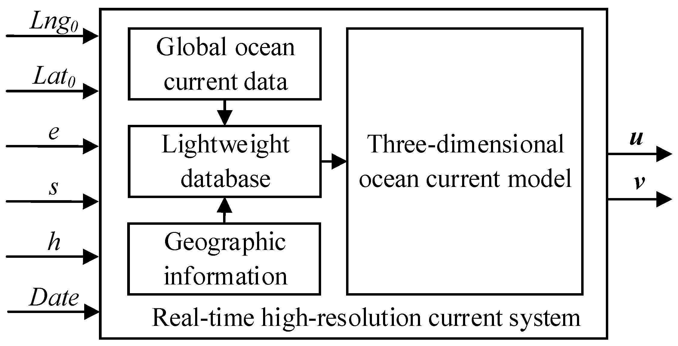
2.1. Real-Time High-Resolution Current System

2.1.1. Current Modeling

Based on global ocean current data and geographic information, the real-time high-resolution current system shown in Figure 1 creates a lightweight current database using current data reconstruction. Next, a 3D-OCM is built by calculating the real-time position and using three-dimensional interpolation. The model can be expressed as follows:

$$[\mathit{u},\mathit{v}]=f_c(Ln{g}_0,La{t}_0,e,s,h,Date)$$

(1)

where u and v are the current velocities along the i- and j-axis, respectively. Lng₀ and Lat₀ represent the longitude and latitude for the underwater vehicle deployment, respectively. e, s, and h are the underwater vehicle positions along the i-, j-, and k-axis, respectively, under the geodetic coordinate system E-ijk. The positive i-, j-, and k-axis are defined as looking eastward, southward, and vertically down, respectively. The date is the month string.

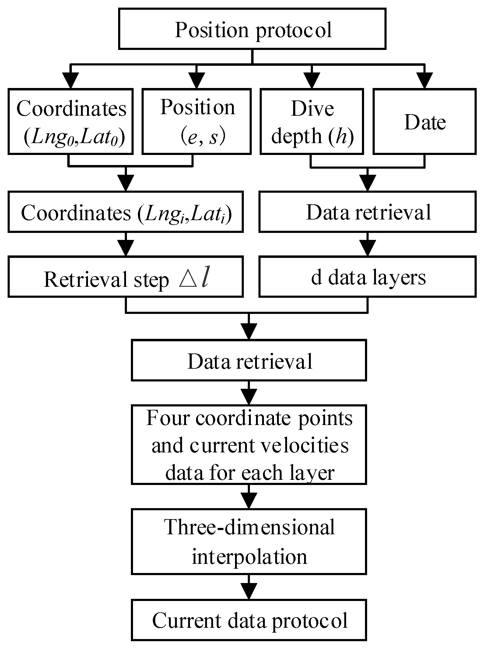
2.1.2. System Workflow

The ocean current system’s workflow is shown in Figure 2. The 3D-OCM takes the deployment coordinates (Lng₀, Lat₀) of the underwater vehicle, its position (e, s, h), and the month as the input parameters. The underwater vehicle first transmits the position protocol to the ocean current system, which obtains the date, dive depth, and deployment coordinates. Then, the real-time coordinates (Lng_i, Lat_i) are obtained through the underwater vehicle’s deployment coordinates and horizontal position, and d data layers are retrieved using the dive depth and date. Additionally, the retrieval range is set in accordance with the real-time coordinate in the ∆l step, and within each data layer, four coordinate, and current velocity data groups are retrieved. Finally, the ocean current system outputs the current data protocol for the underwater vehicle in real time through a three-dimensional global ocean current data interpolation.

2.2. Processing Global Ocean Current Data

2.2.1. Current Data Reconstruction

Current data from January 1958 to December 2022 were acquired from the NMDC website. Multi-grid 3D variational ocean data assimilation was used to process the data, which were derived from the Ocean Reanalysis Product for the Northwest Pacific Ocean Area (CORA V1.0).

The dataset comprised 35 data layers in total, which included longitude data (array size 101 × 1, ranged from 99.5° to 149.5°), latitude data (array size 123 × 1, ranging from −9.5° to 51.5°), velocity u data (array size 101 × 123 × 35), velocity v data (array size 101 × 123 × 35), and depth h data (array size 35 × 1, ranging from 2.5 to 5500 m). The current distribution in the latitude and longitude regions at a 2.5 m underwater depth is shown in Figure 3.

After extracting the date, longitude, latitude, depth, velocity u, and velocity v from the dataset and removing any invalid data, an ocean currents database with around 1.26 × 10⁸ data rows is created. Based on this, SQL queries may be used to retrieve the velocity data using various dates, depths, latitude, and longitude ranges (Figure 4). Furthermore, the latest published current data are updated to the database periodically.

2.2.2. Fast-Access Retrieval of Target Data

The underwater vehicle deployment coordinates are (Lng₀, Lat₀), and the real-time position is (e, s, h). The real-time coordinates (Lng_i, Lat_i) can be solved using Equation (2), and the result is given by Equation (3), where R is the Earth’s average radius, r is the Lat_i radius, and θ is the Lat_i value. Figure 5 shows the underwater vehicle positions.

$$\left\{\begin{array}{l}La{t}_i=La{t}_0+(s/2\pi R)/360\\ Ln{g}_i=Ln{g}_0+(e/2\pi r)/360\\ r=R\cos \theta =R\cos (La{t}_i)\end{array}\right.$$

(2)

$$\left\{\begin{array}{l}La{t}_i=La{t}_0+180\times s/(\pi R)\\ Ln{g}_i=Ln{g}_0+180\times e/(\pi R\cos (La{t}_i))\end{array}\right.$$

(3)

Table 1. The retrieval coefficients.

No	Symbols List	Value
1	The Earth’s average radius R	6,371,393 m
2	The step size of retrieval ∆l	0.5°

shows the retrieval coefficients. The d data layers next to depth h are retrieved based on the underwater vehicle’s position. Then, the underwater vehicle’s real-time coordinates and a step size of ∆l are used to determine the latitude and longitude retrieval ranges. Figure 6 shows the 4 × d group of the coordinates and the current velocity data retrieved from within the longitude range [Lng_i − ∆l, Lng_i + ∆l] and latitude range [Lat_i − ∆l, Lat_i + ∆l] in the total data layers. d is equal to two when using the three-dimensional trilinear interpolation; d is equal to four when using the three-dimensional Newton and bilinear interpolation; and d is equal to n when using the three-dimensional spline and bilinear interpolation, where at this point, depth retrieval is not required.

2.2.3. Current Velocity Position

(Lng_i1, Lat_i1), (Lng_i2, Lat_i1), (Lng_i1, Lat_i2), and (Lng_i2, Lat_i2) are the four neighboring coordinates retrieved by the longitude and latitude ranges at depth h. Based on the underwater vehicle’s position and the retrieved coordinates (Figure 7), the vertical distances d₁, d₂, d₃, and d₄ between the underwater vehicle’s real-time coordinates at depth h and the connecting lines of the four neighboring coordinates are calculated using Vincenty’s formula [23] (Equation (4)). Subsequently, the four coordinate positions under the geodetic coordinate system are obtained as (e₁, s₁, h), (e₂, s₂, h), (e₃, s₃, h), and (e₄, s₄, h) (Equation (5)).

$$\left\{\begin{array}{l}{d}_1=\mathrm{R}*\arccos (\sin (La{t}_{i1})\sin (La{t}_i)+\cos (La{t}_{i1})\cos (La{t}_i)\cos (Ln{g}_i-Ln{g}_i))\\ d_2=\mathrm{R}*\arccos (\sin (La{t}_i)\sin (La{t}_i)+\cos (La{t}_i)\cos (La{t}_i)\cos (Ln{g}_{i1}-Ln{g}_i))\\ d_3=\mathrm{R}*\arccos (\sin (La{t}_{i2})\sin (La{t}_i)+\cos (La{t}_{i2})\cos (La{t}_i)\cos (Ln{g}_i-Ln{g}_i))\\ d_4=\mathrm{R}*\arccos (\sin (La{t}_i)\sin (La{t}_i)+\cos (La{t}_i)\cos (La{t}_i)\cos (Ln{g}_{i2}-Ln{g}_i))\end{array}\right.$$

(4)

$$\left\{\begin{array}{l}(e_1,s_1,h)=(e-d_2,s+d_1,h)\\ (e_2,s_2,h)=(e+d_4,s+d_1,h)\\ (e_3,s_3,h)=(e-d_2,s-d_3,h)\\ (e_4,s_4,h)=(e+d_4,s-d_3,h)\end{array}\right.$$

(5)

2.3. Three-Dimensional Current Modeling

Three-Dimensional Interpolation of the Current Data

• Three-dimensional trilinear interpolation

For the three-dimensional trilinear interpolation, four groups of velocity u and velocity v data in the latitude and longitude region were obtained from the h_m and h_m+1 data layers. First, linear interpolation is carried out along the k-axis to obtain the current data (u_h1, v_h1), (u_h2, v_h2), (u_h3, v_h3), and (u_h4, v_h4) (Figure 8). Second, linear interpolation is carried out along the i-axis to obtain the current data (u_e1, v_e1) and (u_e3, v_e3) (Figure 9). Lastly, linear interpolation is carried out along the j-axis to obtain the current data (u, v) at the underwater vehicle’s position.

Equations (6)–(8) provide the underwater vehicle’s current velocities (u, v) at the real-time position (e, s, h).

Table 2. Three-dimensional trilinear interpolation symbols.

No	Symbols List	Explanation
1	uh1m, uh2m, uh3m, uh4m	Current velocities along the i-axis at depth hm near the real-time position
2	vh1m, vh2m, vh3m, vh4m.	Current velocities along the j-axis at depth hm near the real-time position
3	uh1(m+1), uh2(m+1), uh3(m+1), uh4(m+1)	Current velocities along the i-axis at depth h(m+1) near the real-time position
4	vh1(m+1), vh2(m+1), vh3(m+1), vh4(m+1)	Current velocities along the j-axis at depth h(m+1) near the real-time position
5	uh1, uh2, uh3, uh4	Current velocities along the i-axis at depth h when interpolated along the k-axis
6	vh1, vh2, vh3, vh4	Current velocities along the j-axis at depth h when interpolated along the k-axis
7	ue1, ue2, ue3, ue4	Current velocities along the i-axis at depth h
8	ve1, ve2, ve3, ve4	Current velocities along the j-axis at depth h
9	u	Current velocities at the real-time position
10	v	Current velocities at the real-time position

shows the three-dimensional trilinear interpolation symbols.

$$\left\{\begin{array}{l}{\mathit{u}}_{hi}=(1-t_h){\mathit{u}}_{him}+t_h{\mathit{u}}_{hi(m+1)},i=1,2,3,4\\ {\mathit{u}}_{ej}=(1-t_e){\mathit{u}}_{h(j+1)}+t_e{\mathit{u}}_{hj},j=1,3\\ \mathit{u}=(1-t_s){\mathit{u}}_{ek}+t_s{\mathit{u}}_{e(k+2)},k=1\end{array}\right.$$

(6)

$$\left\{\begin{array}{l}{\mathit{v}}_{hi}=(1-t_h){\mathit{v}}_{him}+t_h{\mathit{v}}_{hi(m+1)},i=1,2,3,4\\ {\mathit{v}}_{ej}=(1-t_e){\mathit{v}}_{h(j+1)}+t_e{\mathit{v}}_{hj},j=1,3\\ \mathit{v}=(1-t_s){\mathit{v}}_{ek}+t_s{\mathit{v}}_{e(k+2)},k=1\end{array}\right.$$

(7)

$$\left\{\begin{array}{l}{t}_h=(h-h_{i(m+1)})/(h_{im}-h_{i(m+1)}),i=1,2,3,4\\ t_e=(e-e_j)/(e_{j+1}-e_j),j=1,3\\ t_s=(s-s_k)/(s_{k+2}-s_k),k=1\end{array}\right.$$

(8)

• Three-dimensional Newton and bilinear interpolation

To reduce the Longe phenomenon impact, four data points are used for Newton interpolation and linear interpolation is carried out for depths less than 10 and more than 3500 m. For the three-dimensional Newton and bilinear interpolation, 16 groups of velocity u and velocity v data in the latitude and longitude regions were obtained from the h_m, h_m+1, h_m+2, and h_m+3 data layers. First, Newton interpolation is carried out along the k-axis to obtain the current data (u_h1, v_h1), (u_h2, v_h2), (u_h3, v_h3), and (u_h4, v_h4) (Figure 10). Second, bilinear interpolation is carried out along the i- and j-axes to obtain the current data (u, v) at the underwater vehicle’s position.

Equations (9) and (10) provide the underwater vehicle’s current velocities (u, v) at the real-time position (e, s, h).

Table 3. Three-dimensional Newton and bilinear interpolation symbols.

No	Symbols List	Explanation
1	uh1m, uh2m, uh3m, uh4m	Current velocities along the i-axis at depth hm near the real-time position
2	vh1m, vh2m, vh3m, vh4m	Current velocities along the j-axis at depth hm near the real-time position
3	uh1(m+1), uh2(m+1), uh3(m+1), uh4(m+1)	Current velocities along the i-axis at depth h(m+1) near the real-time position
4	vh1(m+1), vh2(m+1), vh3(m+1), vh4(m+1)	Current velocities along the j-axis at depth h(m+1) near the real-time position
5	uh1(m+2), uh2(m+2), uh3(m+2), uh4(m+2)	Current velocities along the i-axis at depth h(m+2) near the real-time position
6	vh1(m+2), vh2(m+2), vh3(m+2), vh4(m+2)	Current velocities along the j-axis at depth h(m+2) near the real-time position
7	uh1(m+3), uh2(m+3), uh3(m+3), uh4(m+3)	Current velocities along the i-axis at depth h(m+3) near the real-time position
8	uh1(m+3), uh2(m+3), uh3(m+3), uh4(m+3)	Current velocities along the j-axis at depth h(m+3) near the real-time position
9	uh1, uh2, uh3, uh4	Current velocities along the i-axis at depth h when interpolated along the k-axis
10	vh1, vh2, vh3, vh4	Current velocities along the j-axis at depth h when interpolated along the k-axis
11	ue1, ue2, ue3, ue4	Current velocities along the i-axis at depth h
12	ve1, ve2, ve3, ve4	Current velocities along the j-axis at depth h
13	u	Current velocities at the real-time position
14	v	Current velocities at the real-time position

shows the three-dimensional Newton and bilinear interpolation symbols.

$$\left\{\begin{array}{l}{f}_{\mathit{u}}(h_m,h_{m+1},\cdots ,h_{m+3})={\displaystyle \sum _{j=m}^{m+3}\frac{{\mathit{u}}_{ij}}{{\displaystyle {\prod }_{k=m,j\ne k}^{m+3}(h_j-h_k)}}}\\ {\mathit{u}}_{hi}=f_{\mathit{u}}(h_m)+(h-h_m)f_{\mathit{u}}(h_m,h_{m+1})\\ +\cdots +(h-h_m)(h-h_{m+1})\cdots (h-h_{m+2})\\ f_{\mathit{u}}(h_m,h_{m+1},\cdots ,h_{m+3}),i=1,2,3,4\\ {\mathit{u}}_{ej}=(1-t_e){\mathit{u}}_{h(j+1)}+t_e{\mathit{u}}_{hj},j=1,3\\ \mathit{u}=(1-t_s){\mathit{u}}_{ek}+t_s{\mathit{u}}_{e(k+2)},k=1\end{array}\right.$$

(9)

$$\left\{\begin{array}{l}{f}_{\mathit{v}}(h_m,h_{m+1},\cdots ,h_{m+3})={\displaystyle \sum _{j=m}^{m+3}\frac{{\mathit{v}}_{ij}}{{\displaystyle {\prod }_{k=m,j\ne k}^{m+3}(h_j-h_k)}}}\\ {\mathit{v}}_{hi}=f_{\mathit{v}}(h_m)+(h-h_{m+1})f_{\mathit{v}}(h_m,h_{m+1})\\ +\cdots +(h-h_m)(h-h_{m+1})\cdots (h-h_{m+2})\\ f_{\mathit{v}}(h_m,h_{m+1},\cdots ,h_{m+3}),i=1,2,3,4\\ {\mathit{v}}_{ej}=(1-t_e){\mathit{v}}_{h(j+1)}+t_e{\mathit{v}}_{hj},j=1,3\\ \mathit{v}=(1-t_s){\mathit{v}}_{ek}+t_s{\mathit{v}}_{e(k+2)},k=1\end{array}\right.$$

(10)

• Three-dimensional spline and bilinear interpolation

There is no requirement for retrieval by depth because this interpolation method utilizes 35 data points for spline interpolation from all data layers. For the three-dimensional spline and bilinear interpolation, velocity u and velocity v data in the latitude and longitude regions are obtained from all data layers. First, spline interpolation is carried out along the k-axis to obtain the current data (u_h1, v_h1), (u_h2, v_h2), (u_h3, v_h3), and (u_h4, v_h4) (Figure 11). Second, bilinear interpolation is carried out along the i- and j-axes to obtain the current data (u, v) at the underwater vehicle’s position.

Equations (11)–(14) provide the current velocities (u, v) of the underwater vehicle at the real-time position (e, s, h).

Table 4. Three-dimensional spline and bilinear interpolation symbols.

No	Symbols List	Explanation
1	n	Number of data layers
2	uh11, uh21, uh31, uh41	Current velocities along the i-axis at depth h1
3	vh11, vh21, vh31, vh41	Current velocities along the j-axis at depth h1
4	uh1(m+1), uh2(m+1), uh3(m+1), uh4(m+1)	Current velocities along the i-axis at depth h(m+1) near the real-time position
5	vh1(m+1), vh2(m+1), vh3(m+1), vh4(m+1)	Current velocities along the j-axis at depth h(m+1) near the real-time position
6	uh1(m+2), uh2(m+2), uh3(m+2), uh4(m+2)	Current velocities along the i-axis at depth h(m+2) near the real-time position
7	vh1(m+2), vh2(m+2), vh3(m+2), vh4(m+2)	Current velocities along the j-axis at depth h(m+2) near the real-time position
8	uh1n, uh2n, uh3n, uh4n	Current velocities along the i-axis at depth hn near the real-time position
9	uh1n, uh2n, uh3n, uh4n	Current velocities along the j-axis at depth hn near the real-time position
10	uh1, uh2, uh3, uh4	Current velocities along the i-axis at depth h when interpolated along the k-axis
11	vh1, vh2, vh3, vh4	Current velocities along the j-axis at depth h when interpolated along the k-axis
12	ue1, ue2, ue3, ue4	Current velocities along the i-axis at depth h
13	ve1, ve2, ve3, ve4	Current velocities along the j-axis at depth h
14	u	Current velocities at the real-time position
15	v	Current velocities at the real-time position

shows the three-dimensional spline and bilinear interpolation symbols, spline is the spline interpolation function.

$${\mathit{u}}_{hi}=spline([(h_1,{\mathit{u}}_{hi1}),(h_2,{\mathit{u}}_{hi2}),\dots ,(h_n,{\mathit{u}}_{hin})],h),i=1,2,3,4$$

(11)

$$\left\{\begin{array}{l}{\mathit{u}}_{ej}=(1-t_e){\mathit{u}}_{h(j+1)}+t_e{\mathit{u}}_{hj},j=1,3\\ \mathit{u}=(1-t_s){\mathit{u}}_{ek}+t_s{\mathit{u}}_{e(k+2)},k=1\end{array}\right.$$

(12)

$${\mathit{v}}_{hi}=spline([(h_1,{\mathit{v}}_{hi1}),(h_2,{\mathit{v}}_{hi2}),\dots ,(h_n,{\mathit{v}}_{hin})],h),i=1,2,3,4$$

(13)

$$\left\{\begin{array}{l}{\mathit{v}}_{ej}=(1-t_e){\mathit{v}}_{h(j+1)}+t_e{\mathit{v}}_{hj},j=1,3\\ \mathit{v}=(1-t_s){\mathit{v}}_{ek}+t_s{\mathit{v}}_{e(k+2)},k=1\end{array}\right.$$

(14)

3. Results and Discussion

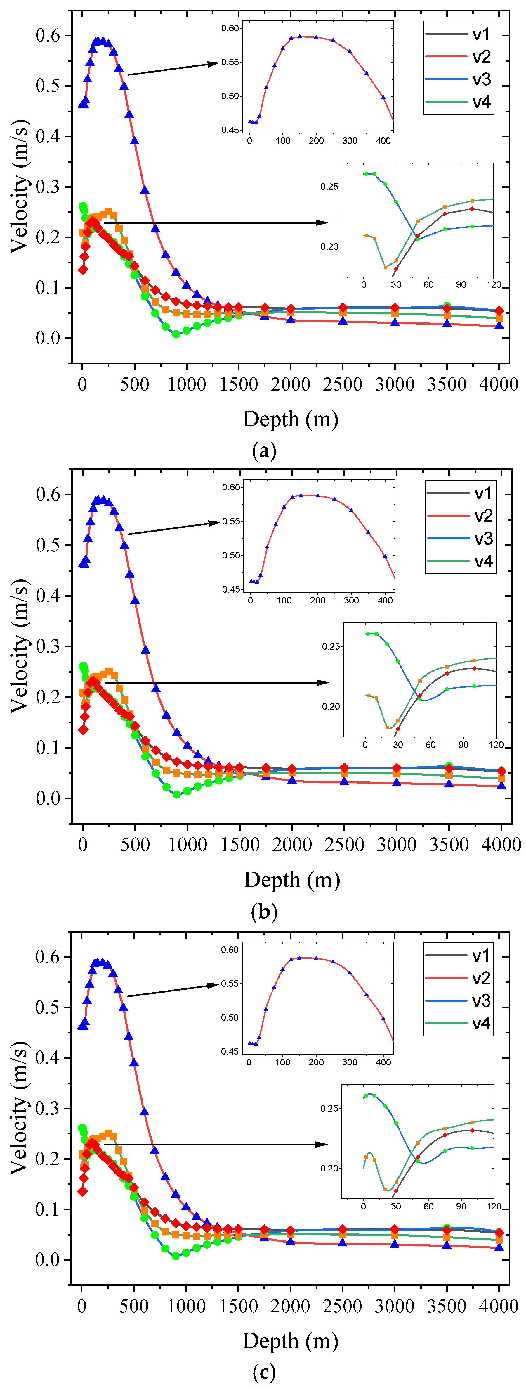
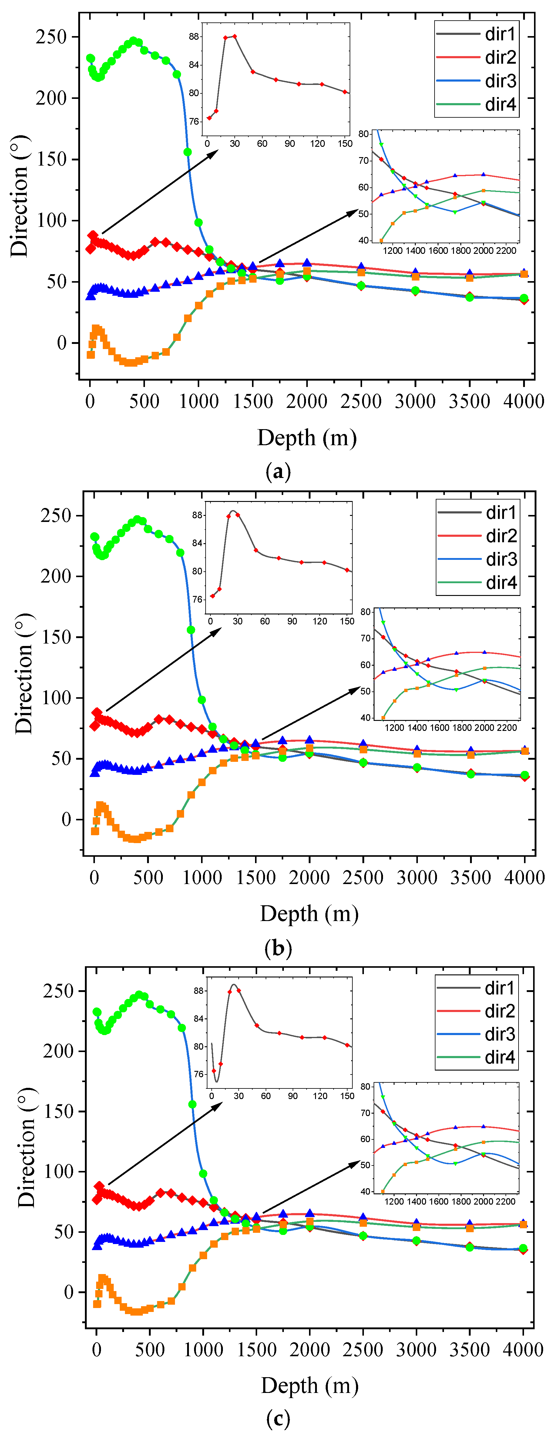
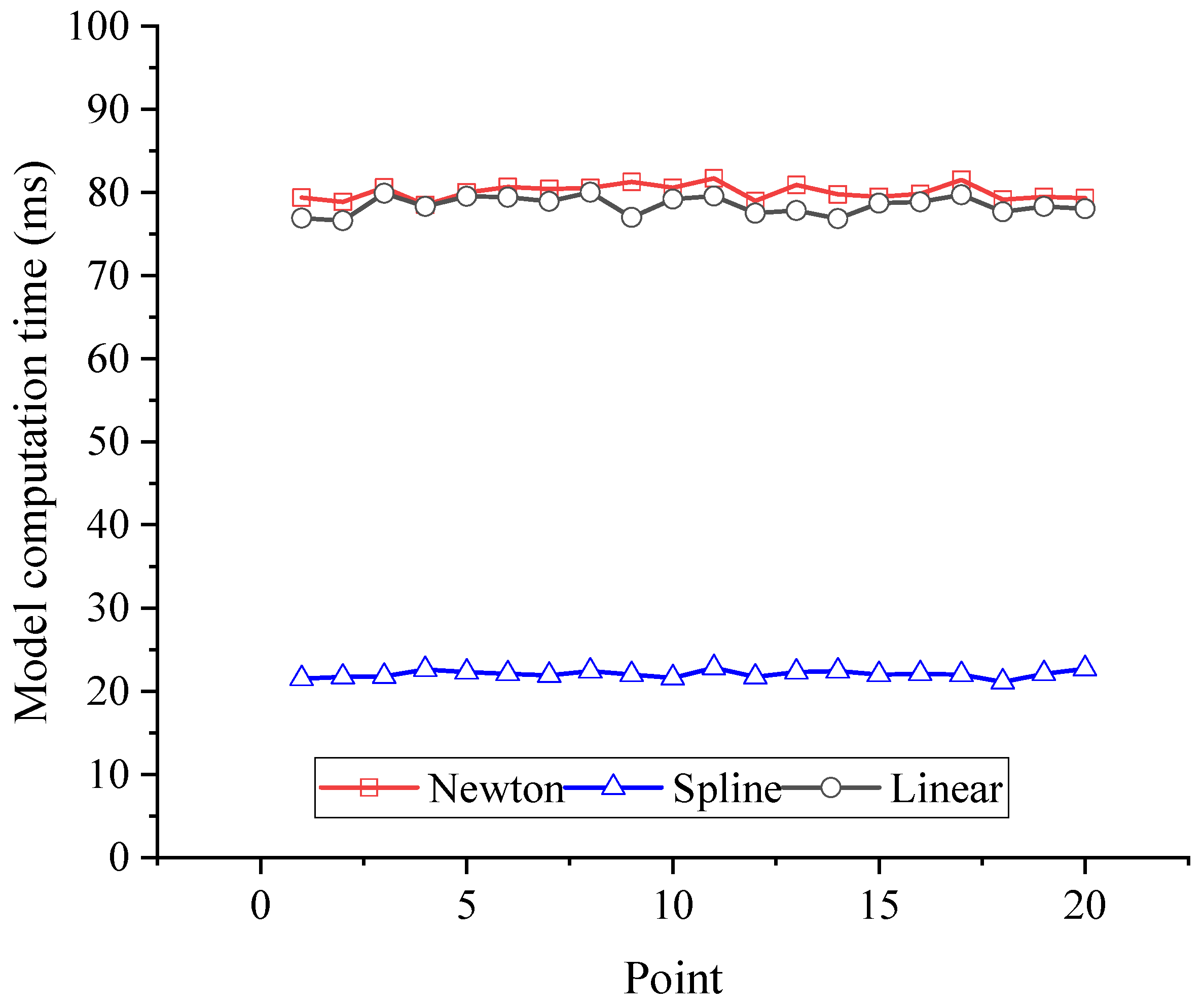
3.1. Effect Comparison of Different Interpolation Methods

The December 2022 current data were selected for analysis, and the coordinates [134.5798° E, 29.7632° N] were chosen as the retrieval location. Figure 12 and Figure 13 show the interpolation curves of the current velocities and directions data at 0~4000 m in the latitude and longitude ranges. The spline interpolation curves were smoother than the linear and Newton interpolation curves for the current velocity and direction. The spline interpolation was also better at capturing changes in the current when they were less than 10 m.

Figure 14 shows the current velocities and directions before the three-dimensional interpolation. Figure 15 and Figure 16 show the three-dimensional spline and bilinear interpolation results, where the retrieved coordinate point was [134.5798° E, 29.7632° N], the depths ranged from 30 to 50 m, the interval was 5 m, and the latitude and longitude resolutions were 0.1° × 0.1° and 0.05° × 0.05°, respectively. The current velocities and directions are represented by the black arrows before the interpolation, and the blue arrows represent the interpolation results.

3.2. Interpolation Results Comparison

All sample points were passed by the curves that resulted from the three interpolation methods along the k-axis. Therefore, the current distribution before and after the three-dimensional interpolation in the sea area east of Luzon Strait at a 2.5 m depth was plotted to verify the interpolation effects along the i- and j-axis. Figure 17 and Figure 18 show that the latitude and longitude resolution after the interpolation was 0.1° × 0.1°. The red markings in Figure 18 show that the NMDC’s current map provided 20 current data.

Figure 19 and Figure 20 show the current velocity and direction error distributions; the absolute direction and velocity errors were all less than 4 × 10⁻³ degrees and 5 × 10⁻³ m/s, respectively.

The current distribution before and after the three-dimensional interpolation in the Japanese warm current sea area at 900 m depth was plotted. Figure 21 and Figure 22 show that the latitude and longitude resolution after the interpolation was 0.1° × 0.1°. The red markings in Figure 22 show that the NMDC’s current map provided 20 current data.

Figure 23 and Figure 24 show that the absolute direction and velocity errors were all less than 5 × 10⁻³ degrees and 5 × 10⁻³ m/s, respectively.

This demonstrates that the constructed current system had good velocity data consistency when compared with the NMDC current data.

Figure 25 and Figure 26 show that the average computational time of the model built using I confirm three-dimensional spline and bilinear interpolation was significantly less than for the three-dimensional trilinear and three-dimensional Newton and bilinear interpolation methods. The results demonstrate that the system could completely satisfy the real-time demands of underwater vehicle’s HIL simulation and testing.

3.3. Property Comparison of Multiple Current Models

Table 5. Multiple current model properties.

No	Current Model	Modeling	High Resolution	Different Currents	Data Authenticity	Data Updatability
1	A stream function	Calculating the function (2D)	√
2	Uniform current field	Nearest-neighbor interpolation (2D)			√
3	3D current field	Bilinear interpolation (2D)			√
4	3D velocity field	3D interpolation	√		√
5	3D-OCM	3D interpolation	√	√	√	√

shows multiple current model properties. The current velocity calculations using a stream function have a high resolution, but it does not imitate actual currents or allow for regular current data updates. A uniform current field is built using the nearest neighbor interpolation for only one depth based on actual currents, but it has poor data smoothing and does not allow for regular current data updates. The three-dimensional current field is built using bilinear interpolation for various depths based on the current raw data obtained from HYCOM. Although it is possible to build a current model from different data, it is not possible to arbitrarily select different currents or allow for regular current data updates, and it has poor data smoothing along the k-axis. The three-dimensional velocity field is built using distance-weighted interpolation and JointA 3DUnet network’s three-dimensional interpolation, but it is not possible to arbitrarily select different current or allow for regular current data updates either. The 3D-OCM was built using three-dimensional spline and bilinear interpolation, which has a high resolution, superior data smoothing in three-dimensional space, and allows for regular current data updates and arbitrarily selecting different currents.

3.4. Profiling Float Trajectories Under the Influence of Currents

A test using the profiling float model was carried out to confirm the present modeling efficacy and the profiling float coefficients (

Table 6. The profiling float coefficients.

No	Symbols List	Value
1	Mass	54.7 kg
2	Surface volume	0.052884 m3
3	Surface density	1025.32 kg/m3
4	Volume at 100 m	0.052734 m3
5	Density at 100 m	1026.66 kg/m3
6	Wetted area	0.77 m2
7	Dive resistance coefficient	0.77
8	Float resistance coefficient	0.46
9	Dive depth	100 m
10	Oil volume change	100 mL

). Figure 27 illustrates the trajectories comparison of the profiling float using the three-dimensional spline and bilinear, three-dimensional Newton and bilinear, and three-dimensional trilinear interpolation methods. The profiling float was only impacted by one current direction at various underwater depths without interpolation, and this clearly differed from the other three interpolated results. Moreover, the float motion exhibited a significant deviation when using three-dimensional trilinear interpolation. In contrast, the profiling float’s trajectory was more consistent when using the three-dimensional Newton and bilinear and three-dimensional spline and bilinear interpolation methods.

4. Conclusions

The real-time high-resolution current system developed in this study was based on a lightweight database, geographic information, and three-dimensional modeling technologies. The 3D-OCM had the quickest computational time when built with three-dimensional spline and bilinear interpolation (around 22 milliseconds) relative to being built using the three-dimensional trilinear, three-dimensional Newton and bilinear, and three-dimensional spline and bilinear interpolation methods. In addition, the running trajectories of the profiling float without interpolation and with the three interpolation methods were contrasted; this showed that the three-dimensional spline and bilinear interpolation was the most advantageous of the three interpolation methods for three-dimensional spatial current data model construction.

The 3D-OCM that was built in this study was very useful and could be easily integrated with other underwater vehicle dynamics models. The model can provide the underwater vehicle with continuous and high-resolution ocean current data at any position from 0 to 4000 m during simulation and testing by importing the deployment coordinates and the underwater vehicle’s position.

The current system had good velocity data consistency when compared with the current data from the NMDC. Furthermore, selecting various dates and deployment coordinates, could support various marine phenomena for the underwater vehicle’s HIL simulation and testing. This has significant practical implications and application value.

Currently, the 3D-OCM can only be built using monthly data. Future studies will collect daily data and investigate the interpolation between different historical dates on which underwater vehicle trajectory predictions were performed.

References

1. Xie, J.; Zhu, J. Estimation of the surface and mid-depth currents from Argo floats in the Pacific and error analysis. J. Mar. Syst. 2008, 73, 61–75. [Google Scholar] [CrossRef]
2. Zhao, D.; Zhang, S.; Gao, S.; Zhong, X. Review on the influence of underwater vehicles motion and load under current. Chin. J. Ship Res. 2024, 19, 1–16. [Google Scholar]
3. Politi, E.; Dimitrakopoulos, G. Comparison of Evolutionary Algorithms for AUVs for Path Planning in Variable Conditions. In Proceedings of the 2019 International Conference on Computational Science and Computational Intelligence (CSCI), Las Vegas, NV, USA, 5–7 December 2019. [Google Scholar]
4. Hu, W. Numerical Simulation of Course-Keeping for Autonomous Underwater Vehicle Under Current Disturbance. Master’s Thesis, Dalian Maritime University, Dalian, China, 2024. [Google Scholar]
5. Men, T.; Wang, Y.; Guan, S.; Ding, J. Research on water outlet location prediction of underwater glider based on ocean current. Ship Sci. Technol. 2023, 45, 66–73. [Google Scholar]
6. Zang, W.; Nie, Y.; Song, D.; Guo, T.; Li, K. Research on Constraining Strategies of Underwater Glider’s Trajectory Under the Influence of Ocean Currents Based on DQN Algorithm OCEANS. In Proceedings of the 2019 MTS/IEEE SEATTLE, Seattle, WA, USA, 27–31 October 2019. [Google Scholar]
7. Alvarez, A.; Caiti, A.; Onken, R. Evolutionary path planning for autonomous underwater vehicles in a variable ocean. IEEE J. Ocean. Eng. 2004, 29, 418–429. [Google Scholar] [CrossRef]
8. Wang, X. Research on Virtual Mooring Control of Underwater Gliders. Master’s Thesis, Tianjin University, Tianjin, China, 2020. [Google Scholar]
9. Lan, W. Research on Underwater Glider Formation Path Planning Under the Influence of Ocean Current. Ph.D. Thesis, Dalian Maritime University, Dalian, China, 2023. [Google Scholar]
10. Ma, Y.; Wang, Y.; Guan, S.; Wang, N.; Ding, J. Motion Control Simulation of Underwater Gliders in Kuroshio. J. Unmanned Undersea Syst. 2024, 32, 1–7. [Google Scholar]
11. Gao, W. Study on path planning of an underwater glider in the complex marine environment. Master’s Thesis, Tianjin University, Tianjin, China, 2022. [Google Scholar]
12. Li, Y.; He, X.; Lu, Z.; Jing, P.; Su, Y. Comprehensive Ocean Information-Enabled AUV Motion Planning Based on Reinforcement Learning. Remote Sens. 2023, 15, 3077. [Google Scholar] [CrossRef]
13. Yao, X.; Cui, M.; Wang, L.; Li, Y.; Zhou, C.; Su, M.; Hu, G. Three-Dimensional Velocity Field Interpolation Based on Attention Mechanism. Appl. Sci. 2023, 13, 13045. [Google Scholar] [CrossRef]
14. Wu, H.; Niu, W.; Wang, S.; Yan, S. A feedback control strategy for improving the motion accuracy of underwater gliders in currents: Performance analysis and parameter optimization. Ocean. Eng. 2022, 252, 111250. [Google Scholar] [CrossRef]
15. Wang, Y.; Zhang, L.; Liang, Y.; Niu, W.; Yang, M.; Yang, S. Modelling and analysis of depth-averaged currents for underwater gliders. Ocean. Eng. 2024, 312, 119086. [Google Scholar] [CrossRef]
16. Jing, G.; Lei, L.; Gang, Y. Dynamic modeling and experimental analysis of an underwater glider in the ocean. Appl. Math. Model. 2022, 108, 392–407. [Google Scholar] [CrossRef]
17. Lan, W.; Jin, X.; Chang, X.; Zhou, H. Based on Deep Reinforcement Learning to path planning in uncertain ocean currents for Underwater Gliders. Ocean. Eng. 2024, 301, 117501. [Google Scholar] [CrossRef]
18. Hu, H.; Zhang, Z.; Li, L.; Peng, X. Energy-optimal motion planning of underwater gliders accounting for seabed Topography and ocean currents. Ocean. Eng. 2023, 288, 116008. [Google Scholar] [CrossRef]
19. Li, X.; Yu, S. Three-dimensional path planning for AUVs in ocean currents environment based on an improved compression factor particle swarm optimization algorithm. Ocean. Eng. 2023, 280, 114610. [Google Scholar] [CrossRef]
20. Lan, W.; Jin, X.; Chang, X.; Wang, T.; Zhou, H.; Tian, W.; Zhou, L. Path planning for underwater gliders in time-varying ocean current using deep reinforcement learning. Ocean. Eng. 2022, 262, 112226. [Google Scholar] [CrossRef]
21. Qiu, B.; Wang, M.; Li, H.; Ma, L.; Li, X.; Zhu, Z.; Zhou, F. Development of hybrid neural network and current forecasting model based dead reckoning method for accurate prediction of underwater glider position. Ocean. Eng. 2023, 285, 115486. [Google Scholar] [CrossRef]
22. Zhang, R.; Wang, Y.; Wan, X.; Ming, Y.; Yang, S. Position prediction of underwater gliders based on a new heterogeneous model ensemble method. Ocean. Eng. 2024, 309, 118312. [Google Scholar] [CrossRef]
23. Zhao, Y.; Lin, L.; Wang, Q.; Wen, P.; Yang, D. Trajectory prediction of sea targets based on geodetic distance similarity calculation. J. Compute. Appl. 2023, 43, 3594–3598. [Google Scholar]
Figure 1. Current model.
Jmse 12 02219 g001
Figure 2. System workflow.
Jmse 12 02219 g002
Figure 3. Currents at 2.5 m water depth.
Jmse 12 02219 g003
Figure 4. Current data reconstruction.
Jmse 12 02219 g004
Figure 5. The underwater vehicle position.
Jmse 12 02219 g005
Figure 6. Target data retrieval schematic.
Jmse 12 02219 g006
Figure 7. Geographic coordinates versus underwater vehicle positions.
Jmse 12 02219 g007
Figure 8. Linear interpolation along the k-axis.
Jmse 12 02219 g008
Figure 9. Linear interpolation along the i- and j-axes.
Jmse 12 02219 g009
Figure 10. Newton interpolation along the k-axis.
Jmse 12 02219 g010
Figure 11. Spline interpolation along the k-axis.
Jmse 12 02219 g011
Figure 12. (a) Linear interpolation along the current velocity k-axis. (b) Newton interpolation along the current velocity k-axis. (c) Spline interpolation along the current velocity k-axis.
Jmse 12 02219 g012
Figure 13. (a) Linear interpolation along the current direction k-axis. (b) Newton interpolation along the current direction k-axis. (c) Spline interpolation along the current direction k-axis.
Jmse 12 02219 g013
Figure 14. Before the three-dimensional spline and bilinear interpolation.
Jmse 12 02219 g014
Figure 15. Three-dimensional spline and bilinear interpolation results (0.1° × 0.1°).
Jmse 12 02219 g015
Figure 16. Three-dimensional spline and bilinear interpolation results (0.05° × 0.05°).
Jmse 12 02219 g016
Figure 17. The 2.5 m water depth east of Luzon Strait (before interpolation).
Jmse 12 02219 g017
Figure 18. The 2.5 m water depth east of Luzon Strait (after interpolation).
Jmse 12 02219 g018
Figure 19. Absolute current velocity errors at 2.5 m depth east of Luzon Strait.
Jmse 12 02219 g019
Figure 20. Absolute current direction errors at 2.5 m depth east of Luzon Strait.
Jmse 12 02219 g020
Figure 21. The Japanese warm current at 900 m depth (before interpolation).
Jmse 12 02219 g021
Figure 22. The Japanese warm current at 900 m depth (after interpolation).
Jmse 12 02219 g022
Figure 23. Absolute current velocity error in the Japanese warm current at 900 m depth.
Jmse 12 02219 g023
Figure 24. Absolute current direction error in the Japanese warm current at 900 m depth.
Jmse 12 02219 g024
Figure 25. Model computation time comparison at 2.5 m depth east of Luzon Strait.
Jmse 12 02219 g025
Figure 26. Computational time comparison for 900 m depth Japanese warm current model.
Jmse 12 02219 g026
Figure 27. (a) Profiling float trajectories comparison before and after interpolation. (b) Profiling float trajectories comparison after interpolation.
Jmse 12 02219 g027