Enhanced Control Strategies for Underactuated AUVs Using Backstepping Integral Sliding Mode Techniques for Ocean Current Challenges

Abstract

This paper examines the control challenges faced by underactuated Autonomous Underwater Vehicles (AUVs) under ocean current disturbances. It proposes a Backstepping Integral Sliding Mode Control (BISMC) strategy to enhance their adaptability and robustness. The BISMC strategy integrates the system decomposition capability of the backstepping control method with the rapid response and robustness advantages of the Sliding Mode Control method, enabling the design of a heading controller and a double closed-loop depth controller. By introducing an integral component, the strategy eliminates steady-state errors caused by ocean currents, accelerating system convergence and improving accuracy. Furthermore, a saturation function is employed to mitigate output chattering issues. Simulation results demonstrate that the BISMC controller significantly enhances the control precision and anti-disturbance capabilities of AUVs under low-frequency ocean current disturbances, showcasing exceptional adaptive and self-disturbance rejection performance.

1. Introduction

Since the dawn of the 21st century, the ocean has emerged as a new frontier for global exploration and development. With advances in marine scientific research, Autonomous Underwater Vehicles (AUVs) have become pivotal in the exploration, development, and study of marine resources, thanks to their remarkable capabilities in autonomous sensing, decision making, and control [1,2]. The degree of autonomy in AUVs is a key metric for assessing their technological progress, while the optimization of motion control systems forms the foundation for achieving high autonomy. However, in the complex and dynamic underwater environment, AUVs face numerous challenges, including strong nonlinear dynamics, internal coupling effects, difficult-to-model dynamic parameters, and unpredictable external disturbances, particularly from random ocean currents. These currents significantly impact heading stability and speed control, increasing the complexity of control strategies. Given the critical importance of energy efficiency for long-distance and prolonged AUV operations, the slender rotating body structure has become the standard in underactuated AUV design due to its efficiency. Nonetheless, this structure’s design—having fewer control degrees of freedom than motion degrees of freedom—places higher demands on control strategy formulation. In real marine environments, disturbances from ocean currents and waves are both common and variable [3,4]. Failing to address these disturbances effectively can severely undermine control performance or even lead to instability in AUV operations. Therefore, exploring robust control strategies with effective disturbance rejection capabilities is crucial for the safe and efficient operation of underactuated AUVs in complex ocean current environments.

Extensive research has been conducted on adaptive and robust control strategies for underactuated AUVs in challenging marine environments, with the development of accurate disturbance models serving as a prerequisite for efficient robust controller design. For instance, Lu Liu et al. developed an output feedback path-following controller that combines an extended state observer with a projection neural network, effectively addressing internal uncertainties and external disturbances [5]. Shen et al. proposed a novel model predictive control framework (LMPC) based on Lyapunov stability, which enhances trajectory tracking accuracy through online optimization techniques and introduces a disturbance observer to estimate comprehensive disturbances [6]. Kim et al. integrated a sliding mode controller with a conventional time-delay controller to improve the position control performance of AUVs in disturbed environments [7]. Notably, much existing research simplifies ocean current disturbances, often treating them as constant or periodically varying disturbance forces. While this simplification captures some influence of ocean currents, it fails to accurately represent their time-varying and unpredictable nature in real environments. To design motion controllers for AUVs that can adapt flexibly to various ocean current conditions, this paper delves into the multidimensional impacts of ocean currents on underactuated AUVs, providing robust technical support to enhance AUV operational efficiency in complex marine settings.

Furthermore, numerous advanced control algorithms have been widely applied in underwater vehicles, including Fuzzy control [8], PID control [9,10], Linear Quadratic Regulator (LQR) [11,12], Backstepping Control (BC) [13], Sliding Mode Control (SMC), Model Predictive Control (MPC) [6,14,15], Adaptive Control [16], and Robust Control [17]. Among these, SMC demonstrates significant potential in addressing the challenges discussed in this paper, owing to its strong anti-disturbance capabilities and adaptability to model uncertainties. However, traditional SMC faces issues of control overshoot and output chattering, necessitating ongoing optimization and refinement. Significant breakthroughs have been achieved in the SMC field. Hangil Joe et al. proposed a second-order SMC for AUVs subject to modeling errors and unknown environmental disturbances, effectively suppressing chattering and improving control accuracy [18]. Konar et al. introduced fractional-order fuzzy SMC, offering a novel solution for depth control in underwater robots, with simulations confirming its excellent transient response and control performance [19]. Haomiao Yu et al. developed a Proportional-Integral-Derivative Sliding Mode Control (PIDSMC) method, enhancing the anti-disturbance capability of SMC and strengthening motion control robustness [20]. Nhut Thanh, Xiaoqiang Dai, Jian Xu, and Jianguo Wu combined the advantages of BC and SMC, proposing backstepping sliding mode control strategies that significantly improve error convergence speed and system stability under uncertainties and unknown disturbances [20,21,22,23,24]. Although convergence speed has greatly improved, instances remain where tracking errors do not converge to zero within a finite time. To address this issue, Lei Qiao et al. proposed two innovative methods: Adaptive Integral Terminal Sliding Mode Control (AITSMC) and Fast Integral Terminal Sliding Mode Control (AFITSMC), which not only accelerate convergence speed but also achieve zero-error convergence within a finite time frame, enhancing the system’s resistance to dynamic uncertainties and time-varying external disturbances [25]. Van et al. designed a controller that combines adaptive neural networks with integral sliding mode, using switching control terms to optimize error approximation while integral terms eliminate steady-state errors, further enhancing system robustness [26].

In summary, recognizing the limitations of existing ocean current disturbance models, which often simplify currents to total disturbance forces, this paper innovatively employs a velocity vector synthesis method, transforming absolute velocity into a relative velocity that incorporates current effects. This approach establishes a more realistic kinematic and dynamic model for AUVs in marine environments. Regarding control strategy, this paper proposes Backstepping Integral Sliding Mode Control (BISMC), integrating the system decomposition benefits of BC with the rapid response and robustness of SMC. By incorporating Dynamic Surface Control (DSC) technology, the “explosion of derivatives” phenomenon is effectively mitigated, optimizing the controller’s transient performance. Additionally, the inclusion of integral terms in the SMC component accelerates convergence and eliminates steady-state errors, enhancing overall robustness. The use of saturation functions in place of traditional switching functions also effectively suppresses control output chattering. To improve depth control accuracy, this paper presents a dual-loop control structure, employing integral sliding mode as the outer loop and BISMC as the inner loop, thereby achieving enhanced control precision.

The remainder of this paper is structured as follows: Section 2 delves into the motion model, rudder force model, and ocean current disturbance model for underactuated AUVs, laying the essential groundwork for the design of efficient control algorithms. Section 3 elaborates on the BISMC method and the design of heading and depth controllers based on it. Additionally, a Lyapunov stability analysis will be conducted to theoretically demonstrate the effectiveness of the proposed control strategy for AUV motion control in complex marine environments. Section 4 will validate the effectiveness and superiority of the proposed method through numerical simulations and comparative experiments. By analyzing experimental results under various operational conditions, the significant advantages of BISMC in enhancing AUV motion control performance will be fully demonstrated. Finally, Section 5 provides a comprehensive summary of this research.

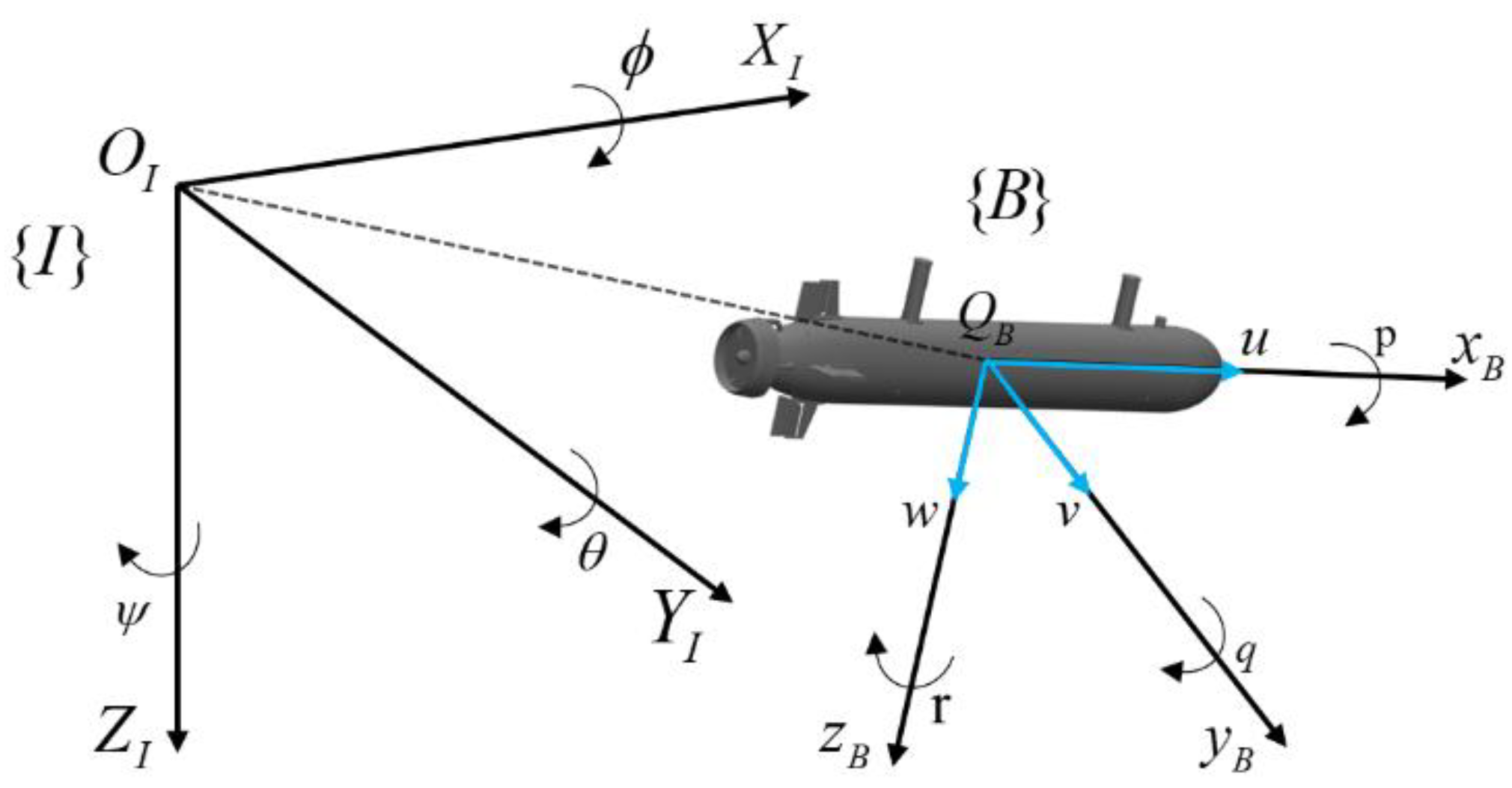
2. Preliminaries and AUV Modeling

2.1. Model Analysis and Simplification

To model the motion and attitude of the AUV while it is underwater, it is common to establish a body-fixed coordinate system, denoted as {B}, and an inertial coordinate system, denoted as {I} (as shown in Figure 1). Euler angles can be utilized to define the angular relationships between the inertial coordinate system and the body-fixed coordinate system of the AUV. These angles also facilitate the description of the AUV’s position and orientation in three-dimensional space. Specifically, the coordinates $(x,y,z)$ of the AUV’s body-fixed coordinate system {B} within the inertial coordinate system {I} are determined by the relative attitude angles $(\varphi ,\theta ,\psi )$ between the two coordinate systems.

The motion model serves as the foundation for underwater robot motion control, ensuring that the controller maintains robust performance even in the face of various uncertainties present in the underwater environment. If the constructed AUV motion model is overly complex, it can complicate the control system, increase the difficulty of controller design, and potentially lead to control system failure. Conversely, if the motion model is too simplistic, it can significantly diminish the performance of the control system and hinder its ability to accurately represent the true motion patterns of AUV [27]. Therefore, it is essential to optimize the spatial motion model of underactuated AUVs effectively. Based on this premise, the following assumptions are made:

Assumption 1. 

The origin of the AUV’s body-fixed coordinate system is established at its center of gravity to facilitate improved analysis and modeling.

Assumption 2. 

The object of study is an underactuated AUV with a cylindrical body that possesses two planes of symmetry: the left–right symmetric  $Q_B{x}_B{z}_B$-plane and the up–down symmetric $Q_B{x}_B{y}_B$-plane.

Assumption 3. 

The AUV is designed with significant static roll stability, such that roll amplitudes in the marine environment are small. Consequently, the roll motion is disregarded in this paper [28].

Based on the above assumptions, referring to relevant papers [29], and using the Newton–Euler equations for rigid bodies and the Lagrangian formulation, we derive the model for a five-degree-of-freedom underactuated AUV:

$$\{\begin{array}{l}\dot{\eta }=J\left(\eta \right)v\hfill \\ M\dot{v}+C\left(v\right)v+D\left(v\right)v+g\left(\eta \right)=d+\tau \hfill \end{array}$$

(1)

In Equation (1), $\eta =[\begin{array}{ccccc}x& y& z& \theta & \psi \end{array}{]}^T$ represents the position and attitude vector of the AUVs, $v=[\begin{array}{ccccc}u& v& w& q& r\end{array}{]}^T$ denotes the velocity vector of the AUV in the body-fixed coordinate system, and $J\left(\eta \right)\in R^{5\times 5}$ is the transformation matrix that converts linear and angular velocities from the body-fixed coordinate system to the inertial coordinate system. $M\in R^{5\times 5}$ is the inertia matrix, which includes the rigid body inertia matrix and added mass. $C\left(v\right)\in {\mathbb{R}}^{5\times 5}$ represents the matrix containing the centripetal and Coriolis forces due to the mass matrix and added mass. $D\left(v\right)\in {\mathbb{R}}^{5\times 5}$ is the damping force and torque matrix due to hydrodynamic effects, and $g\left(\eta \right)\in {\mathbb{R}}^{5\times 1}$ is the restoring force and torque vector. $d={\left[\begin{array}{ccccc}{d}_x& d_y& d_z& d_{\theta }& d_{\psi }\end{array}\right]}^T$ is the environmental disturbance force matrix, and $\tau ={\left[\begin{array}{ccccc}{\tau }_x& 0& 0& {\tau }_q& {\tau }_r\end{array}\right]}^T$ is the control force matrix, where ${\tau }_x$ represents the thrust produced by the propeller, ${\tau }_q$ represents the pitch moment produced by the horizontal rudder angle, and ${\tau }_r$ represents the yaw moment produced by the vertical rudder angle.

2.2. Rudder Force Model

The mathematical model that describes the dynamics of the vertical and horizontal rudders of the underactuated AUV is as follows (The rudder blade structure and rudder mechanism model are shown in Figure 2):

$$\{\begin{array}{l}{\delta }_r={\tau }_r/(2x_N{C}_{LN}\rho A{V}^2)\\ {\delta }_q={\tau }_q/(2x_M{C}_{LM}\rho A{V}^2)\end{array}$$

(2)

$$\dot{\delta }=K_{rud}{\displaystyle \frac{{\delta }_d-\delta }{T_{rud}}}$$

(3)

Here, $x_N$ and $x_M$ are the distances from the rudders to the center of buoyancy; $C_{LN}$ and $C_{LM}$ are the lift coefficients of the rudder blades; $\rho$ is the density of seawater; $A$ is the area of the rudder blade; $V$ is the resultant velocity of the AUV, and $V=\sqrt{u^2+v^2+w^2}$; $K_{rud}$ is the rudder servo control gain; $T_{rud}$ is the time constant of the servo; ${\delta }_d$ is the commanded rudder angle; and ${\delta }_r$ and ${\delta }_q$ are the measured rudder angles.

2.3. Ocean Current Disturbance Model

This paper employs the velocity vector synthesis method to superimpose the disturbances caused by ocean currents on the AUV, converting the absolute velocity into a relative velocity that takes into account the current velocity during the trajectory calculation process. Our approach applies real-time uncertain disturbances to the AUV to simulate the uncertainties of the real marine environment. Let the velocity of the ocean current in the inertial coordinate system be $U_C$, the angle between the projection of the velocity on the $O_I{x}_I{y}_I$ horizontal plane and the $O_I{x}_I$-axis be the horizontal flow direction angle ${\psi }_c$, and the angle between the projection of the velocity on the $O_I{x}_I{z}_I$ vertical plane and the $O_I{x}_I$-axis be the vertical flow direction angle ${\theta }_c$. Then, the velocity of the ocean current in the inertial coordinate system $u_c$, $v_c$ and $w_c$ is expressed as follows:

$$\{\begin{array}{l}{u}_c=U_C\cos ({\theta }_c)\cos ({\psi }_c)\\ v_c=U_C\cos ({\theta }_c)\sin ({\psi }_c)\\ w_c=U_C\sin ({\theta }_c)\end{array}$$

(4)

Through the transformation matrix that converts from the inertial coordinate system to the body-fixed coordinate system, the velocity of the AUV affected by the ocean currents $u_c$, $v_c$ and $w_c$ can be determined.

$$\begin{array}{l}{u}_r=u-(u_c\cos (\psi )\cos (\theta )+v_c\sin (\psi )\cos (\theta )-w_c\sin (\theta ))\\ v_r=v-(-u_c\sin (\psi )+v_c\cos (\psi ))\\ w_r=w-(u_c\cos (\psi )\sin (\theta )+v_c\sin (\psi )\sin (\theta )+w_c\cos (\theta )\end{array}$$

(5)

By substituting Equation (5) into Equation (1), the motion model of the AUV under ocean current disturbance is obtained as:

Kinematic equation:

$$\{\begin{array}{l}\dot{x}=u_r\cos (\psi )\cos (\theta )-v_r\sin (\psi )+w_r\cos (\psi )\sin (\theta )+u_c\\ \dot{y}=u_r\sin (\psi )\cos (\theta )-v_r\cos (\psi )+w_r\sin (\psi )\sin (\theta )+v_c\\ \dot{z}=-u_r\sin (\theta )+w_r\cos (\theta )+w_c\\ \dot{\theta }=q\\ \dot{\psi }=r/\cos (\theta )\end{array}$$

(6)

Dynamic equation:

$$\{\begin{array}{l}(m-X_{\dot{u}})\dot{u}=X_{uu}{u}_r\left|u_r\right|+X_{wq}{w}_{r}q+X_{vr}{v}_{r}r+X_{qq}qq+X_{rr}r\left|r\right|+m(v_{r}r-w_{r}q)+{\tau }_x\\ (m-Y_{\dot{v}})\dot{v}=Y_{rr}r\left|r\right|+Y_{vv}{v}_r\left|v_r\right|+Y_{uv}{u}_r{v}_r+Y_{ur}{u}_{r}r-m{u}_{r}r\\ (m-Z_{\dot{w}})\dot{w}=Z_{uq}{u}_{r}q+Z_{ww}{w}_r\left|w_r\right|+Z_{qq}q\left|q\right|+Z_{uw}{u}_r{w}_r+m{u}_{r}q\\ (I_{zz}-N_{\dot{r}})\dot{r}=N_{vv}{v}_r\left|v_r\right|+N_{uv}{u}_r{v}_r+N_{ur}{u}_{r}r+N_{rr}r\left|r\right|+{\tau }_r\\ (I_{yy}-M_{\dot{q}})\dot{q}=M_{uw}{u}_r{w}_r+M_{qq}q\left|q\right|+M_{ww}{w}_r\left|w_r\right|+M_{uq}{u}_{r}q+Z_{B}B\sin (\theta )+{\tau }_q\end{array}$$

(7)

Here, $X_{**}$, $Y_{**}$, $Z_{**}$, $N_{**}$ and $M_{**}$ represent the various hydrodynamic coefficients of the AUV, $Z_B$ is the distance between the center of buoyancy and the center of gravity, $B$ is the magnitude of the buoyant force, and $I_{zz}$ and $I_{yy}$ are the moments of inertia about the Z and Y axes.

In order to meet the convergence conditions for control in the next section, several reasonable assumptions and lemmas are presented as follows:

Assumption 4. 

The direction angles ${\psi }_c$, ${\theta }_c$ of the ocean current change slowly, and sampling is conducted randomly within the range $[-\pi ,\pi ]$.

Assumption 5. 

The velocity $U_C$ of the ocean current has an upper bound, satisfying $\left|U_C\right|\le {\overline{U}}_C$, $\left|{\dot{U}}_C\right|\le {\overline{\dot{U}}}_C$, where ${\overline{U}}_C$, ${\overline{\dot{U}}}_C$ are positive constants.

Remark 1. 

Due to the continuously changing marine environment and limited energy, the disturbances acting on the AUV can be considered as unknown time-varying but bounded signals with finite rates of change. Therefore, Assumptions 4 and 5 are reasonable.

Remark 2. 

As shown in the dynamics model (7), the AUV discussed in this paper has three linear degrees of freedom. However, since there are no actuators in the sway direction, the number of independent control inputs is two. Therefore, the AUV is a second-order underactuated system.

Remark 3. 

For marine robots, there is inherent actuator saturation [4]. Therefore, the propeller thrust, rudder angle of the vertical fin, and rudder angle of the directional fin for the AUV discussed here should be bounded, i.e., $\left|{\tau }_x\right|\le {\tau }_{x \max }$, $\left|{\tau }_r\right|\le {\tau }_{r\max }$  and $\left|{\tau }_q\right|\le {\tau }_{q\max }$, where ${\tau }_{x \max }$, ${\tau }_{r\max }$  and ${\tau }_{q\max }$ are positive constants.

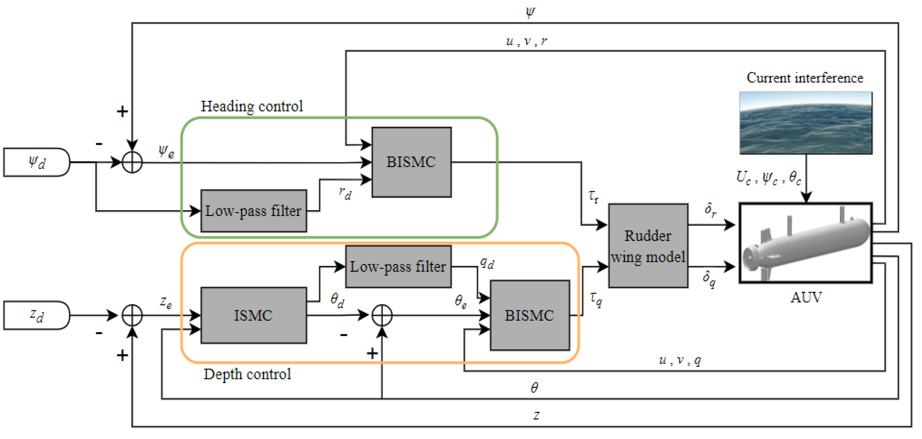
3. Backstepping Integral Sliding Mode Controller Design

To achieve effective motion control, the proposed BISMC controller exhibits strong motion control performance in the presence of ocean currents along with precise and robust control to address high coupling nonlinearity and model uncertainties. The design of this controller integrates backstepping control and sliding mode control methodologies, with enhancements made to improve performance. The control principle block diagram is depicted in Figure 3.

3.1. Heading Controller Design

To simplify the complexity of the controller design, the model for heading control is presented as follows:

$$\{\begin{array}{c}\dot{\psi }=r\\ (I_{zz}-N_{\dot{r}})\dot{r}=N_{vv}v\left|v\right|+N_{uv}uv+N_{ur}ur+N_{rr}r\left|r\right|+{\tau }_r\end{array}$$

(8)

Stabilize the heading error ${\psi }_e$:

$$\{\begin{array}{c}{\psi }_e=\psi -{\psi }_d\\ {\dot{\psi }}_e=r-{\dot{\psi }}_d\end{array}$$

(9)

Define the Lyapunov function:

$$V_1={\displaystyle \frac{1}{2}}{\psi }_e^2$$

(10)

Then,

$${\dot{V}}_1={\psi }_e{\dot{\psi }}_e={\psi }_e(r-{\dot{\psi }}_d)$$

(11)

Define the heading angular velocity error $r_e$:

$$r_e=r-r_d$$

(12)

Then,

$${\dot{V}}_1={\psi }_e(r_e+r_d-{\dot{\psi }}_d)$$

(13)

Define

$$a_1=-k_1{\psi }_e+{\dot{\psi }}_d$$

(14)

where $k_1$ is a strictly positive constant.

In traditional backstepping design, if $r_d=-k_1{\psi }_e+{\dot{\psi }}_d$ is chosen, it may lead to a “differentiation explosion” when computing ${\dot{r}}_d$. By adopting the dynamic surface control method and using a first-order integral filter to calculate the derivative of the virtual control, this drawback can be overcome. Let $r_d$ be the output of the low-pass filter ${\displaystyle \frac{1}{\tau s+1}}$ for $a_1$(as shown in Figure 4):

And $a_1$ satisfies:

$$\{\begin{array}{c}\tau {\dot{r}}_d+r_d=a_1\\ r_d(0)=a_1(0)\end{array}$$

(15)

Here, $\tau$ is a strictly positive constant, and the filtering error generated is $e_1=r_d-a_1$.

The heading control model is classified as a second-order system. The first layer stabilizes the heading angle using backstepping dynamic surface control, while the second layer stabilizes the heading angular velocity through sliding mode variable structure control. To eliminate the steady-state error associated with sliding mode control, an integral of the tracking error is incorporated into the sliding mode surface, resulting in the integral sliding mode surface defined as follows:

$$\{\begin{array}{l}{s}_{\psi }=r_e+c_1{\displaystyle \int r_e}\\ {\dot{s}}_{\psi }={\dot{r}}_e+c_1{r}_e\end{array}$$

(16)

Here, $c_1$ is a strictly positive constant.

Define the Lyapunov function:

$$V_2=V_1+{\displaystyle \frac{1}{2}}{s}_{\psi }^2+{\displaystyle \frac{1}{2}}{e}_1$$

(17)

Then,

$$\begin{array}{cc}\hfill {\dot{V}}_2& ={\dot{V}}_1+s_{\psi }{ s \text{˙}}_{\psi }+e_1{\dot{e}}_1\hfill \\ & ={\psi }_e(r_e+e_1+a_1-{\dot{\psi }}_d)\hfill \\ & +s_{\psi }[(N_{vv}{v}_r\left|v_r\right|+N_{uv}{u}_r{v}_r+N_{ur}{u}_{r}r+N_{rr}r\left|r\right|+{\tau }_r)/(I_{zz}-N_{\dot{r}})-{\dot{a}}_1+c_1{r}_e]+e_1(-{\displaystyle \frac{e_1}{\tau }}+C_1)\hfill \end{array}$$

(18)

where $C_1=c_1{\dot{\psi }}_e-{\ddot{\psi }}_d=c_1(r_e+e_1-c_1{\psi }_e)-{\ddot{\psi }}_d$.

The control law for heading control is designed as:

$$\begin{array}{cc}\hfill {\tau }_r& =(I_{zz}-N_{\dot{r}})[-ET-P{s}_{\psi }-c_1{r}_e-{\psi }_e-(e_1{C}_1)/u+{\dot{a}}_1\hfill \\ & -{\displaystyle \frac{1}{(I_{zz}-N_{\dot{r}})}}(N_{vv}{v}_r\left|v_r\right|+N_{uv}{u}_r{v}_r+N_{ur}{u}_{r}r+N_{rr}r\left|r\right|)]\hfill \end{array}$$

(19)

$$T=\{\begin{array}{l}{\displaystyle \frac{s_{\psi }}{M}},\left|s_{\psi }\right|\le M\\ sign(s_{\psi }),\left|s_{\psi }\right|>M\end{array}$$

(20)

Here, $E$, $P$ and $M$ are strictly positive constants.

Remark 4. 

According to (20), the proposed observer has a saturation function instead of a discontinuous signum function. As a result, unwanted oscillatory effects can be reduced significantly.

3.2. Depth Controller Design

The model for depth control is simplified as follows:

$$\{\begin{array}{c}\begin{array}{l}\dot{z}=-u\theta \\ \dot{\theta }=q\end{array}\\ (I_{yy}-M_{\dot{q}})\dot{q}=M_{uw}uw+M_{qq}q\left|q\right|+M_{ww}w\left|w\right|+M_{uq}uq+Z_{B}B\sin (\theta )+{\tau }_q\end{array}$$

(21)

Depth error formula:

$$\{\begin{array}{c}{z}_e=z-z_d\\ {\dot{z}}_e=-u\theta -{\dot{z}}_d\end{array}$$

(22)

Depth control utilizes a dual-loop control strategy, with the integral sliding mode controller functioning as the outer loop (as shown in Figure 5).

The integral sliding mode surface is defined as follows:

$$\{\begin{array}{l}{s}_z=z_e+c_1{\displaystyle \int z_e}\\ {\dot{s}}_z=-u\theta -{\dot{z}}_d+c_1{z}_e\end{array}$$

(23)

Select the reaching law:

$${\dot{s}}_z=-E_{1}sign(s_z)-P_1{s}_z$$

(24)

Obtain the desired pitch angle ${\theta }_d$ as the virtual control input:

$${\theta }_d=(E_1{T}_1+P_1{s}_z+c_1{z}_e)/u$$

(25)

$$T_1=\{\begin{array}{l}{\displaystyle \frac{s_z}{M_1}},\left|s_z\right|\le M_1\\ sign(s_z),\left|s_z\right|>M_1\end{array}$$

(26)

Here, $E_1$, $P_1$ and $M_1$ are strictly positive constants.

Backstepping integral sliding mode control serves as the outer loop. Define the pitch error formula:

$$\{\begin{array}{c}{\theta }_e=\theta -{\theta }_d\\ {\dot{\theta }}_e=q-{\dot{\theta }}_d\end{array}$$

(27)

The subsequent derivation principle is the same as that for heading control (refer to Equations (8)–(17)), so the specific steps are omitted.

Then, the control law for depth control is designed as:

$$\begin{array}{cc}\hfill {\tau }_q& =(I_{yy}-M_{\dot{q}})[-E_2{T}_2-P_2{s}_{\theta }+{\dot{a}}_2-c_2{q}_e-({\theta }_e{q}_e)/s_{\theta }\hfill \\ & -{\displaystyle \frac{1}{(I_{yy}-M_{\dot{q}})}}(M_{uw}{u}_r{w}_r+M_{qq}q\left|q\right|+M_{ww}{w}_r\left|w_r\right|+M_{uq}{u}_{r}q+Z_{B}B\sin (\theta )]\hfill \end{array}$$

(28)

$$T_2=\{\begin{array}{l}{\displaystyle \frac{s_{\theta }}{M_2}},\left|s_{\theta }\right|\le M_2\\ sign(s_{\theta }),\left|s_{\theta }\right|>M_2\end{array}$$

(29)

Here, $E_2$, $P_2$, $M_2$ are strictly positive constants.

3.3. Lyapunov Stability Verification

This section analyzes the stability of the proposed heading controller algorithm, and the same method can also be used to prove the stability of the depth control.

Theorem 1. 

For Equation (18), there exists a positive constant $Q (Q>0)$ such that $V_2(0)\le Q$, which implies that all signals in the closed-loop system are bounded and converge.

Theorem 2. 

Let $V_2=V_1+{\displaystyle \frac{1}{2}}{s}^2+{\displaystyle \frac{1}{2}}{e}_1=Q$ at this point; then, $C_1$ is bounded, denoted as $D_1$; thus, ${\displaystyle \frac{C_1^2}{D_1^2}}-1\le 0$.

Proof. 

Substituting the control law Equation (18) into the equation for ${\dot{V}}_2$, we obtain:

$$\begin{array}{cc}\hfill {\dot{V}}_2& ={\psi }_e(r_e+e_1)-c_1{\psi }_e^2-k_1\left|s\right|-k_2{s}^2+e_1(-{\displaystyle \frac{e_1}{\tau }}+C_1)\hfill \\ & ={\psi }_e(r_e+e_1)-c_1{\psi }_e^2-k_1\left|s\right|-k_2{c}_2^2{r}_e^2-k_2{c}_2{c}_3{r}_e{\displaystyle \int r_e}-k_2{c}_3^2{({\displaystyle \int r_e})}^2+e_1(-{\displaystyle \frac{e_1}{\tau }}+C_1)\hfill \\ & \le \left|{\psi }_e\right|\left|r_e\right|+\left|{\psi }_e\right|\left|e_1\right|-k_2{c}_2{c}_3\left|r_e\right|\left|{\displaystyle \int r_e}\right|-c_1{\psi }_e^2-k_1\left|s\right|-k_2{c}_2^2{r}_e^2-k_2{c}_3^2{({\displaystyle \int r_e})}^2-{\displaystyle \frac{e_1^2}{\tau }}+\left|e_1{C}_1\right|\hfill \\ & \le {\displaystyle \frac{1}{2}}({\psi }_e^2+r_e^2)+{\displaystyle \frac{1}{2}}({\psi }_e^2+e_1^2)-{\displaystyle \frac{1}{2}}{k}_2{c}_2{c}_3[r_e^2+({\displaystyle \int r_e{)}^2}]-c_1{\psi }_e^2-k_1\left|s\right|-k_2{c}_2^2{r}_e^2-k_2{c}_3^2{({\displaystyle \int r_e})}^2-{\displaystyle \frac{e_1^2}{\tau }}+{\displaystyle \frac{1}{2}}{e}_1^2{C}_1^2+{\displaystyle \frac{1}{2}}\hfill \\ & =(1-c_1){\psi }_e^2+({\displaystyle \frac{1}{2}}-{\displaystyle \frac{1}{2}}{k}_2{c}_2{c}_3)r_e^2+({\displaystyle \frac{1}{2}}+{\displaystyle \frac{1}{2}}{C}_1^2-{\displaystyle \frac{1}{\tau }})e_1^2-k_1\left|s\right|-k_2{c}_2^2{r}_e^2-k_2{c}_3^2{({\displaystyle \int r_e})}^2+{\displaystyle \frac{1}{2}}\hfill \end{array}$$

(30)

There exists a positive constant $h (h>0)$, such that:

$$c_1\ge 1+h,k_2{c}_2{c}_3\ge {\displaystyle \frac{1}{2}}+h,{\displaystyle \frac{1}{\tau }}\ge {\displaystyle \frac{1}{2}}{D}_1+{\displaystyle \frac{1}{2}}+h$$

Then,

$$\begin{array}{cc}\hfill {\dot{V}}_2& \le -h{\psi }_e^2-h{r}_e^2+({\displaystyle \frac{1}{2}}{C}_1-{\displaystyle \frac{1}{2}}{D}_1^2-h)e_1^2-k_1\left|s\right|-k_2{c}_2^2{r}_e^2-k_2{c}_3^2{({\displaystyle \int r_e})}^2+{\displaystyle \frac{1}{2}}\hfill \\ & =-2h{V}_2+({\displaystyle \frac{1}{2}}{C}_1-{\displaystyle \frac{1}{2}}{D}_1^2)e_1^2-k_1\left|s\right|-k_2{c}_2^2{r}_e^2-k_2{c}_3^2{({\displaystyle \int r_e})}^2+{\displaystyle \frac{1}{2}}\hfill \\ & \le -2h{V}_2+{\displaystyle \frac{1}{2}}\hfill \end{array}$$

(31)

Since at this point $V_2=Q$, then Equation (31) can be rewritten as ${\dot{V}}_2\le -2hQ+{\displaystyle \frac{1}{2}}$. To ensure that ${\dot{V}}_2\le 0$, take $-2hQ+{\displaystyle \frac{1}{2}}\le 0$; we can derive that $h\ge {\displaystyle \frac{1}{4p}}$.

Equation (31) shows that when $h\ge {\displaystyle \frac{1}{4p}}$, if $V_2(0)\le p$, then ${\dot{V}}_2\le 0$, and consequently $V_2(t)\le p$.

Furthermore, based on the above reasoning, the following convergence analysis can be performed. According to Inequality Lemma [30], the solution to the inequality equation ${\dot{V}}_2\le -2h{V}_2+{\displaystyle \frac{1}{2}}$ is:

$$V(t)⩽e^{-2h(t-t_0)}V(t_0)+{\displaystyle \frac{e^{-2ht}}{2}}{\int }_{t_0}^t{e}^{{\eta }_1\tau }d\tau =e^{-2h(t-t_0)}V(t_0)+{\displaystyle \frac{1}{4h}}(1-e^{-2h(t-t_0)})$$

(32)

Then,

$$\underset{t\to \infty }{\lim }V(t)⩽{\displaystyle \frac{1}{4h}}$$

(33)

Thus, $V(t)$ converges asymptotically, with the convergence accuracy depending on $h$.

Furthermore, since ${\displaystyle \frac{1}{\tau }}\ge {\displaystyle \frac{1}{2}}{C}_1+{\displaystyle \frac{1}{2}}+h$, if $\tau \to 0$ is taken, then $h\to +\infty$ can be taken, which is the reason why the low-pass filter can be designed as ${\displaystyle \frac{1}{\tau s+1}}$. □

4. Simulation Verification

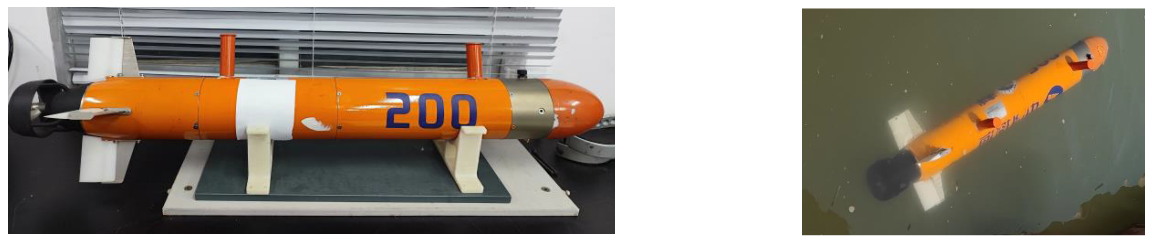
4.1. Parameters of the Underactuated AUV

To verify the effectiveness and robustness of the proposed motion controller, a simulation environment was developed using MATLAB R2022b software (MathWorks, Inc., Natick, United States). The simulation model of the underactuated AUV is based on physical data (as shown in

Table 1. AUV parameter list in the simulations.

Parameter	Value	Parameter	Value
$\rho$	1000 (kg/m3)	$Y_{uv}$	−21.01
$m$	11 (kg)	$Y_{ur}$	3.834
$L$	1.2 (m)	$Z_{\dot{w}}$	−26.08
$W$	106.0 (N)	$Z_{ww}$	−96.22
$B$	107.9 (N)	$Z_{qq}$	−41.9
$l_{xx}$	0.016 (kg · m2)	$Z_{uw}$	−21.01
$l_{yy}$	0.8 (kg · m2)	$Z_{uq}$	−3.834
$l_{zz}$	0.8 (kg · m2)	$M_{\dot{q}}$	−2.918
$Z_B$	0.0296	$M_{qq}$	−112.4
$X_{\dot{u}}$	−0.683	$M_{ww}$	2.107
$X_{uu}$	−1.428	$M_{uw}$	1.591
$X_{wq}$	−26.08	$M_{uq}$	−1.325
$X_{qq}$	−1.279	$N_{\dot{r}}$	−2.918
$X_{vr}$	−26.08	$N_{rr}$	−56.21
$X_{rr}$	−1.279	$N_{vv}$	−2.107
$Y_{\dot{v}}$	−26.08	$N_{uv}$	−1.591
$Y_{vv}$	−96.22	$N_{ur}$	−1.325
$Y_{rr}$	−0.419

) from the “Sprite 200”(as shown in Figure 6) robot in the author’s laboratory, with the controller parameters provided in

Table 2. Heading controller parameters.

BC		SMC		BISMC
Parameter	Value	Parameter	Value	Parameter	Value
k1	2	c1	1	k1	2
k2	10	E	6	τ	0.025
		P	2	c1	0.5
				E	6
				P	2
				M	5

and

Table 3. Depth controller parameters.

BC		SMC		ISMC		BISMC
Parameter	Value	Parameter	Value	Parameter	Value	Parameter	Value
k1	1.5	c1	2	c1	1	k1	1.5
k2	6	c2	4	E1	10	τ	0.025
k3	2	E	10	P1	3	c2	0.5
		P	3	M1	5	E2	10
						P2	3
						M2	5

.

This paper presents a comprehensive evaluation of BISMC through four simulation experiments. Case 1 validates fundamental functionality under ideal conditions. Case 2 testes robustness against static disturbances, while Case 3 assesses adaptability in dynamic environments. Case 4 poses the ultimate challenge with random disturbances, mirroring real oceanic conditions.

Additionally, to analyze the AUV motion control performance more clearly and quantitatively, data analysis was conducted on the heading and depth errors. Four key performance indicators are as follows: (1) IAE (Integral of Absolute Error), expressed as $IAE={\displaystyle {\int }_0^t}\left|e(t)\right|dt$; (2) AVE (Average Value of the Absolute Errors), expressed as $AVE=(1/t){\displaystyle {\int }_0^t}\left|e(t)\right|dt$; (3) ITAE (Integrated Time Absolute Error), expressed as $ITAE={\displaystyle {\int }_0^t}t\left|e(t)\right|dt$; and (4) ASSE (Average Steady State Error), expressed as $ASSE=(1/t){\displaystyle {\int }_0^t}\left|e(t)\right|dt$, where $t$ represents the time after the error converges and stabilizes. In consideration of the impact of ocean current disturbances that arise after the first expected value in the course of heading tracking, we select data subsequent to this first expected value for subsequent calculation and analysis to ensure the accuracy of statistical data.

4.2. Simulation Model Validation

In order to ensure the accuracy, reliability, and practicality of the simulation model, an underactuated AUV entity turning test was conducted on the Shazhou Jinhu Lake in Zhangjiagang Chain(as shown in Figure 7). The trajectory of the AUV was exported from the mounted Doppler sensor. During the test, the wind speed was around 1.5 m/s, and the wind direction was westerly.

Figure 8 presents a comparison of the turning rates between the physical model and the simulation under different rudder angles. It is evident that the two are similar and correspond well with each other. Based on this result, we can conclude that the simulation model we have constructed is effective and reliable, and can be utilized for further analysis and research.

4.3. Case Results

The AUV follows headings of [0°, 20°, 40°, 10°] at 30 s intervals and depths of [0 m, −10 m, −30 m, −20 m] at 50 s intervals. The initial position and velocity of the AUV are both set at ${[x y z \psi \theta ]}^T={[0 0 0 0 0]}^T$, ${[u v w r q]}^T={[0 0 0 0 0]}^T$. The propeller speed was set to 1200 RPM, and the longitudinal speed stabilized at 2.5 m/s after reaching equilibrium. The disturbance of ocean currents in the simulation is introduced into the motion model after the first expected value of AUV tracking. The settings of ocean currents in Cases 2, 3, and 4 are as follows (The ocean current speed for Case 4 is shown in Figure 9):

Case 2:

$$\{\begin{array}{l}{U}_c=0.3 \mathrm{m}/\mathrm{s}\\ {\psi }_c=45°\\ {\theta }_c=45°\end{array}$$

Case 3:

$$\{\begin{array}{l}{U}_c=0.3 \mathrm{m}/\mathrm{s}\\ {\psi }_c=10°\sin (0.2t)+45°\\ {\theta }_c=10°\sin (0.2t)+45°\end{array}$$

Case 4:

$$\{\begin{array}{l}{\psi }_c=10°\sin (0.2t)+45°\\ {\theta }_c=10°\sin (0.2t)+45°\end{array}$$

As evident from the comparative analysis in Figure 10, under the scenario set in case 1, all three controllers exhibit the capability to track the desired heading and depth, with BISMC demonstrating faster convergence. In the scenarios set by case 2 and case 3, both the BC and SMC controllers exhibit certain static and dynamic errors. Although SMC exhibits smaller steady-state errors due to its lower sensitivity to external disturbances, it still cannot fully counteract deviations caused by environmental factors such as ocean currents. In contrast, BISMC, with its built-in integral term, is able to completely eliminate steady-state errors in motion control, ensuring that tracking errors tend towards zero, thereby achieving a more precise control effect.

Figure 11 and Figure 12 clearly show that during the 50 to 80 s interval when the AUV executes the 10 m dive command, the horizontal rudder of BISMC does not exhibit any signs of saturation during operation. Furthermore, when the AUV is commanded to dive to a deeper depth of 30 m (corresponding to the 100 to 130 s interval), there are no obvious overshoot phenomena observed during the control process of BISMC. These results effectively demonstrate the remarkable effectiveness of the double closed-loop control design in enhancing depth control accuracy and preventing actuator oversaturation. Additionally, the control output curve of BISMC is smoother compared to SMC, effectively overcoming the issue of chattering.

Table 4. Performance comparison in Cases 1, 2, and 3.

Performance Metrics	BC	SMC	BISMC	BC	SMC	BISMC	BC	SMC	BISMC
IAE
ψe	248.5	239.7	210	287.5	248	210	286.1	248.1	210
ze	246.5	239.2	233.9	394.8	369.6	266.1	395.3	370.8	251.7
AVE
ψe	2.07	1.998	1.75	2.395	2.067	1.75	2.384	2.068	1.75
ze	1.232	1.196	1.17	1.974	1.848	1.33	1.977	1.854	1.259
ITAE
ψe (104)	1.682	1.623	1.412	2.136	1.736	1.412	2.128	1.736	1.412
ze (104)	2.593	2.493	2.464	4.325	4.002	2.795	4.353	4.040	2.661

further reinforces the above observations by showcasing that BISMC achieves the lowest values for the three performance indicators of IAE, AVE, and ITAAE. Specifically, in Case 1, for heading control, BISMC reduces the average performance metrics by 15.6% compared to BC and 12.6% compared to SMC, while for depth control, the reductions are 5% and 1.8%, respectively. This result indicates that the integral term in BISMC effectively mitigates internal system disturbances. In Case 2, for heading control, BISMC outperforms BC by an average of 29.3% and SMC by 16.4%, while for depth control, the improvements are 33.5% and 28.7%, respectively. Similarly, in Case 3, BISMC reduces the average performance metrics for heading control by 28.9% compared to BC and 16.5% compared to SMC, and for depth control, the reductions are 37.2% and 32.8%, respectively.

Figure 13 reveals the limitations of BISMC in motion control under the disturbance of random ocean current environments. In contrast, the conventional SMC demonstrates superior performance in heading and depth tracking, with minimal fluctuations after error convergence. The core of this phenomenon lies in the inherent anti-disturbance characteristics of SMC, which makes it particularly adept at handling high-frequency and random ocean current fluctuations, in stark contrast to the low-frequency sea conditions described in previous cases 2 and 3. However, it is noteworthy that SMC’s high-precision tracking capability comes at the cost of high-frequency and severe vibrations in the control rudder (as shown in Figure 14 and Figure 15), posing a significant challenge to the rudder actuators of Autonomous Underwater Vehicles (AUVs). This can exacerbate wear and shorten their service life, thus limiting its practical application. Since BISMC incorporates a saturation function mechanism in the design of its control law, it effectively eliminates the chattering issue in control output but weakens its ability to counter high-frequency disturbances. As seen in

Table 5. Performance comparison in Case 4.

Performance Metrics	BC	SMC	BISMC
IAE
ψe	249.7	239.6	211.7
ze	275	270.5	269.4
AVE
ψe	2.081	1.997	1.765
ze	1.375	1.353	1.348
ITAE
ψe (104)	1.706	1.621	1.428
ze (104)	2.909	2.852	2.845
ASSE
ψe	0.584	0.098	0.129
ze	0.518	0.114	0.199

, while BISMC has a higher steady-state error than SMC, it exhibits advantages in IAT, AVE, and ITAE performance indicators, indicating that BISMC converges faster with less accumulated error during the convergence process.

In summary, although BISMC shows certain deficiencies in dealing with high-frequency ocean current disturbances, it still ensures that AUVs can quickly converge and maintain smooth control output, a feature that holds significant value in practical applications.

5. Conclusions

In this work, a Backstepping Integral Sliding Mode Control (BISMC) approach is proposed. Based on this method, a heading controller and a double closed-loop depth controller are designed, addressing issues such as model inaccuracies and ocean current disturbances faced by underactuated Autonomous Underwater Vehicles (AUVs) in complex marine environments. At the theoretical level, leveraging Lyapunov stability theory, the global uniform asymptotic stability of the entire BISMC control system is proven by constructing an appropriate Lyapunov function, thereby ensuring long-term stable operation of the control system. In the simulation experiments, comprehensive results from four case studies demonstrate that BISMC exhibits superior performance under low-frequency ocean current disturbances, boasting faster convergence speed, higher control accuracy, and stronger anti-disturbance capability compared to traditional Sliding Mode Control (SMC) and Backstepping Control (BC). While BISMC has limitations in resisting high-frequency random ocean currents, overall, the simulation experiments have fully validated the theoretical feasibility and practical effectiveness of the BISMC strategy, laying a solid foundation for further physical verification and improvements.

References

1. Zhang, Y.; Liu, J.; Yu, J.; Liu, D. Single Neural Network-Based Asymptotic Adaptive Control for an Autonomous Underwater Vehicle with Uncertain Dynamics. Ocean Eng. 2023, 286, 115553. [Google Scholar] [CrossRef]
2. Zhang, X.; Jiang, K. Backstepping-Based Adaptive Control of Underactuated AUV Subject to Unknown Dynamics and Zero Tracking Errors. Ocean Eng. 2024, 302, 117640. [Google Scholar] [CrossRef]
3. Min, F.; Yang, F.; Wang, G.; Ye, X. Research on the Heading Control of Underwater Vehicle Under Hover Condition. IEEE Access 2020, 8, 220908–220920. [Google Scholar] [CrossRef]
4. Xia, Y.; Xu, K.; Li, Y.; Xu, G.; Xiang, X. Improved Line-of-Sight Trajectory Tracking Control of under-Actuated AUV Subjects to Ocean Currents and Input Saturation. Ocean Eng. 2019, 174, 14–30. [Google Scholar] [CrossRef]
5. Liu, L.; Wang, D.; Peng, Z. ESO-Based Line-of-Sight Guidance Law for Path Following of Underactuated Marine Surface Vehicles With Exact Sideslip Compensation. IEEE J. Ocean. Eng. 2017, 42, 477–487. [Google Scholar] [CrossRef]
6. Shen, C.; Shi, Y.; Buckham, B. Trajectory Tracking Control of an Autonomous Underwater Vehicle Using Lyapunov-Based Model Predictive Control. IEEE Trans. Ind. Electron. 2018, 65, 5796–5805. [Google Scholar] [CrossRef]
7. Kim, J.; Joe, H.; Yu, S.; Lee, J.S.; Kim, M. Time-Delay Controller Design for Position Control of Autonomous Underwater Vehicle Under Disturbances. IEEE Trans. Ind. Electron. 2016, 63, 1052–1061. [Google Scholar] [CrossRef]
8. Lin, Y.-H.; Yu, C.-M.; Wu, I.-C.; Wu, C.-Y. The Depth-Keeping Performance of Autonomous Underwater Vehicle Advancing in Waves Integrating the Diving Control System with the Adaptive Fuzzy Controller. Ocean Eng. 2023, 268, 113609. [Google Scholar] [CrossRef]
9. Cervantes, I.; Alvarez-Ramirez, J. On the PID Tracking Control of Robot Manipulators. Syst. Control Lett. 2001, 42, 37–46. [Google Scholar] [CrossRef]
10. Silva, G.J.; Datta, A.; Bhattacharyya, S.P. New Results on the Synthesis of PID Controllers. IEEE Trans. Autom. Control 2002, 47, 241–252. [Google Scholar] [CrossRef]
11. Yao, X.; Meng, L.; Niu, X. LQR Pitch Control Strategy of AUVs Based on the Optimum of Sailing Resistance. Chin. J. Ship Res. 2017, 12, 111–119. Available online: http://www.ship-research.com/en/article/doi/10.3969/j.issn.1673-3185.2017.03.016?viewType=HTML (accessed on 17 June 2024).
12. Al Makdah, A.A.R.; Daher, N.; Asmar, D.; Shammas, E. Three-Dimensional Trajectory Tracking of a Hybrid Autonomous Underwater Vehicle in the Presence of Underwater Current. Ocean Eng. 2019, 185, 115–132. [Google Scholar] [CrossRef]
13. Repoulias, F.; Papadopoulos, E. Planar Trajectory Planning and Tracking Control Design for Underactuated AUVs. Ocean Eng. 2007, 34, 1650–1667. [Google Scholar] [CrossRef]
14. Mayne, D.Q.; Rawlings, J.B.; Rao, C.V.; Scokaert, P.O.M. Constrained Model Predictive Control: Stability and Optimality. Automatica 2000, 36, 789–814. [Google Scholar] [CrossRef]
15. Naeem, W.; Sutton, R.; Chudley, J. Model Predictive Control of an Autonomous Underwater Vehicle with a Fuzzy Objective Function Optimized Using a GA. IFAC Proc. Vol. 2004, 37, 433–438. [Google Scholar] [CrossRef]
16. Habibnejad Korayem, M.; Ghobadi, N.; Fathollahi Dehkordi, S. Designing an Optimal Control Strategy for a Mobile Manipulator and Its Application by Considering the Effect of Uncertainties and Wheel Slipping. Optim. Control Appl. Methods 2021, 42, 1487–1511. [Google Scholar] [CrossRef]
17. Monnet, D.; Ninin, J.; Clement, B. A Global Optimization Approach to H∞ Synthesis with Parametric Uncertainties Applied to AUV control. IFAC-PapersOnLine 2017, 50, 3953–3958. [Google Scholar] [CrossRef]
18. Joe, H.; Kim, M.; Yu, S. Second-Order Sliding-Mode Controller for Autonomous Underwater Vehicle in the Presence of Unknown Disturbances. Nonlinear Dyn. 2014, 78, 183–196. [Google Scholar] [CrossRef]
19. Konar, S.; Patil, M.D.; Vyawahare, V.A. Design of a Fractional Order Sliding Mode Controller for Depth Control of AUV. In Proceedings of the 2018 Second International Conference on Intelligent Computing and Control Systems (ICICCS), Madurai, India, 14–15 June 2018; IEEE: Piscataway, NJ, USA, 2018; pp. 1342–1345. [Google Scholar]
20. Yu, H. Globally Finite-Time Stable Three-Dimensional Trajectory-Tracking Control of Underactuated UUVs. Ocean Eng. 2019, 189, 106329. [Google Scholar] [CrossRef]
21. Nhut Thanh, P.N.; Tam, P.M.; Huy Anh, H.P. A New Approach for Three-Dimensional Trajectory Tracking Control of under-Actuated AUVs with Model Uncertainties. Ocean Eng. 2021, 228, 108951. [Google Scholar] [CrossRef]
22. Dai, X.; Xu, H.; Ma, H.; Ding, J.; Lai, Q. Dual Closed Loop AUV Trajectory Tracking Control Based on Finite Time and State Observer. Math. Biosci. Eng. 2022, 19, 11086–11113. [Google Scholar] [CrossRef] [PubMed]
23. Zhang, Y.; Liu, J.; Yu, J. Adaptive Asymptotic Tracking Control for Autonomous Underwater Vehicles with Non-Vanishing Uncertainties and Input Saturation. Ocean Eng. 2023, 276, 114280. [Google Scholar] [CrossRef]
24. Wu, J.; Liu, J.; Chen, K. Backstepping Sliding Mode Control for Three-Dimensional Trajectory Tracking of AUV under Time-Varying Disturbance. Ship Sci. Technol. 2022, 44, 82–87. [Google Scholar]
25. Qiao, L.; Zhang, W. Double-Loop Integral Terminal Sliding Mode Tracking Control for UUVs with Adaptive Dynamic Compensation of Uncertainties and Disturbances. IEEE J. Ocean Eng. 2019, 44, 29–53. [Google Scholar] [CrossRef]
26. Van, M. Adaptive Neural Integral Sliding-Mode Control for Tracking Control of Fully Actuated Uncertain Surface Vessels. Int. J. Robust Nonlinear Control 2019, 29, 1537–1557. [Google Scholar] [CrossRef]
27. Yu, C.; Wang, R.; Zhang, X.; Li, Y. Experimental and Numerical Study on Underwater Radiated Noise of AUV. Ocean Eng. 2020, 201, 107111. [Google Scholar] [CrossRef]
28. Xu, Y.; Zhang, Z.; Wan, L. Robust Prescribed-Time ESO-Based Practical Predefined-Time SMC for Benthic AUV Trajectory-Tracking Control with Uncertainties and Environment Disturbance. J. Mar. Sci. Eng. 2024, 12, 1014. [Google Scholar] [CrossRef]
29. Fang, K.; Fang, H.; Zhang, J.; Yao, J.; Li, J. Neural Adaptive Output Feedback Tracking Control of Underactuated AUVs. Ocean Eng. 2021, 234, 109211. [Google Scholar] [CrossRef]
30. Ioannou, P.A.; Sun, J. Robust Adaptive Control.; PTR Prentice-Hall: New Jersey, NJ, USA, 1996; pp. 75–76. [Google Scholar]
Figure 1. The AUV reference frame.
Jmse 12 02201 g001
Figure 2. Cross-rudder structure diagram and rudder servo model.
Jmse 12 02201 g002
Figure 3. Control principle diagram.
Jmse 12 02201 g003
Figure 4. First-order filtering.
Jmse 12 02201 g004
Figure 5. Outer loop controller block diagram.
Jmse 12 02201 g005
Figure 6. AUV Sprite 200 physical diagram.
Jmse 12 02201 g006
Figure 7. Underactuated AUV Physical Turning Test.
Jmse 12 02201 g007
Figure 8. Turning curves of the physical model and simulation at rudder angles of 10°, 20°, and 30°.
Jmse 12 02201 g008
Figure 9. In Case 4, the ocean current velocity is generated by a Gaussian function.
Jmse 12 02201 g009
Figure 10. Tracking curves for (a) heading and (b) depth in Cases 1, 2, and 3: BC, SMC, and BISMC all successfully track the desired values in Case 1, with BISMC exhibiting the fastest convergence speed; BC and SMC exhibit static errors in Case 2 and dynamic errors in Case 3; BISMC performs the best among the three cases.
Jmse 12 02201 g010aJmse 12 02201 g010b
Figure 11. Vertical rudder output curve in Case 1. From 32–36 s, significant chattering is observed in SMC.
Jmse 12 02201 g011
Figure 12. Horizontal rudder output curve in Case 1. Both BC and SMC exhibit oversaturation and overshoot phenomena while tracking depth. Noticeable chattering is observed in SMC during the intervals of 54–62 s and 102–110 s.
Jmse 12 02201 g012
Figure 13. Heading and depth tracking in Case 4. SMC exhibits minimal fluctuations after error convergence.
Jmse 12 02201 g013
Figure 14. Vertical rudder output curve in Case 4. SMC’s rudder angle output exhibits the most severe chattering.
Jmse 12 02201 g014
Figure 15. Horizontal rudder output curve in Case 4. SMC’s rudder angle output experiences the most intense chattering.
Jmse 12 02201 g015