Adaptive Tracking Method for Time-Varying Underwater Acoustic Channel Based on Dynamic Gaussian Window

Abstract

The traditional recursive least squares (RLS) algorithm is limited in highly dynamic and noisy underwater channels. To overcome this, we introduce the time-varying Gaussian sliding window-based RLS (VGSRLS) algorithm, designed for enhanced channel tracking. The VGSRLS algorithm adaptively adjusts window length based on the signal’s instantaneous frequency variation. A rotation matrix reorients the Gaussian window toward the highest signal-to-noise ratio (SNR) direction, increasing channel tracking accuracy. Further, the algorithm adapts the Gaussian window shape along the highest SNR direction by combining dynamic window length and anisotropic adjustments, effectively suppressing noise from other directions and enhancing SNR. Simulation results confirm that VGSRLS achieves superior channel estimation accuracy, showing reduced mean squared deviation (MSD) under typical noise conditions in underwater environments compared to the SRLS-DCD algorithm.

1. Introduction

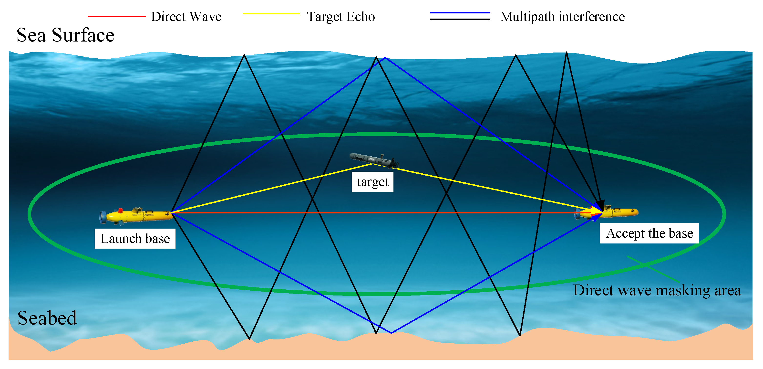
With the continuous advancement in underwater target detection technology, bistatic sonar technology has become a research hotspot in related fields. Compared with monostatic sonar systems, bistatic sonar systems have significant advantages such as strong concealment, high anti-interference ability, and wide detection range [1]. However, when the bi-/multi-static sonar system is in operation, the direct waves from the transmitting base, i.e., the sound waves emitted by the transmitting base and transmitted directly to the receiving base, will interfere with the target echo and even mask it [2]. Especially when the target is in the direct wave-masking area, the direct wave overlaps with the target echo in the time domain, making it difficult to separate them in the time domain [3]. In addition, due to the much shorter propagation path of the direct wave compared to the target echo, its intensity is much greater than that of the echo signal. Moreover, it has a certain correlation with the target echo, which causes serious interference to the detection and positioning of the target [4]. To solve this problem, adaptive filters are widely used in the cancellation process of direct waves due to their excellent performance. When applying adaptive filters for direct wave cancellation, the core task is to accurately estimate the characteristics of the direct wave channel and quickly adapt to the dynamic changes of the channel. This process requires the filter to have a high degree of flexibility and accuracy to ensure effective tracking of changes in direct wave signals and real-time cancellation in the ever-changing underwater environment. Through this method, the impact of direct waves on target echoes can be significantly reduced, thereby improving the system’s ability to detect and locate underwater targets.

Recursive Least Squares (RLS) Adaptive Filter is a widely used algorithm for channel estimation [5]. The traditional RLS algorithm performs effectively in static channels, but its estimation accuracy diminishes in practical scenarios where channels are time varying. For example, in sea or lake environments, surface fluctuations often cause rapid changes in channel conditions [6]. In such dynamic cases, the performance of the classic RLS algorithm in channel estimation significantly decreases. To address this, recent research has focused on improving the adaptability of the RLS algorithm for fast time-varying channels, drawing insights from adaptive filtering and evolutionary approaches in other fields. Techniques such as spectral-kurtosis-based filtering and adaptive mutation strategies, used in fault detection [7] and defect identification [8], respectively, have inspired similar adaptive approaches in RLS algorithms to optimize estimation under complex conditions. These studies support the development of advanced RLS variants with enhanced accuracy and robustness in fluctuating environments.

Zakharov et al. proposed the Divisional Coordinate Descent (DCD) algorithm [9], which reduces the complexity of the algorithm by avoiding complex matrix inversion operations and relying only on addition and shift operations, thereby improving real-time performance. However, although the DCD method significantly improves the efficiency of RLS, simple complexity reduction cannot meet the demand for fast response to channel changes in fast time-varying channel environments. To this end, a sliding window mechanism is introduced, and the SRLS algorithm enhances the tracking ability of time-varying channels by limiting the length of input data [10]. Especially, the SRLS-P algorithm further optimizes its adaptability to time-varying channels by introducing parabolic approximation. However, its computational complexity is still high, and noise accumulation may reduce the estimation accuracy of the algorithm, limiting its performance in high-noise environments. In contrast, Gaussian windows, due to their sidelobe-free spectral characteristics and good smoothness and continuity, can more effectively adapt to the dynamic changes of the channel and reduce sensitivity to abrupt signals. Based on these advantages, this study selects a Gaussian window as the sliding window, aiming to improve the channel estimation performance of the RLS algorithm.

In the paper, we introduce the Variable Gaussian Sliding RLS (VGSRLS) algorithm, based on time-varying Gaussian sliding windows, to address the channel estimation problem posed by the fast time-varying nature of direct wave channels. Traditional fixed-window-length algorithms often struggle to achieve the optimal balance between time and frequency resolution in complex channel environments, leading to decreased estimation accuracy. To tackle this issue, we have designed an adaptive window length adjustment mechanism based on the instantaneous frequency change rate of the signal: when the instantaneous frequency change rate is low, the window length is increased to enhance frequency resolution and processing efficiency; conversely, when the instantaneous frequency change rate is high, the window length is reduced to improve temporal resolution. By dynamically adjusting the Gaussian window length, the algorithm’s accuracy in channel estimation can be significantly improved. To significantly improve the algorithm’s noise suppression capability, we introduce a novel multi-level noise-suppression framework in VGSRLS, which adaptively optimizes the orientation of the Gaussian window using a rotation matrix to ensure alignment with the highest signal-to-noise ratio (SNR) direction within each time frame. Additionally, VGSRLS incorporates an anisotropy factor and a unique dynamic window length adjustment mechanism, which jointly adapt the Gaussian window shape by scaling it along the high-SNR direction. This multi-dimensional adjustment achieves an optimized trade-off between time and frequency resolution, allowing the algorithm to effectively capture rapid variations in non-stationary signals. This multi-dimensional adaptive adjustment strategy, along with the innovative multi-level noise-suppression framework, greatly enhances VGSRLS’s ability to capture fine signal details while achieving substantial improvements in noise resilience, distinguishing it from traditional RLS approaches. To reduce the computational complexity of the VGSRLS algorithm, we employ the DCD algorithm to iteratively solve for the channel estimation values.

2. System Modeling

The system modeling diagram of the bistatic sonar detection system is shown in the following figure. In Figure 1, the transmitted signal x(t) is modulated and amplified by PA. Through the direct wave channel, due to the multipath effect of the channel, signals from multiple paths are superimposed to form a direct wave signal. The hydrophone at the receiving end receives the direct wave signal and ocean noise e(t), forming the received signal y(t) of the bistatic sonar detection system. To ensure effective detection of the echo signal in the future, it is necessary to suppress the direct wave signal. Thus, at the receiving end of the bistatic sonar system, an adaptive filter is used to estimate the direct wave channel and obtain the estimated value of channel $\widehat{h}(i)$.

Assuming there are K multipath paths in the underwater channel, the impulse response function h(t) of the direct wave channel can be modeled as:

$$h(t)={\displaystyle \sum _{k=0}^{K-1}{\alpha }_k}\delta \left(t-{\tau }_k\right)$$

(1)

where ${\alpha }_k$ and ${\tau }_k$ represent the amplitude and delay of the k-th path, respectively.

Through multipath channels, the received signal y(t) can be expressed as:

$$y(t)=x(t)\ast h(t)+e(t)={\displaystyle \sum _{k=0}^{K-1}{\alpha }_k}s\left(t-{\tau }_k\right)+e(t),0\le t\le T_s+{\tau }_{K-1}$$

(2)

where x(t) denotes the transmitted signal, e(t) represents additive noise, $T_s$ represents signal duration, and ${\tau }_{K-1}$ is the maximum latency. We continue to represent the equation in discrete form and define the maximum time delay as:

$$y(t)=x(t)\ast h(t)+e(t)={\displaystyle \sum _{k=0}^{K-1}{\alpha }_k}x\left(t-{\tau }_k\right)+e(t),0\le t\le T_s+{\tau }_{K-1}$$

(3)

3. Time-Varying Gaussian Sliding Window RLS Algorithm

In the system model defined above, the RLS algorithm minimizes the cost function at time n as follows:

$$J_n(h)={\displaystyle \sum _{i=-\infty }^{\infty }w(i-n)}|c(i){|}^2={\displaystyle \sum _{i=-\infty }^{\infty }w(i-n)}|y(i)-x^T(n)h(i){|}^2$$

(4)

where $w(i)$ is the window function and $c(i)$ is the error signal. Due to the multipath effects of underwater acoustic channels and environmental changes such as water flow and temperature gradients, the channel characteristics can rapidly change. The fixed-window-length RLS algorithm has difficulty responding to these changes in a timely manner, which affects the accuracy of channel estimation. To conclude, this article designs a time-varying Gaussian window that automatically adjusts the window length based on the instantaneous frequency change rate of the signal at different time points and combines anisotropy factors to adaptively adjust the shape of the Gaussian window to better adapt to complex channel changes and improve the accuracy of channel estimation.

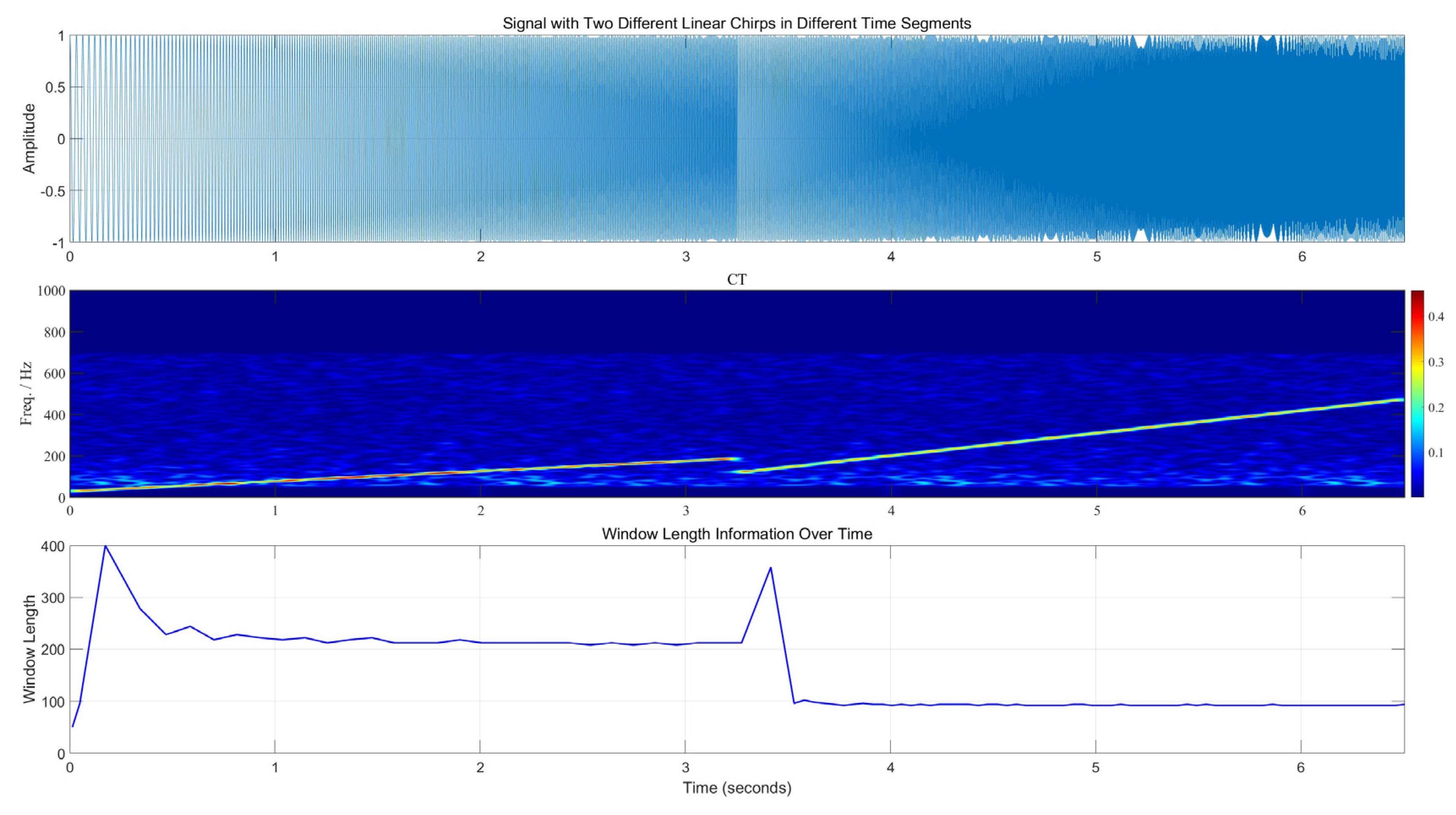
The effectiveness of the Chirplet Transform for non-stationary signals is primarily attributed to its control over the frequency modulation rate. The frequency modulation rate determines how rapidly the Chirplet’s frequency changes, allowing it to flexibly adapt to the time-varying frequency characteristics of the signal. The Chirplet Transform (CT) [11] variation of discrete signals can be expressed as the inner product of signal y(i) and the Chirplet rate, defined as follows:

$$Y(i,f)={\displaystyle \sum _{m=-\infty }^{\infty }y}(m)q_c^{*}(m-i,f)={\displaystyle \sum _{m=-\infty }^{\infty }y}(m)w_{{\sigma }_i}(m-i)e^{j{\displaystyle \frac{a}{2}}{(m-i)}^2}{e}^{-j2\pi fm}$$

(5)

where $i,f,a$ represents the rate of change of signal sample points, signal frequency, and chirplet rate, and $w_{{\sigma }_i}(i)$ is a Gaussian window with a standard deviation of ${\sigma }_i$. In the CT, the chirplet rate parameter controls frequency variation. A higher chirplet rate improves time resolution, enabling CT to capture rapid signal changes. Additionally, $w_{{\sigma }_i}(i)$ in CT adjusts the time spread of the chirplet, where a smaller $w_{{\sigma }_i}(i)$ enhances time resolution but may reduce frequency resolution. Next, we design an optimal $w_{{\sigma }_i}(i)$ using the chirplet rate to balance these resolutions.

CT transformation is linear and singular and can analyze signals through $a$ and rotation angle $\theta$. The rotation angle at each moment is determined by a single $a$,

$$\theta =\arctan \left(2T_s/(F_s\times a)\right)$$

(6)

where $T_s$ and $F_s$ are the sampling time and sampling frequency of the signal, respectively [12].

Use different $a$ values for signals at different time periods. Therefore, the instantaneous linear frequency modulation rate coefficient at the i-th sample point is defined as [13]:

$$\alpha (i,a)=\max \left\{|Y(i,f)|\right\}$$

(7)

when $\alpha (i,a)$ reaches its maximum value, the estimated instantaneous rotation angle of the i-th sample point is:

$$\vartheta (i)=\arg {\max }_c\{\alpha (i,a)\}$$

(8)

Subsequently, calculate the angle value of the instantaneous rotation angle of the i-th sample point based on $\vartheta (i)$, which is $\theta (i)=\arctan \vartheta (i)$. The rate of change $a(i)=\tan (\vartheta (i))\times F_s/(2T_s)$ of the instantaneous frequency of the signal over time. Calculate the CT transform of the signal based on the above content, and then calculate the corresponding $a(i)$ and $\theta (i)$ of the signal at different times according to the different instantaneous linear frequency modulation rates. Next, design Gaussian windows corresponding to different time periods based on $a(i)$ and $\theta (i)$.

For the different instantaneous linear frequency modulation rates of signals in different time periods, the local stationary length at the corresponding time is calculated and defined as follows [14]:

$$M(i)={\max }_{l\ge 0} 2l , {\displaystyle \sum _{m=i-l}^{i+l}|}a(m)-a(m-1)|\le \Delta l$$

(9)

where $M(i)$ is adjusted by the threshold $\Delta l$ and can be obtained by the limit of the frequency modulation rate of the signal. In (8), the length of the Gaussian window is adaptively adjusted based on the instantaneous frequency change rate of the signal. When the instantaneous frequency change rate in the signal is large, a larger time resolution is required, so the window length should be shortened to better track the rapid changes of the signal and suppress the noise components that spread over time. Conversely, when the instantaneous frequency change rate in the signal is small, the length of the window can be appropriately increased to increase the frequency resolution. This helps to distinguish between signals and noise in the frequency domain, increasing the algorithm’s ability to respond quickly to channel changes. By dynamically adjusting the window length, high time resolution or frequency resolution can be maintained at different time periods. This adjustment ensures that the local characteristics of the signal can be effectively adapted when analyzing non-stationary signals. According to the content of reference [15], the standard deviation parameter and width parameter of a Gaussian window can be mutually determined, so the standard deviation of a Gaussian window is:

$$\sigma (i)={\displaystyle \frac{M(i)}{2\sqrt{2\ln 2}}}$$

(10)

In summary, the expression of time-varying Gaussian window [16] in the time domain is:

$$w(i)={\displaystyle \frac{1}{\sqrt{2\pi }\sigma (i)}}{e}^{-{\displaystyle \frac{\kappa appa}{2{\sigma }^2(i)}}}$$

(11)

where,

$$\kappa appa=[i,f]R_{-\theta }[{\lambda }^2,0;0,{\lambda }^{-2}]R_{\theta }{[i,f]}^T$$

(12)

$\theta$ is the direction with the highest signal-to-noise ratio within the window, $R_{\theta }$ is the rotation matrix that rotates the Gaussian window to the direction with the highest signal-to-noise ratio, and the anisotropy factor $\lambda$ is used to control the degree of expansion of the Gaussian window in different directions. Its value can be adaptively adjusted based on the boundary values of the time-frequency characteristics of the signal within the window [17]. The schematic diagram of the formation of a time-varying Gaussian window with known rotation angles $\theta$ and M is shown below.

In Figure 2a, the shape of a regular Gaussian window in the time-frequency plane is influenced by both the window length M and the standard deviation σ. According to the calculation result of Formula (9), the extension of the Gaussian window in the frequency domain can be determined. Therefore, ordinary Gaussian windows exhibit an elliptical shape in the time-frequency plane. In Figure 2b, $R_{-\theta }$ is used to rotate the Gaussian window by θ angle, and the calculation formula is as follows:

$$\left[\begin{array}{c}{i}_2\\ f_2\end{array}\right]=\left[\begin{array}{cc}\cos \theta & -\sin \theta \\ \sin \theta & \cos \theta \end{array}\right]\left[\begin{array}{c}{i}_1\\ f_1\end{array}\right]$$

(13)

where ${\left[\begin{array}{cc}{i}_1& f_1\end{array}\right]}^{\mathrm{T}}$ is the original coordinate of the Gaussian window, and ${\left[\begin{array}{cc}{i}_2& f_2\end{array}\right]}^{\mathrm{T}}$ is the coordinate of the Gaussian window after being rotated by a rotation matrix by θ angle. This step changes the direction of the Gaussian window to point towards the direction with the highest signal-to-noise ratio. In Figure 2c, the time resolution and frequency resolution of the rotated Gaussian window are controlled by stretching and compressing it using $[{\lambda }^2,0;0,{\lambda }^{-2}]$. The Gaussian window is stretched to ${\lambda }^2\ast M$ in the time domain and compressed to $M_1/{\lambda }^2$ in the frequency domain, thereby improving frequency resolution. Compared to the case of using a regular Gaussian window in Figure 2a, the rotated and scaled Gaussian window has a significant suppression effect on the noise inside the window, thereby improving the signal-to-noise ratio of the signal inside the window. In Figure 2d, the time-varying Gaussian window is rotated back to its original coordinate system using $R_{\theta }$, and the calculation formula is as follows:

$$\left[\begin{array}{c}{i}_3\\ f_3\end{array}\right]=\left[\begin{array}{cc}\cos \theta & \sin \theta \\ -\sin \theta & \cos \theta \end{array}\right]\left[\begin{array}{c}{i}_2\\ f_2\end{array}\right]$$

(14)

where ${\left[\begin{array}{cc}{i}_3& f_3\end{array}\right]}^{\mathrm{T}}$ and ${\left[\begin{array}{cc}{i}_1& f_1\end{array}\right]}^{\mathrm{T}}$ are in the same coordinate system, in order to distinguish the values of the Gaussian window before rotation and after inverse rotation. Reverse rotation ensures that the Gaussian window and signal are analyzed in the same coordinate system, maintaining the unity of time-frequency analysis and facilitating subsequent signal processing and applications. When λ = 1, the anisotropic Gaussian window degenerates into an isotropic Gaussian window.

In time-varying Gaussian windows, the main function is to improve temporal resolution by adjusting the length of the Gaussian window; by adjusting the anisotropy factor, it mainly works to improve frequency resolution. Therefore, these two processes are complementary: (1) when the signal frequency changes rapidly, the window length is shortened to maintain a high time resolution; (2) by adjusting the shape of the Gaussian window, the optimal resolution can be maintained on the frequency axis. In a time-varying Gaussian window, the adjustment of window length M and the adjustment of shape are coordinated with each other. By dynamically adjusting the window length to optimize time resolution and adjusting the window shape to enhance frequency resolution, optimal results can be achieved in complex non-stationary signal analysis. The adaptive Gaussian window in this framework is specifically designed to enhance noise suppression in real-world, non-stationary environments by dynamically adjusting its shape and orientation. This adaptability allows the algorithm to better isolate desired signals from background noise, significantly improving the signal-to-noise ratio within the analysis window.

According to the Gaussian window w with adaptive adjustment of window length designed above, the solution caused by minimizing the cost function of the signal in the window according to (4) is:

$$\hat{\mathrm{h}}(i)={\mathbf{S}}^{-1}(i)\beta (i)$$

(15)

where $\mathbf{S}(i)$ is the autocorrelation matrix of $L\times L$, $\beta (i)$ is the cross-correlation vector of $L\times 1$, and their definitions are:

$$\mathbf{S}(i)={\displaystyle \sum _{j\in \Gamma }w}(j)\mathbf{x}(i+j){\mathbf{x}}^H(i+j)$$

(16)

$$\mathbf{\beta }(i)={\displaystyle \sum _{j\in \Gamma }w}(j)\mathbf{x}(i+j){\mathbf{y}}^{*}(i+j)$$

(17)

where $\Gamma$ is the range of the time-varying Gaussian window at this moment. For each moment i, in order to calculate the channel estimate, it is necessary to compute the inverse of the autocorrelation matrix $\mathbf{S}(i)$. This is the most complex step of the RLS algorithm and also the reason for its high computational complexity. A new method for calculating autocorrelation matrix was proposed in reference [18],

$${[\mathbf{S}(i)]}_{m+1,n+1}={[\mathbf{S}(i-1)]}_{m,n}$$

(18)

where ${\mathbf{S}}_{m,n}$ represents the m-th column and n-th row of matrix s. Therefore, only the information in the first column of matrix $\mathbf{S}(i)$ needs to be calculated to update matrix $\mathbf{S}(i)$. The formula for calculating ${\mathbf{S}}^{(1)}(i)$ is:

$${\mathbf{S}}^{(1)}(i)={\displaystyle \sum _{j\in \Gamma }w}(j)\mathrm{x}(i+j){\mathbf{x}}^{*}(i+j)={\displaystyle \sum _{j\in \Gamma }\tilde{w}}(i,j){\mathbf{x}}^{*}(i+j)$$

(19)

where $\tilde{w}(i,j)=w(j)x(i+j),j\in \Gamma ,$ the data length is consistent with the length M of the Gaussian window. ${\mathbf{S}}^{(1)}(i)$ can be considered as the convolution of $\tilde{w}(i,j)$ vector and ${\mathbf{x}}^{*}(i+j)$ vector. Therefore, to improve the computational speed of the algorithm, the time-domain convolution operation is converted into a frequency-domain multiplication operation.

$${\mathbf{S}}^{(1)}(i)=\mathrm{IFFT}(D_w\odot D_x)$$

(20)

where,

$$D_w=\mathrm{FFT}(\tilde{w}(i))$$

(21)

$$D_x=\mathrm{FFT}({\mathbf{x}}^{*}(i))$$

(22)

Since the $\mathbf{S}(i)$ matrix is an Hermitian matrix, the elements in the first row of $\mathbf{S}(i)$ are equal to the elements in the first column of $\mathbf{S}(i)$. Thus, the update of the $\mathbf{S}(i)$ matrix is completed.

After calculating the $\mathbf{S}(i)$ matrix, the main complexity of the algorithm lies in the inverse of the $\mathbf{S}(i)$ matrix. In order to reduce the complexity of the algorithm and improve its stability, matrix inversion should be avoided. Therefore, in order to accurately estimate the channel estimation $\widehat{\mathbf{h}}(i)$, the following equation is solved:

$$\beta (i)=\mathbf{S}(i)\widehat{\mathbf{h}}(i)$$

(23)

Iteratively solve the above equation to obtain an approximate value of the channel impulse response. In order to further reduce the complexity of the algorithm, this paper uses Dichotomous Coordinated Descent (DCD) to iteratively solve the above equation. In each iteration, the DCD algorithm updates the component in vector $\widehat{\mathbf{h}}(i)$ that corresponds to the element with the highest amplitude in $\beta (i)$. The algorithm updates from four directions [−1, 1, −j, j] and selects the direction that minimizes the cost function to complete a successful iteration. If the updates in all four directions cannot reduce the cost function, then the step size H is halved and the above process is repeated until the step size is reduced to the minimum value or the maximum number of iterations is reached. The maximum number of times the step size is reduced, $M_b$, corresponds to the number of bits required for the solution vector. Due to the fact that the DCD algorithm does not require multiplication or division operations, its complexity depends on the number of successful iterations $N_u$. Therefore, when dealing with different time-varying systems, an appropriate $N_u$ should be selected.

For each iteration, the complexity of the VGSRLS algorithm can be approximated as $O(N{M}_{avg})$, where N is the data length and $M_{avg}$ represents the average window length.

Given that the VGSRLS algorithm incorporates a dynamic window-length adjustment mechanism, we use the average window length $M_{avg}$ in the complexity analysis to better reflect the overall complexity of the algorithm. According to [12], The MACs of CT are $5M_{\mathrm{avg}}{N}_1\log N_1$, where $N_1$ is the number of chirplets, and $M_{avg}$ represents the average window length. The VGSRLS algorithm also employs the Leading DCD iterative algorithm for solving the problem. According to [9], the MACs for the Leading DCD algorithm are $2(M_{\mathrm{avg}}+1)N_u+M_b$. Therefore, the total MACs for the VGSRLS algorithm are $2(M_{\mathrm{avg}}+1)N_u+M_b+5M_{\mathrm{avg}}{N}_1\log N_1$.

The pseudocode of the VGSRLS algorithm is shown in Algorithm 1, and the pseudocode of the time-varying Gaussian window is shown in Algorithm 2.

Algorithm 1. VGSRLS Algorithm.
Step	Input: x(i), y(i), N, $N_u$, $M_b$ and H
	Output: $\widehat{\mathbf{h}}(i)$
	Initialization: $\widehat{\mathbf{h}}(i)=0,\mathrm{S}(i)=0$
1	CT:$Y(i,f)={\displaystyle \sum _{m=-\infty }^{\infty }y}(m)w_{{\sigma }_i}(m-i)e^{j{\displaystyle \frac{a}{2}}{(m-i)}^2}{e}^{-j2\pi fm}$
2	for i = 1,2, …., N
3	Calculate the Gaussian window at the current time $w(i)$
4	$D_w=\mathrm{FFT}(\tilde{w}(i)),D_x=\mathrm{FFT}({\mathbf{x}}^{*}(i)).{\mathbf{S}}^{(1)}(i)=IFFT(D_w\odot D_x)$
5	$c^{*}(i)=y(i)-{\hat{\mathrm{h}}}^H(i-1)\mathrm{x}(i-1), \mathrm{y}(i)=\mathrm{w}(i)c^{*}(i),$ $D_y=\mathrm{FFT}( \mathrm{y}(i\left)\right),r(i)=\mathrm{IFFT}(D_x\odot D_y)$
6	Using DCD to solve Equation (23)
7	$\widehat{\mathbf{h}}(i)=\widehat{\mathbf{h}}(i-1)+\Delta \mathbf{h}(i)$

Algorithm 2. Calculation of time-varying Gaussian window.
Step	Input: $Y[i,f]$
	Output: M and $\sigma$
	Initialization: $\alpha (i)=0,a=0,\vartheta (i)=0$
1	$\alpha (i,a)=\max \left\{|Y(i,f)|\right\}$
2	$\vartheta (i)=\arg {\max }_c\{\alpha (i,a)\},\theta (i)=\arctan \vartheta (i)$
3	$a(i)=\tan (\vartheta (i))\times F_s/(2T_s)$
4	$M[i]={\max }_{l\ge 0} 2l, {\displaystyle \sum _{m=i-l}^{i+l}|}a[m]-a[m-1]|\le \Delta l$
5	Calculate $\sigma (i)$ using Equation (10)

When the channel is a constant channel, the transmission characteristics of the signal remain constant over time and will not change due to differences in time. This characteristic means that the impulse response or frequency response of the channel is the same at any point in time. In this case, the instantaneous frequency change rate of the signal depends on the characteristics of the signal itself, and its value is constant. At this point, Equation (8) becomes:

$$M[i]={\max }_{l\ge 0} 2l, 2l*a_1\le \Delta l$$

(24)

The window length of the Gaussian window is no longer adjusted according to the frequency change rate and becomes a fixed value. The adaptive adjustment of the Gaussian window shape is mainly based on the spectral characteristics of the signal and the directionality of the signal-to-noise ratio. In a time-invariant channel, the spectral characteristics of the signal are stable and the directionality is fixed, while the Gaussian window degenerates into a shape and direction fixed on the time-frequency plane. The expression of the Gaussian window function after degradation is:

$$w(i)={\displaystyle \frac{1}{\sqrt{2\pi }\sigma }}{e}^{-{\displaystyle \frac{i^2}{2{\sigma }^2}}}$$

(25)

4. Simulation

4.1. Introduction to Simulation Experiment

We have built a simulation platform for a bistatic sonar detection system using Matlab 2023b, as shown in Figure 3. In a bistatic sonar detection system, there are not only target echoes, but also direct wave interference from the transmitting end to the receiving end. Therefore, in order to accurately detect the target echo, it is necessary to cancel the direct wave signal, and accurate estimation of the direct wave channel is crucial in this process.

Simulate the direct wave channel through Bellhop according to the above schematic diagram. In the simulation environment, the depth of the transmitting end of the bistatic sonar detection system is 10 m, the horizontal distance from the receiving end is 1 km, and the depth of the receiving end is 20 m. Simulate the propagation path of direct wave signals in the above simulation environment, according to the shallow water sound velocity data obtained from testing at the National Marine Test Site. Afterwards, the transmitting end was set in the simulation software as shown in Figure 4 to simulate the direct wave channel, and the simulation results are shown in Figure 5.

In Figure 5, the red circle represents the transmitting end of the bistatic sonar detection system, and the red rectangle represents the receiving end of the bistatic sonar detection system. There are intrinsic sound rays between the transmitting and receiving ends, which only undergo one reflection from the seabed or sea surface to reach the receiving end. The color of the intrinsic sound rays is blue. The intrinsic sound rays that have been reflected multiple times from the seabed surface and reached the receiving end are black in color. From the figure, it can be observed that there are multiple taps in the direct wave channel. If channel estimation is not performed on them, it will affect the subsequent target echo detection. In the following simulation experiments, the VGSRLS algorithm is used to estimate the direct wave channel and verify the channel estimation performance of the VGSRLS algorithm.

To verify that the VGSRLS algorithm can adapt to the instantaneous frequency change rate of signals and enhance its ability to track channel changes, consider a composite signal consisting of two LFM signals with a length of 1 s, where the LFM starting frequencies from 0 to 3.25 s and from 3.25 s to 6.5 s are 20 Hz and 200 Hz, respectively, and the ending frequencies are 120 Hz and 500 Hz, respectively. As shown in Figure 6, after the initialization phase, VGSRLS adaptively adjusts the window length to around 212 during the first LFM signal phase; when entering the second stage of LFM signal, as the signal change rate increases, the VGSRLS algorithm adaptively shortens the window length to around 94, thereby enhancing the time resolution and improving the accuracy of the algorithm in estimating the channel.

4.2. Simulation Experiment and Result Analysis

To verify the superiority of the VGSRLS algorithm, we conducted numerical simulation experiments following the methodologies outlined in the literature [18,19]. We compare it with the SRLS-DCD algorithm. Furthermore, to compare it with the latest adaptive algorithms, we also evaluated it against the finite-window Recursive Least Squares (FRLS) algorithm proposed in reference [20]. According to the system modeling in Formula (3), $\mathbf{x}(i)$ is the input signal, whose elements are zero mean, uncorrelated complex Gaussian numbers with a variance of 1. $\mathbf{h}(i)$ is the impulse response of the system to be identified. This study adopts the ocean noise model presented in reference [21], which is valid across the frequency spectrum from 10 Hz to 100 kHz. Using environmental data collected from the mid-Atlantic, as detailed in the aforementioned study, the power spectral density of ocean noise was computed and used as the noise model for this research. The time-varying channel in the system to be identified consists of 50 taps, each modeled as an independent zero-mean, unit-variance random process with uniform power spectral density within the frequency range $[-f_{max},f_{max}]$ [10]. To ensure the randomness of the tap, the Fast Fourier Transform (FFT) method was used for generation [22]. To accurately simulate underwater channel variations, a frequency interval of $[-f_{max},f_{max}]$ is used, with $f_{max}$ between 0.1 Hz and 1 Hz, each corresponding to distinct sea conditions. At 1 Hz, the model reflects short-period wind waves typically associated with strong local winds and moderate to high sea states, where waves are steep with shorter wavelengths. In contrast, 0.1 Hz represents long-period swells from distant storms, with smoother, longer-wavelength waves [23].

To quantify the performance of the proposed algorithm, we chose mean squared deviation (MSD) as the evaluation metric for the experiment. The smaller the MSD value, the more accurate the algorithm is in estimating the underwater channel. To avoid randomness, we conducted a total of 60 simulation experiments, and the average value of the experiments was taken as the experimental result of the algorithm. The MSD for each simulation experiment is:

$$\mathrm{MSD}(i)=\Vert \mathbf{h}(i)-\widehat{\mathbf{h}}(i){\Vert }_2^2/E_h$$

(26)

where $\widehat{\mathbf{h}}(i)$ is the channel estimation value, $E_h=(1/N){\displaystyle \sum _{i=1}^N|}|\mathbf{h}(i)|{|}^2$, and N is the number of samples after the algorithm converges. The above formula calculates the average value of MSD on these N samples after the algorithm converges. In the simulation experiment, for fast time-varying systems, $f_{\max }$ is set to 1 Hz. The simulation results of the channel estimation performance of various algorithms for fast time-varying systems when the SNR changes from −5 dB to 10 dB are shown in the following figure.

From the simulation results in Figure 7, it can be seen that as the SNR increases, the MSD performance of all algorithms improves. This indicates that at lower noise levels, the algorithm can estimate the channel more accurately, thereby reducing errors. Overall, the VGSRLS algorithm exhibits lower MSD values at various signal-to-noise ratio levels, demonstrating its superiority in signal estimation. The SRLS-DCD (M = 100) algorithm performs well in the low-to-medium signal-to-noise ratio range, but as the signal-to-noise ratio further improves, its performance improvement rate slows down, showing a certain performance bottleneck. When M = 200, the MSD performance of the algorithm immediately improves to a certain extent. The FRLS algorithm also exhibits similar performance; although its estimated channel performance is better than SRLS, it still lags behind VGSRLS algorithm in high noise environments. This indicates that in fast time-varying channels, a fixed window length cannot flexibly adapt to the rapid changes in the channel, which will limit the MSD performance of the algorithm. The excellent performance of the VGSRLS algorithm is mainly attributed to its dynamic window length adjustment strategy and adaptive adjustment of window shape. Faced with rapidly changing channels, the VGSRLS algorithm can automatically adjust the width of its Gaussian window to cope with sharp changes in signal frequency, thereby improving time resolution and optimizing the MSD performance of the algorithm. Under high-noise environmental conditions, the VGSRLS algorithm uses a rotation matrix to adaptively adjust the direction of the Gaussian window, ensuring that the window is always aligned with the direction with the highest signal-to-noise ratio. In addition, the algorithm combines dynamic adjustment of window length and anisotropy factor, adaptively adjusting the window shape along the direction with the highest signal-to-noise ratio, effectively suppressing noise interference in other directions. These mechanisms work together to significantly improve the overall performance of the algorithm, enabling it to exhibit outstanding performance in low signal-to-noise ratio and fast time-varying systems.

Next, SNR = 5 dB, and the channel variation parameter $f_{\max }$ changes from 0.1 Hz to 1 Hz. The simulation results are shown in Figure 8. From the graph, it can be observed that as the speed of channel changes increases, the MSD performance of all algorithms decreases. This is because the rapid changes in the channel increase the difficulty of channel estimation, but the MSD performance of the VGSRLS algorithm still remains optimal. Under the condition of a window length of 100, the SRLS-DCD algorithm performs well at low channel change rates, but its MSD performance deteriorates rapidly with increasing $f_{\max }$, indicating insufficient adaptability to channel changes. When M = 200, the MSD performance of the SRLS-DCD algorithm is lower when $f_{\max }$ is low, but as $f_{\max }$ increases, the MSD performance of the algorithm gradually deteriorates. As the rate of channel changes becomes faster, the performance of the FRLS algorithm in estimating the channel also shows a certain decline. The VGSRLS algorithm can maintain superior MSD performance and relatively stable MSD performance even at low SNR as the channel change rate increases. This is because the VGSRLS algorithm ensures that the Gaussian window is stretched and compressed along the direction with the highest signal-to-noise ratio during scale transformation based on the rotation matrix, effectively reducing the interference of noise in other directions. When scaling the Gaussian window again, it can effectively balance the time resolution and frequency resolution of the algorithm, further enhancing its anti-noise performance.

5. Conclusions

This article presents the VGSRLS adaptive filtering algorithm, which incorporates a dynamic sliding-window adjustment mechanism, dual rotation matrices, and an anisotropy factor to adaptively adjust the Gaussian window shape, significantly enhancing the estimation performance of the RLS algorithm in underwater acoustic channels. By adaptively tuning the Gaussian window shape on the time-frequency plane through dynamic window length adjustments and anisotropy factors, the VGSRLS algorithm can effectively track rapidly fluctuating frequency channels, achieving high resolution and stable channel estimation performance in complex, fast-changing environments. The inclusion of the rotation matrix further bolsters the algorithm’s noise resistance, aligning the Gaussian window with the direction of the highest signal-to-noise ratio to minimize interference from noise in other directions. Through this multi-level adaptive design, the VGSRLS algorithm demonstrates strong performance in estimating direct wave channels in challenging underwater acoustic communication environments. The VGSRLS algorithm’s reduced computational overhead, achieved through DCD iterative solving and efficient FFT transformation, enhances its feasibility for real-time applications in dynamic underwater acoustic communication systems. This makes it suitable for scenarios where low-latency and high-efficiency channel estimation are crucial. Simulation experiments confirm that the VGSRLS algorithm outperforms both the SRLS-DCD and FRLS algorithms under typical underwater ambient noise levels and channel variations, which emphasizes its effectiveness. In our future research, we will focus on conducting a deeper theoretical analysis of the convergence properties and stability of the VGSRLS algorithm under typical underwater conditions. Additionally, we plan to implement the VGSRLS algorithm on Field-Programmable Gate Arrays (FPGAs) for real-world underwater experiments to validate its effectiveness in practical underwater environments.

References

1. Zhao, B.; Che, Y. Overview of the Bistatic/Muriatic Sonar Technology. In Proceedings of the 2009 National Academic Exchange Conference on Hydroacoustics and the Election of the Hydroacoustics Branch, Dalian, China, 19–23 June 2009; Naval Submarine Academy: Qingdao, China, 2009. [Google Scholar]
2. Zhou, Z. Target Detection and Direct Wave Suppression of Multistatic Sonar System. Master’s Thesis, Harbin Engineering University, Harbin, China, 2022. [Google Scholar]
3. Liang, G.; Zhou, Y.; Qiu, L. Real time calibration method for flexible horizontal waveform detection using dual base active detection. J. Acoust. 2023, 48, 831–842. [Google Scholar]
4. Wang, Y. Research on Algorithm for Strong Interference Suppression of Bistatic Sonar. Master’s Thesis, Harbin Engineering University, Harbin, China, 2023. [Google Scholar]
5. Wei, M. Research and Implementation of the Key Technology of Multiple Diversity Reception for HF Communication. Master’s Thesis, Xi’an University of Electronic Science and Technology, Xi’an, China, 2012. [Google Scholar]
6. Jiang, W.; Tong, F.; Zhu, Z. Exploiting Rapidly Time-Varying Sparsity for Underwater Acoustic Communication. IEEE Trans. Veh. Technol. 2022, 71, 9721–9734. [Google Scholar] [CrossRef]
7. Vashishtha, G.; Chauhan, S.; Zimroz, R.; Kumar, R.; Gupta, M.K. Optimization of spectral kurtosis-based filtering through flow direction algorithm for early fault detection. Measurement 2025, 241, 115737. [Google Scholar] [CrossRef]
8. Chauhan, S.; Singh, M.; Aggarwal, A.K. Bearing defect identification via evolutionary algorithm with adaptive wavelet mutation strategy. Measurement 2021, 179, 109445. [Google Scholar] [CrossRef]
9. Zakharov, Y.V.; White, G.P.; Liu, J. Low-complexity RLS algorithms using dichotomous coordinate descent iterations. IEEE Trans. Signal Process. 2008, 56, 3150–3161. [Google Scholar] [CrossRef]
10. Shen, L.; Zakharov, Y.; Henson, B.; Morozs, N.; Mitchell, P.D. Adaptive Filtering for Full-Duplex UWA Systems with Time-Varying Self-Interference Channel. IEEE Access 2020, 8, 187590–187604. [Google Scholar] [CrossRef]
11. Hildebrand, J.A. Anthropogenic and natural sources of ambient noise in the ocean. Mar. Ecol. Prog. Ser. 2009, 395, 5–20. [Google Scholar] [CrossRef]
12. Mann, S.; Haykin, S. Adaptive “chirplet” transform: An adaptive generalization of the wavelet transform. Opt. Eng. 1992, 31, 1243–1256. [Google Scholar] [CrossRef]
13. Yu, G.; Zhou, Y. General linear chirplet transform. Mech. Syst. Signal Process. 2016, 70–71, 958–973. [Google Scholar] [CrossRef]
14. Miao, Y.; Li, J.; Sun, H. Multimodal Sparse Time-Frequency Representation for Underwater Acoustic Signals. IEEE J. Ocean. Eng. 2021, 46, 642–653. [Google Scholar] [CrossRef]
15. Chen, Y. Research on Key Technologies of F-OFDM for 5G. Master’s Thesis, University of Electronic Science and Technology, Chengdu, China, 2020. [Google Scholar]
16. Miao, Y. Research on Recognition Technologies for Underwater Acoustic Signals from Multiple Targets. Master’s Thesis, Xiamen University, Xiamen, China, 2021. [Google Scholar]
17. Shen, L.; Zakharov, Y.; Shi, L.; Henson, B. BEM Adaptive filtering for SI cancellation in full-duplex underwater acoustic systems. Signal Process. 2022, 191, 108366. [Google Scholar] [CrossRef]
18. Carmona, R.A.; Hwang, W.L.; Torresani, B. Multiridge detection and time-frequency reconstruction. IEEE Trans. Signal Process. 1999, 47, 480–492. [Google Scholar] [CrossRef]
19. Oberlin, T.; Meignen, S.; Perrier, V. Second-order synchrosqueezing transform or invertible reassignment? Towards ideal time-frequency representations. IEEE Trans. Signal Process. 2015, 63, 1335–1344. [Google Scholar] [CrossRef]
20. Shen, L.; Zakharov, Y.; Niedźwiecki, M.; Gańcza, A. Finite-window RLS algorithms. Signal Process. 2022, 198, 108599. [Google Scholar] [CrossRef]
21. Tollefsen, C.D.; Pecknold, S. A Simple Yet Practical Ambient Noise Model; Defence Research and Development Canada: Ottawa, ON, Canada, 2022. [Google Scholar]
22. Percival, D.B. Simulating Gaussian random processes with specified spectra. Comput. Sci. Stat. 1993, 24, 534–538. [Google Scholar]
23. Sayed, A.H. Fundamentals of Adaptive Filtering; John Wiley & Sons: Hoboken, NJ, USA, 2003. [Google Scholar]
Figure 1. Modeling diagram of bistatic sonar detection system.
Jmse 12 02185 g001
Figure 2. Schematic diagram of time-varying Gaussian window. (a) Determine the Gaussian window with window length M. (b) Rotate the Gaussian window according to θ. (c) Scaling the rotated Gaussian window. (d) Rotate the Gaussian window back to the original coordinate system.
Jmse 12 02185 g002
Figure 3. Schematic diagram of simulation platform.
Jmse 12 02185 g003
Figure 4. Sound Velocity Profile of National Marine Test Site.
Jmse 12 02185 g004
Figure 5. Simulation diagram of direct wave channel.
Jmse 12 02185 g005
Figure 6. TVGSRLS variable window length performance verification.
Jmse 12 02185 g006
Figure 7. Comparison of MSD performance of various algorithms in identifying fast time-varying systems.
Jmse 12 02185 g007
Figure 8. Comparison of MSD performance of various algorithms in identifying time-varying systems at different channel variation rates under SNR= 5 dB.
Jmse 12 02185 g008
Disclaimer/Publisher’s Note: The statements, opinions and data contained in all publications are solely those of the individual author(s) and contributor(s) and not of MDPI and/or the editor(s). MDPI and/or the editor(s) disclaim responsibility for any injury to people or property resulting from any ideas, methods, instructions or products referred to in the content.