Article

Simulation Method and Application of Non-Stationary Random Fields for Deeply Dependent Seabed Soil Parameters

1
Institute of Geotechnical Engineering, Nanjing Tech University, Nanjing 211816, China
2
School of Geology and Mining Engineering, Xinjiang University, Urumqi 830049, China
*
Authors to whom correspondence should be addressed.
J. Mar. Sci. Eng. 2024, 12(12), 2183; https://doi.org/10.3390/jmse12122183
Submission received: 31 October 2024 / Revised: 25 November 2024 / Accepted: 27 November 2024 / Published: 28 November 2024
(This article belongs to the Section Coastal Engineering)

Abstract

:
The spatial variability of geotechnical parameters, such as soil shear wave velocity (Vs), exhibits significant nonlinearity and non-stationarity with respect to depth (h) due to the influence of overlying stress. Existing stochastic field models for describing the variability of geotechnical parameters are insufficient for simultaneously capturing both the nonlinearity and non-stationarity of these parameters. In this study, a power function Vs = Vs0[f(h)]n is proposed to describe the nonlinear trend in soil shear wave velocity (Vs) as a function of depth-related variable f(h). Considering the physical significance and correlation of the power function parameters Vs0 and n, the variability of these parameters is modeled using a random variable model and a stationary stochastic field model, respectively. This leads to the development of a non-stationary stochastic field model that describes the spatial variability of Vs. The proposed method is applied to simulate the random Vs-structure of a seabed site in China, and the obtained Vs results are used to assess the liquefaction probability of the seabed. The results indicate that ignoring the correlation between geotechnical parameters significantly increases the variability of the final simulation results. However, the proposed method accurately captures the nonlinear trend and non-stationary characteristics of soil Vs with depth, and the liquefaction probability predictions are consistent with those derived from in situ Vs measurements in the study area. This approach provides valuable guidance for simulating the spatial variability of depth-dependent geotechnical parameters, particularly those significantly influenced by overlying pressure.

1. Introduction

1.1. Soil Liquefaction Risk and Impact

Under the influence of cyclic loads generated by earthquakes, the effective stress experienced by the soil skeleton in saturated sands gradually transitions to pore water pressure. This shift results in a loss of strength and stiffness within the soil mass, ultimately leading to its liquefaction. Soil liquefaction can cause various detrimental effects, including ground settlement, building tilting, buoyancy of underground pipelines, lateral displacement of riverbanks, bridge collapse, dam sliding, and damage to underground structures and dock facilities. Over the past two decades, large-scale liquefaction events and the significant destruction of surface structures and underground facilities they cause have repeatedly occurred during catastrophic earthquakes worldwide. Consequently, conducting site-specific earthquake liquefaction risk assessments has become an urgent priority in geotechnical engineering [1].
Soil liquefaction triggered by earthquakes is a potential risk that must be considered in marine engineering. The 1999 Izmit earthquake in Turkey (Moment magnitude Mw = 7.4), the 2011 Christchurch earthquake in New Zealand (Mw = 6.2), and the 2011 Great East Japan earthquake (Mw = 9.0) demonstrated that newly deposited alluvial soils near coastlines and artificially filled soils, particularly those containing fine particles and gravel with short consolidation periods, are prone to severe liquefaction. These events caused rare and extensive liquefaction in the Izmit Bay area, central Christchurch, and Tokyo Bay [2,3,4]. Additionally, other natural disasters can indirectly trigger soil liquefaction. For example, heavy rainfall, debris flows caused by volcanic eruptions, or landslides can raise groundwater levels, alter water flow paths, or change the moisture content of soil layers, potentially leading to structural changes in the soil. The risk of localized liquefaction increases, especially when these disasters expose previously compacted soil layers.

1.2. Spatial Variability of Geotechnical Parameters

Currently, the most widely used method for evaluating the potential for earthquake-induced liquefaction at a site is the semi-empirical approach based on the standard penetration test (SPT) and the peak ground acceleration (amax) caused by earthquakes [2,3,4,5,6,7]. However, the SPT can significantly disturb soil layers, and the test data often exhibit considerable variability [8,9,10,11]. The shear wave velocity (Vs) testing method is an alternative in situ testing approach that effectively addresses the shortcomings of the SPT. For example, the SPT is not sensitive to variations between soil layers and fails to accurately reflect the impact of significant layer changes. Additionally, the stability of the hammer energy is poor, and the test is less effective for larger grain-sized samples. Furthermore, due to the limited test depth, it cannot effectively assess the properties of deeper soils. These factors represent the limitations of the SPT. Furthermore, Vs is a physical quantity directly related to the small-strain shear modulus, which reflects the fundamental mechanical properties of the soil [12]. Consequently, the site liquefaction assessment method based on shear wave velocity and peak ground acceleration has promising applications. Site-specific shear wave velocity prediction models are typically developed using deterministic methods, which can be divided into two types. The first type uses borehole data and interpolation techniques to create a deterministic Vs distribution at locations without boreholes. However, this approach does not account for the various possible Vs distributions between boreholes [13,14]. The second method uses regression analysis to establish a relationship between shear wave velocity and depth (h). This approach is limited to one-dimensional site models and does not capture the variability of shear wave velocity in different two-dimensional spatial orientations [15].
Geotechnical parameters show significant spatial variability due to complex deposition conditions and human engineering activities [16,17,18,19,20]. For example, shear wave velocity is often measured during field exploration, but this parameter is influenced by factors like stratum type, depth, and deposition environment [21,22]. Even within the same site, shear wave velocity can vary significantly, especially at stratum boundaries [23]. Additionally, geotechnical parameters at different locations may exhibit correlations [24,25]. Stochastic field models are useful for representing the spatial variability and correlations of geotechnical parameters [24,26,27,28,29,30,31,32]. To improve computational efficiency, stationary stochastic field models with fixed means and standard deviations are commonly used [28,33,34,35,36]. Research indicates that the mean and standard deviation of geotechnical parameters, such as undrained shear strength, SPT blow counts, and shear wave velocity, vary with depth and are influenced by overburden pressure [16,19,20,37,38]. Griffiths and Fenton applied non-stationary stochastic fields to model shear strength variability with depth in slope soils, improving slope stability analysis [28]. Shuihua Jiang and Jinsong Huang divided soil parameter variability into trend and random fluctuation components to describe non-stationary stochastic fields, focusing on undrained shear strength variability [39].

1.3. Depth-Dependent Non-Stationary Stochastic Field

In the aforementioned research on non-stationary stochastic fields, the trend function that describes the variation of geotechnical parameter means with depth is typically linear [40,41,42,43]. However, the corresponding methods often overlook the interdependence among the parameters within the trend function when determining the variation of geotechnical parameter means and standard deviations with h [17,18]. For soil parameters that are significantly influenced by overburden pressure, the statistical characteristics often exhibit nonlinear trends along the burial depth [39,44,45,46].
When employing complex nonlinear models to describe the variation of geotechnical parameters with depth, it can be challenging to directly derive the variability of these parameters through analytical methods. In such instances, the variability of the parameters within the nonlinear model, combined with error propagation theory, can be utilized to approximate the variability of geotechnical parameters with depth. The point estimate method is a straightforward and effective approach for analyzing error propagation. This method leverages the variability of parameters in simulations to estimate the uncertainty of model predictions through simple algebraic operations while also accounting for the correlations between model parameters [45,47].

1.4. Site Characterization and Methodology

Taking a site in Hai’an City, Jiangsu Province, as an example, random Vs-structure simulation is conducted for the target site based on existing boreholes ZK1–ZK30, and the liquefaction risk at the site is evaluated. The study area is located in the lower reaches of the Yangtze River to the South Yellow Sea seismic belt, which belongs to the North China seismic zone, an area with moderate to high frequency of seismic activity. The focal depths are mainly concentrated between 10 and 20 km. In particular, the site exhibits a typical Vs-structure with multiple sedimentary layers. The surface layer is predominantly composed of soft to medium soils (with Vs values around 80–300 m/s), while deeper layers consist of dense to very dense soils. Notably, the shear wave velocity shows a nonlinear increase with depth, reflecting the transition from loose to more consolidated materials. These characteristics make the site a representative example of the region’s seismic response behavior, particularly in relation to the depth-dependent Vs profile.
Furthermore, the paper applies measured borehole data from Hai’an City and uses a nonlinear power function to model the relationship between shear wave velocity (Vs) and depth (h). The method is suited for evaluating seismic-induced soil liquefaction, as it captures the variability and intercorrelation of soil parameters, crucial for accurate liquefaction assessments. To account for parameter intercorrelation, the point estimate method is used to quantify the mean and standard deviation of Vs with depth. Statistical information from the fitting parameters is then employed to generate a stationary stochastic field, considering parameter intercorrelation, through the Kaiser–Dickman sampling algorithm. These simulated parameters are substituted into the power function, creating a non-stationary stochastic field that reflects the spatial variability of Vs. This approach overcomes the limitations of previous studies that rely on linear functions, which ignore parameter intercorrelation. The results are particularly applicable to the specific seabed stratigraphy in the study area, where the method provides a more accurate representation of soil heterogeneity. By integrating the stochastic Vs distribution with a liquefaction model, the soil’s liquefaction potential is assessed, and the liquefaction probability distribution is determined. This analysis emphasizes the impact of parameter intercorrelation and spatial autocorrelation on the variability of Vs and liquefaction evaluation.

2. Stochastic Simulation Method for Vs-Structure

The integration of actual borehole data with geological modeling techniques can provide insights into the stratigraphic distribution of the area of interest, enabling the simulation of random fields for soil parameters. As illustrated in Figure 1, the area for simulation is divided into a grid of specified dimensions, and historical data are employed to estimate the range of random fluctuations resulting from parameter variability. The fluctuation range of soil parameters is typically characterized by the standard deviation. By randomly selecting values within this fluctuation range and assigning them to the corresponding target grids, and then repeating this process for all remaining target grids, one can generate a potential distribution of soil parameter values across the area of interest.

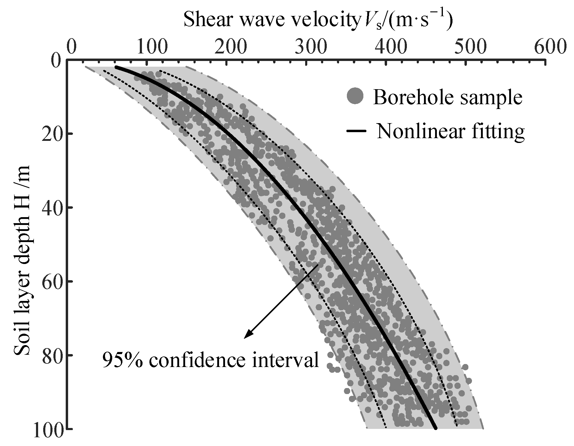
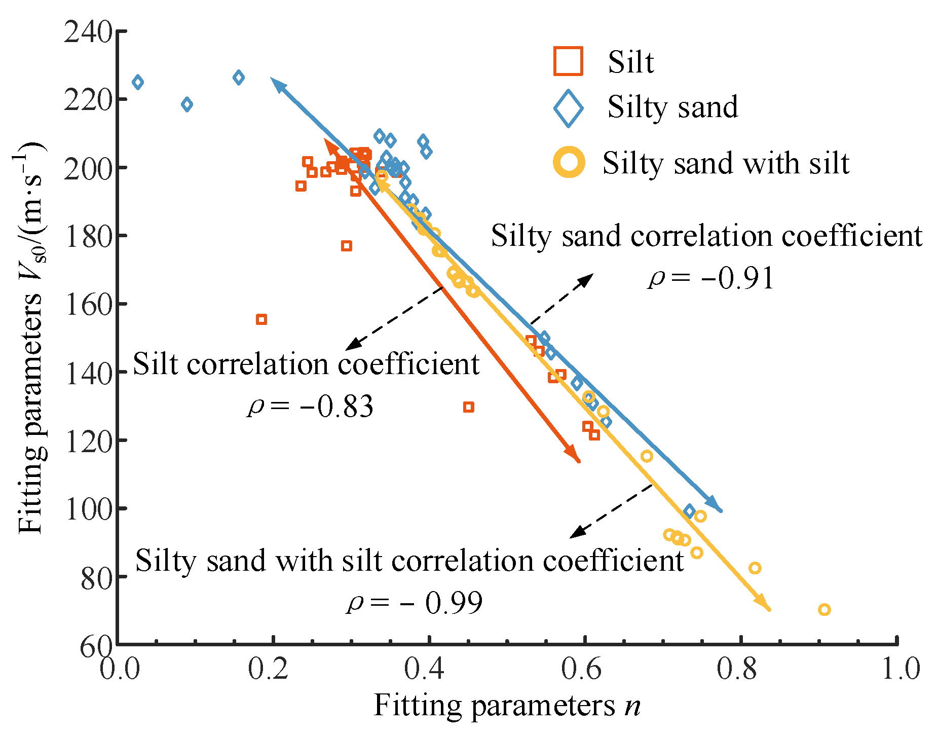
2.1. Trend Function and Its Uncertainty

2.1.1. Determination of Trend Functions

The correlation between shear wave velocity and burial depth, when modeled using an exponential function, meets the requirements of most engineering applications [48,49,50]. The nonlinear model employed in this paper is expressed as follows:
V s = V s 0 f h n
In the formula, f h = σ 0 / P a , where σ 0 = γ h ; Pa represents the standard atmospheric pressure, Pa = 100 kPa; σ 0 is the effective overburden pressure, which is directly related to the depth h; γ is the effective unit weight of the soil; Vs0 and n are fitting parameters, where Vs0 represents the shear wave velocity at σ 0 = 100 kPa, and n is associated with the soil’s coefficient of uniformity Cu [51,52]. In Equation (1), Vs0 is the shear wave velocity of the soil at σ 0 = 100 kPa (corresponding to a soil burial depth of approximately 10 m), meaning that Vs0 describes the shear wave velocity of the soil at a fixed depth. The two-dimensional random field illustrates the variability of soil parameters at different depths and various horizontal positions in space. Consequently, it is not feasible to directly utilize the two-dimensional random field to characterize the variability of Vs0, and in this paper, Vs0 is considered as a random variable. Equation (1) can be rewritten as follows:
V s / V s 0 = σ 0 / P a n
Equation (2) shows that the variable on the left side is related to shear wave velocity, which varies with both depth and horizontal position. If the variability of the effective unit weight of the soil is ignored, the factor σ 0 / P a on the right side depends only on burial depth. Therefore, the fitting parameter n must vary with both depth and horizontal position. This paper models the spatial variability of n using a random field.

2.1.2. Solution for the Mean and Standard Deviation of Soil Vs Varying with h

Using the point estimation method, we calculate the mean and standard deviation of Vs as a function of depth h when Equation (1) is the trend function [41]. First, Equation (1) is used to successively fit the relationship between the Vs of a certain type of soil and the dimensionless effective confining pressure σ 0 / P for each borehole at the collected sites. We then calculate the mean values V ¯ s 0 and n ¯ , as well as the standard deviations σ V s 0 and σ n for the fitting parameters Vs0 and n of that type of soil. The mean E[Vs(h)] of Vs for that type of soil at different depths can be calculated as follows:
E V s ( h ) = p + + V s + + + p + V s + + p + V s + + p V s
In the given context, the weighting functions are defined as follows: p++ = p−− = 1/4(1 + ρ), p+− = p−+ = 1/4 (1 − ρ). The correlation coefficient ρ for the parameters Vs0 and n is:
ρ = C O V V s 0 , n V V s 0 V n
In the formula, COV(Vs0,n) represents the covariance between Vs0 and n; V[Vs0] and V[n] are the variances of Vs0 and n, respectively. The term V s ± ± is defined as follows:
V s ± ± = V s 0 ¯ ± σ V s 0 f h n ¯ ± σ n
The standard deviation of Vs for soil at different depths h, denoted as σ V s h , is as follows:
σ V s h = E V s 2 E V s h 2
In the formula, E V s 2 denotes the second moment of Vs:
E V s 2 = p + + V s + + 2 + p + V s + 2 + p + V s + 2 + p V s 2
Through Equations (3)–(7), the mean and standard deviation of Vs for this type of soil at different depths h are obtained.
As indicated by Equation (4), this study accounts for the correlation of parameters within the trend function when analyzing the uncertainty of predictions derived from nonlinear trend functions. In contrast, previous research has not addressed this correlation [29,39,53].

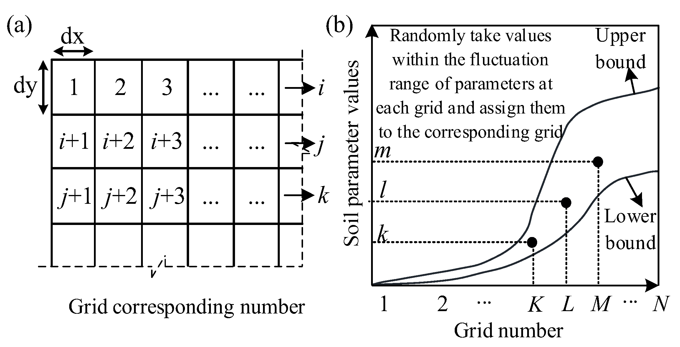
2.2. Simulation of the Random Vs-Structure Field

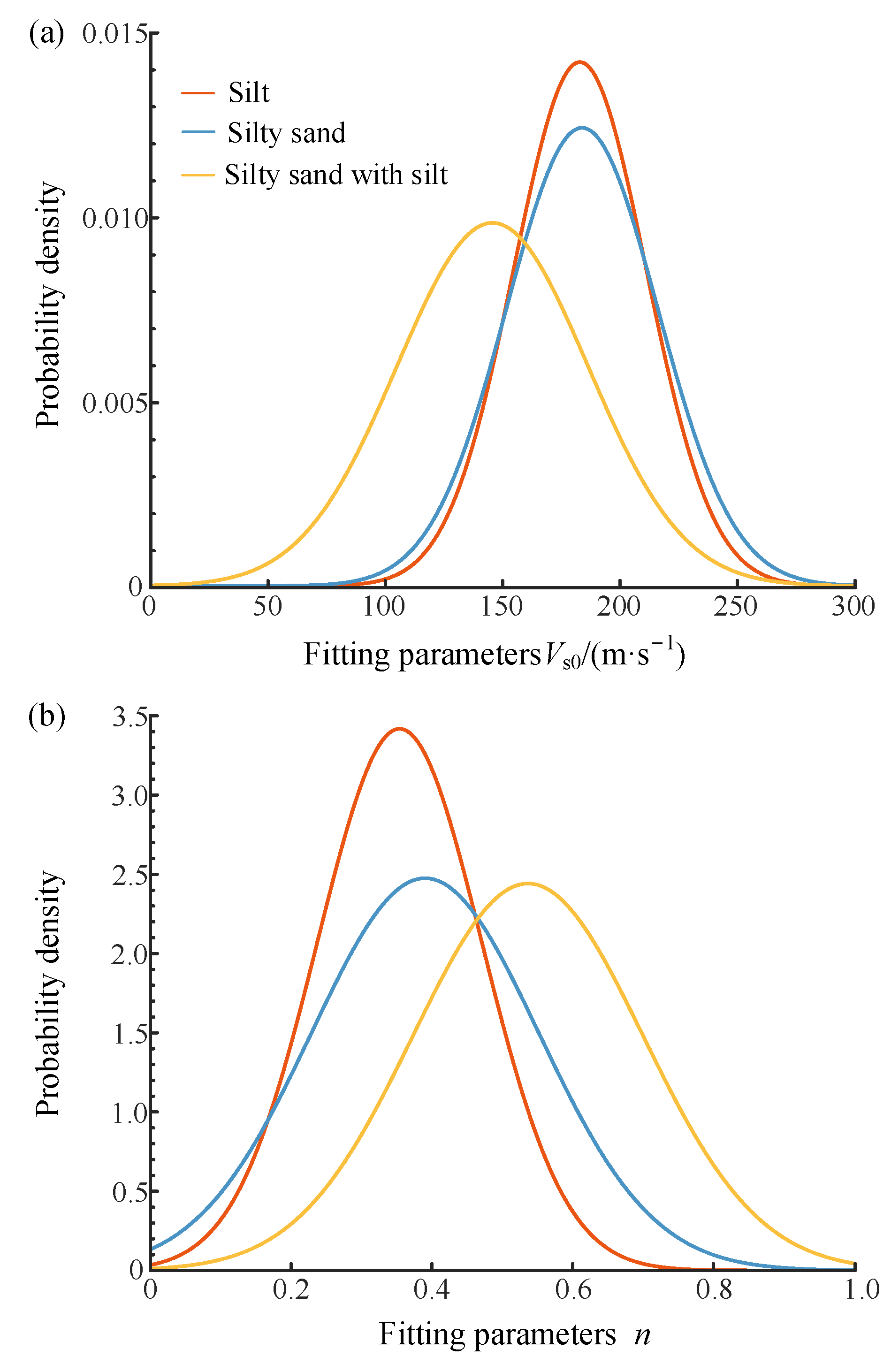
2.2.1. Simulating the Variability of Parameter Vs0 Using Random Variables

Clearly, Vs0 in Equation (2) is non-negative, and this paper employs a log-normal distribution to characterize the variability of Vs0. The statistical properties of Vs0 are transformed using a log-normal distribution as follows:
σ ln V = ln [ 1 + ( σ V / μ V ) 2 ]
μ ln V = ln μ V 1 2 σ V 2
where μv and σv represent the mean and standard deviation of Vs0, respectively, while μlnV and σlnV denote the mean and standard deviation of the logarithm of Vs0. An independent standard normal random sample matrix X is generated, and Vs0 can be calculated using the following equation:
V s 0 = exp ( μ ln V + σ ln V X )

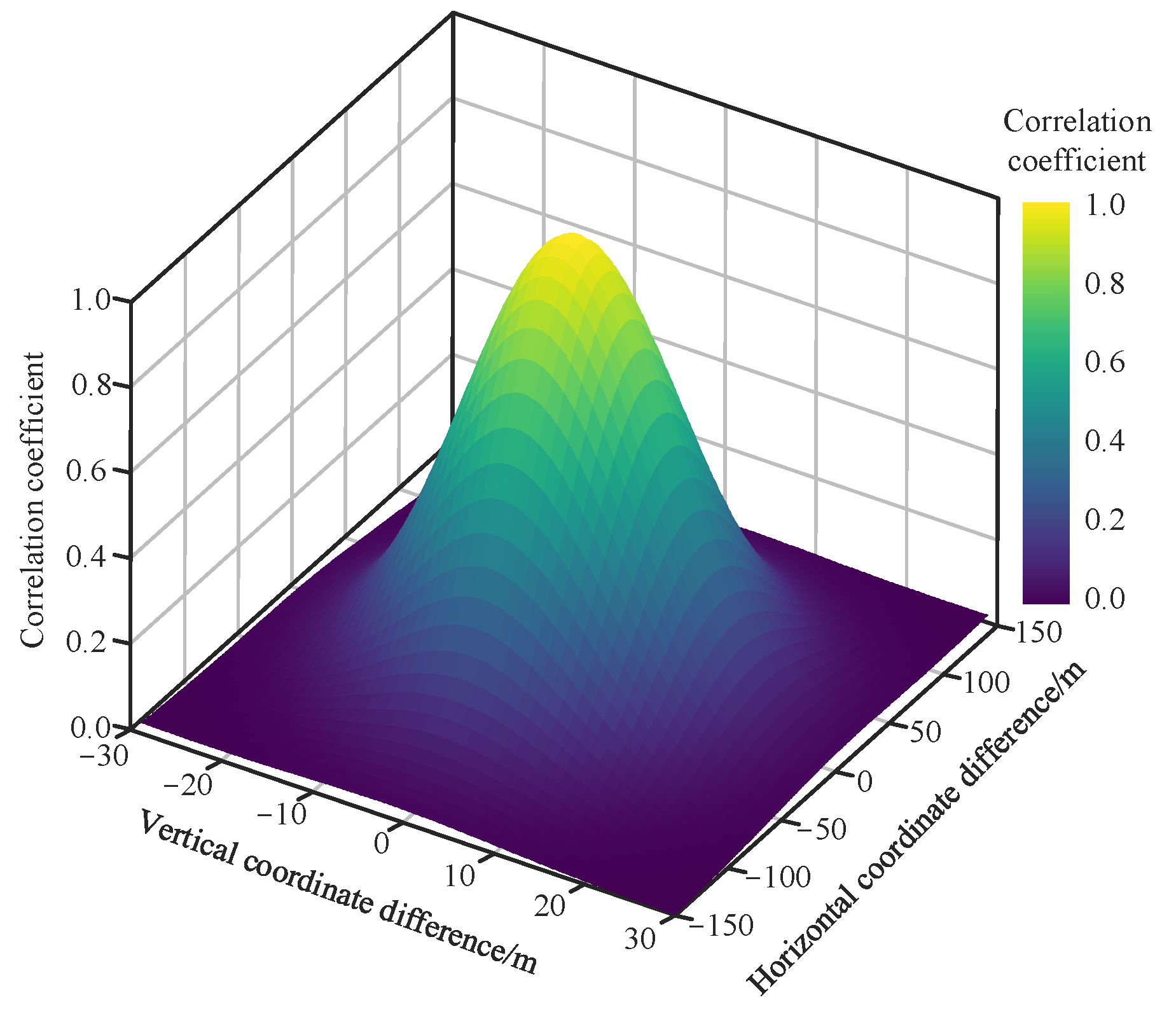
2.2.2. Simulating the Variability of Parameter n Using a Stationary Random Field

Next, a stationary random field is generated to fit the parameter n as described in Equation (2) [54]. An appropriate autocorrelation function is selected to characterize the spatial correlation of n. This paper employs a two-dimensional exponential autocorrelation function [33,39]:
R c , d = exp [ 2 ( | x c x d | δ x + | y c y d | δ y ) ]
where Rc,d represents the autocorrelation coefficient between positions c and d in the autocorrelation matrix R; the coordinates of positions c and d are (xc,yc) and (xd,yd), respectively; δx and δy denote the correlation distances in the horizontal and vertical directions, respectively. These distances reflect the strength of the autocorrelation of n in the horizontal and depth directions within a certain distance. As illustrated in Figure 2, when the two coordinates are within a certain distance, the autocorrelation of n decreases as the distance increases. Once beyond a certain range, it can be considered that the values of n at the two coordinate points are uncorrelated.
Generate an independent standard normal random sample matrix Y, and using Equation (12) with the Kaiser–Dickman algorithm, establish the relationship between Y and X to obtain a sample matrix U that considers the correlation between Y and X [44]:
U = ρ X + 1 ρ 2 Y
By performing a Cholesky decomposition, the correlation matrix R can be transformed into the product of a lower triangular matrix L and its transpose LT, that is, R = LLT. The correlated standard Gaussian random field lnH can be represented as:
ln H = L U
Typically, n is non-negative [51,52]. This paper simulates the spatial variability of n using a log-normal distributed random field. Furthermore, it is necessary to transform the statistical information of n using a log-normal distribution transformation.
σ ln n = ln [ 1 + ( σ n / μ n ) 2 ]
μ ln n = ln μ n 1 2 σ ln n 2
where μn and σn are the mean and standard deviation of n, respectively. μ ln n and σ ln n are the mean and standard deviation of the logarithm of n, respectively. The log-normal random field H for n can be expressed as:
H = exp ( μ ln n + σ ln n ln H )
By using Equations (12)–(16), the simulation of the random field for n can be completed.

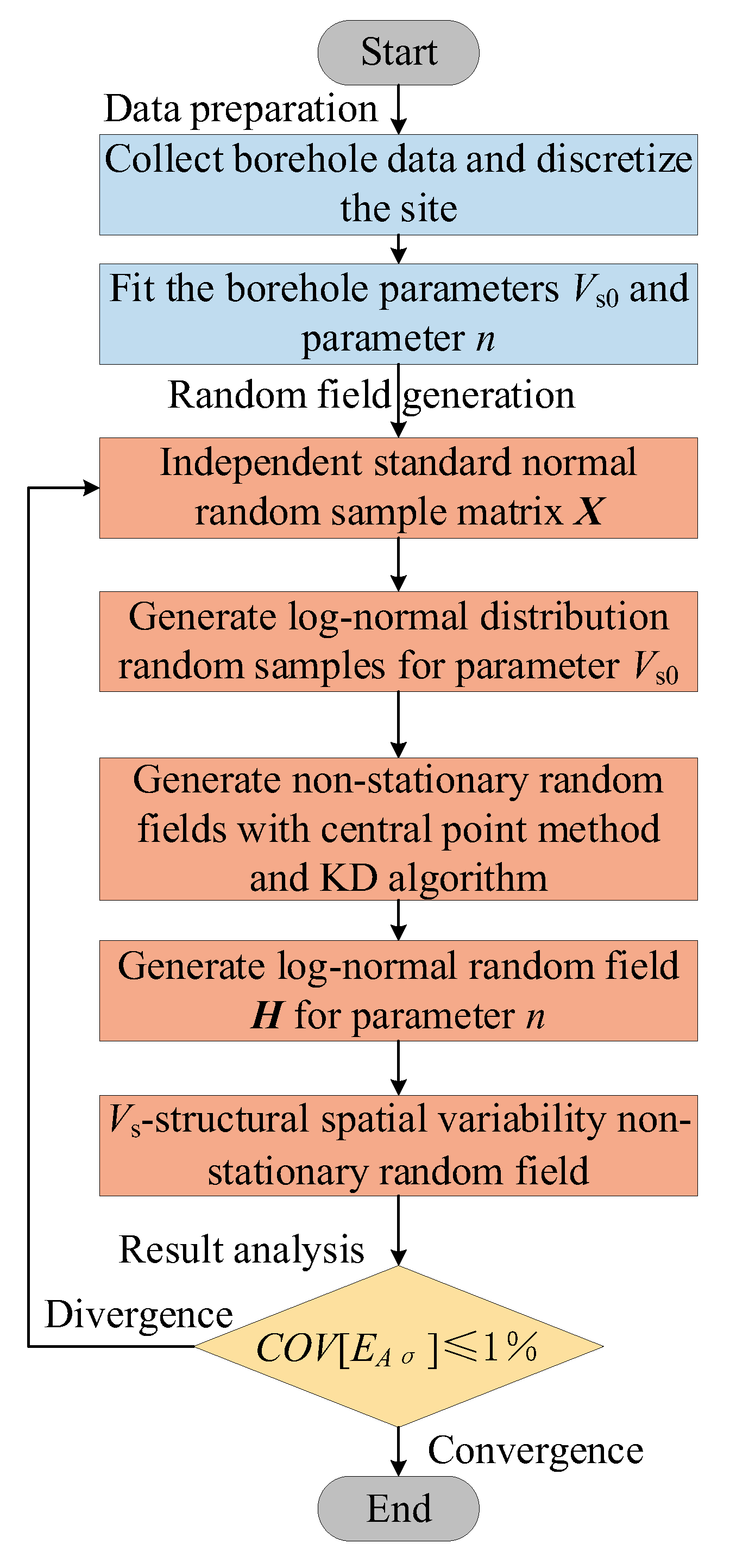
2.2.3. Acquisition of the Random Vs-Structure Non-Stationary Random Field

The value of n given by Equation (16) takes into account the correlation between n and Vs0. By substituting the values of Vs0 and n obtained from Equations (10) and (16) into Equation (2), respectively, one can obtain a non-stationary random field that describes the spatial variability of the Vs-structure.

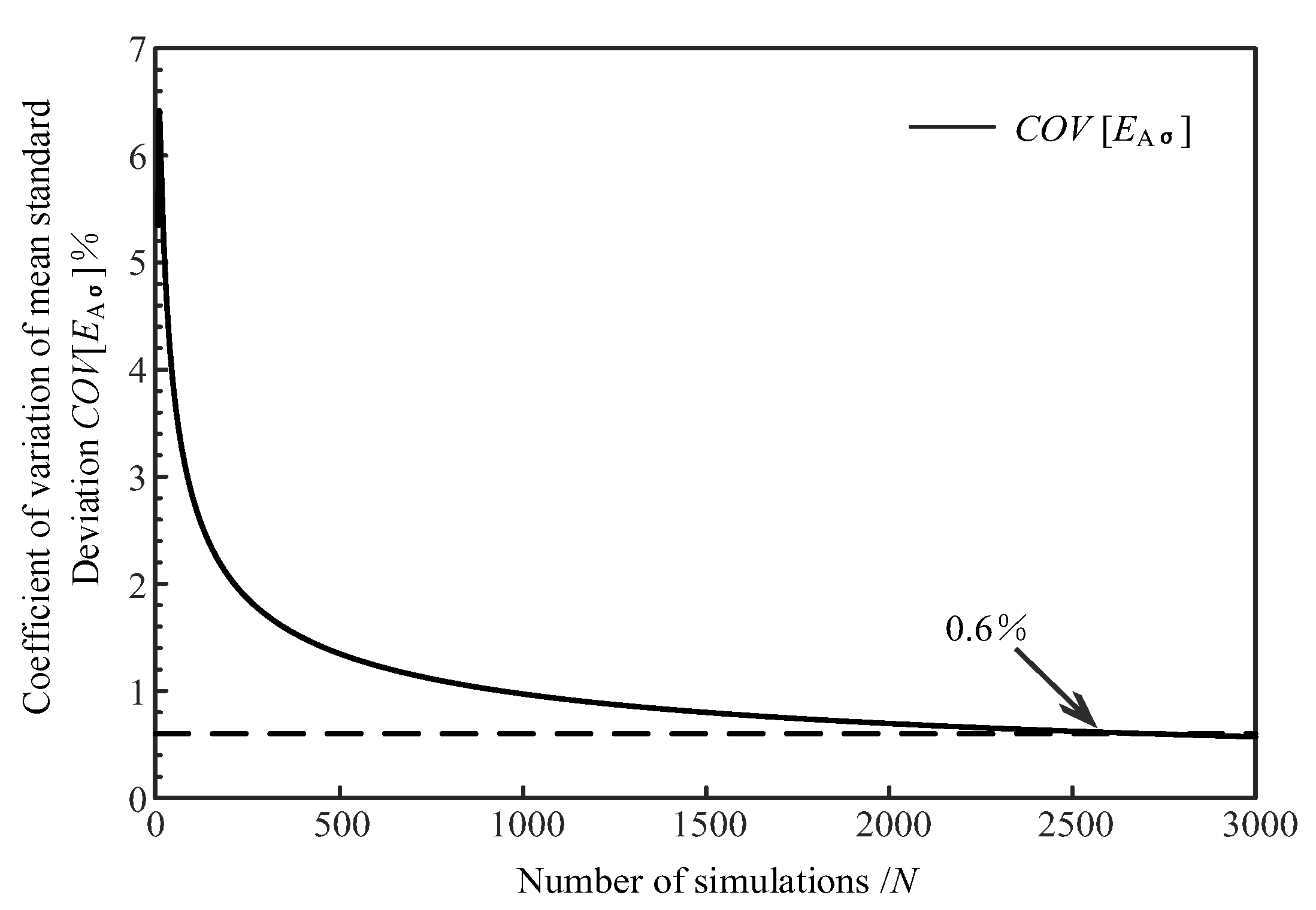
2.3. Determining the Number of Simulations N for the Random Field

To ensure that the simulation covers various conditions of geotechnical parameters at the site, a sufficient number of simulations must be conducted. However, conducting an excessive number of simulations may lead to overconsumption of computational resources and a significant decrease in efficiency. When the spatial variability of the random Vs-structure converges and is within a certain fixed range, it can be considered that the simulation has achieved statistical stability. This criterion is used to determine the number of simulations N. For the l-th (l = 1, 2, …, N) random field simulation, the standard deviation of a grid point uα at a certain location on the site is given by [34]:
σ V s u α = l = 1 N V s l u α l = 1 N V s l u α / N 2 / N 1
where V s l u α represents the simulated value of Vs at the grid point uα during the l-th random simulation. After N simulations, the mean value EAσ of all grid points on the site is:
E A σ = 1 n α = 1 n σ V s u α
where n is the total number of grids on the site, representing the size of the site. Different values of N will yield different EAσ, and subsequently, the coefficient of variation COV[EAσ] can be calculated. When the coefficient of variation COV[EAσ] converges and the convergence value is less than or equal to 1%, it is considered that N simulations can provide a comprehensive distribution of the possibilities for the random Vs-structure [34]. Figure 3 illustrates the process of simulating the non-stationary random field of shear wave velocity Vs-structure in this paper.

3. Results

3.1. Location of the Study Area

Before simulating the geotechnical parameters, it is necessary to fully assess the site scale and the corresponding grid size to ensure the accuracy and effectiveness of the simulation. The relative elevation is established based on the ground level, and the simulation boundary is determined according to the deepest existing borehole data, with a maximum depth of 100 m. The horizontal scale is based on the distance between the two farthest boreholes on the site, set at 500 m. Therefore, the scale of the simulation site is set to a horizontal distance of 500 m and a depth of 100 m. The site uses a ZD16 borehole shear wave velocity tester for in situ measurements [55,56]. Dynamic excitation testing provides accurate shear wave velocity data, allowing for analysis of geological structures and material properties and offering reliable wave velocity parameters for geological and engineering applications. Table 1 below provides information on the relevant geotechnical parameters at the site.

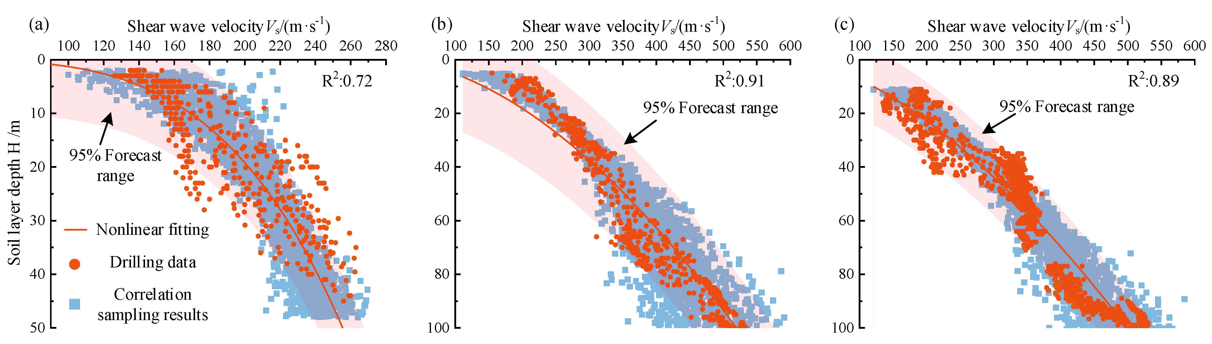
3.2. Statistical Characteristics of Measured Vs Data

Figure 4 presents the relationship between the Vs values of the soil in the study area and the depth h. From Figure 4, it can be observed that the overall characteristic of the shear wave velocity of the soil increases with increasing depth, and there is a significant nonlinear relationship between the two. Additionally, the variability of the Vs values also increases with depth (Figure 4 does not distinguish between soil types). Figure 5 shows the standard penetration blow count, a parameter representing soil strength, corresponding to the shear wave velocity. It can be observed from Figure 4 that the blow count increases in variability with depth, consistent with the structure of the shear wave velocity. Figure 6, on the other hand, illustrates the correlation between the parameters n and Vs0 for different types of soil in the study area. It is evident from Figure 6 that there is a clear negative correlation between n and Vs0 for all types of soil. Therefore, it is quite reasonable to consider the nonlinear relationship of soil Vs with depth h and the correlation between n and Vs0 when describing the spatial variability of Vs, as proposed in Section 2 of this paper.
Figure 6 indicates that in the dual-parameter fitting results of the existing borehole data from a certain area in Jiangsu, the fitting parameters Vs0 and n exhibit a strong negative correlation. Under different stratigraphic conditions, sampling results that are consistent with the intercorrelation of the two fitting parameters from the borehole samples can be obtained.

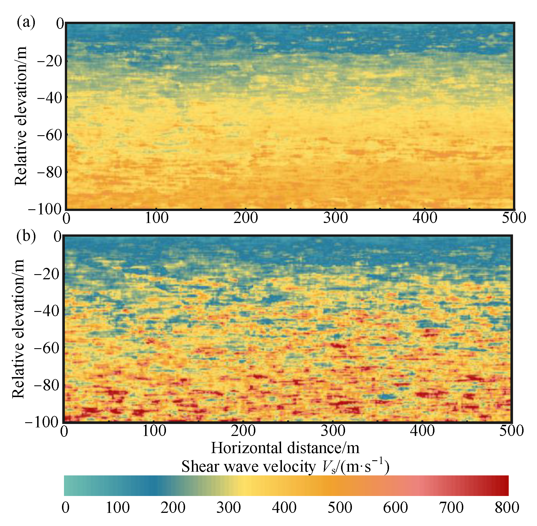
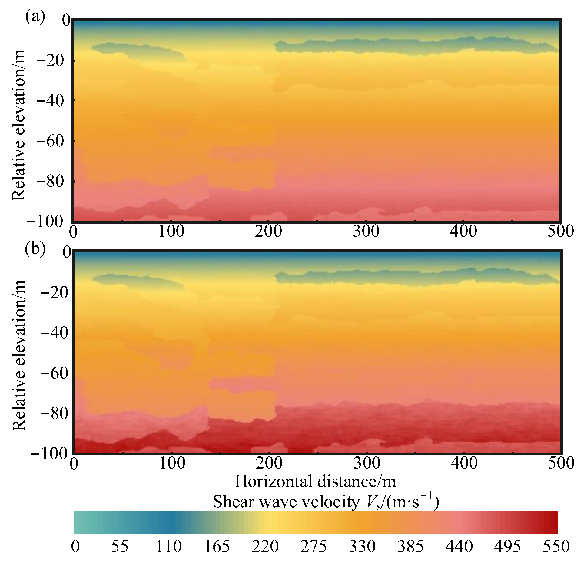
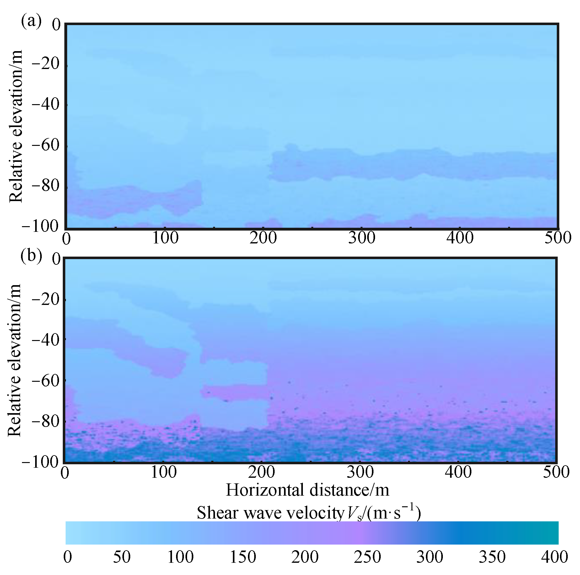
3.3. Simulation of the Non-Stationary Vs-Structure Random Field in the Study Area

Based on the principles of random field simulation and the existing borehole data in the study area, a non-stationary random field simulation of the Vs-structure for this region is conducted. Prior to the simulation, the site is discretized using an appropriately sized grid. When setting the grid size, to avoid discontinuity and inconsistency in the simulation results within the same grid, it is essential to ensure that its dimensions in both the horizontal and vertical directions do not exceed the thickness of the thinnest stratum. According to the measured results from the boreholes in the study area, the grid size is set to 2 m horizontally and 0.5 m in the vertical direction. There is a significant difference in the spatial autocorrelation of geotechnical parameters in the horizontal and vertical directions. The fluctuation scale in the horizontal direction is much greater than in the vertical direction. Referring to the commonly used values for the horizontal and vertical correlation distances of geotechnical parameters provided by Phoon K.K., this paper sets the autocorrelation distances for the site in the horizontal and longitudinal directions to 20 m and 2 m, respectively [57].
Figure 7 presents the marginal probability density curves for the parameters Vs0 and n corresponding to different soil types in the study area. After the Kolmogorov–Smirnov test, it has been determined that Vs0 and n for all types of soil in the study area follow normal and log-normal distributions, respectively.
Utilizing the methods described in Section 2, after conducting multiple simulations, the average coefficient of variation of the standard deviation for the site is calculated. As shown in Figure 8, after 3000 simulations, COV[EAσ] converges and is less than 1%. Therefore, this paper sets the number of simulations N to 3000.
As shown in Figure 9, after conducting 3000 simulations, to represent the comprehensive situation of the simulation, the mean and standard deviation of the 3000 sampled values at each grid point uα are calculated to express its overall statistical characteristics.
Figure 10a presents a typical result obtained from simulating the random Vs-structure of the study area using the method proposed in Section 2 of this paper, where the correlation coefficient ρ in Equation (12) is taken as the true value calculated from the actual measured data (i.e., considering the real correlation between Vs0 and n). Figure 10b presents a typical result obtained from simulating the random Vs-structure of the study area by using the method proposed in Section 2 of this paper, where the correlation coefficient ρ in Equation (12) is set to 0 (i.e., not considering the correlation between Vs0 and n). Both results overall show a trend of increasing Vs with increasing depth h.
Comparing Figure 10a,b, when the correlation between Vs0 and n is not considered, the spatial autocorrelation of the Vs-structure is significantly weakened. Lower simulated values frequently appear around high simulated values, especially below 50 m depth.
To demonstrate the impact of the two sampling methods on the spatial autocorrelation of the final Vs parameters, the local Moran’s index is introduced to represent the strength of autocorrelation of the parameters at different spatial locations. The local Moran’s index Ii at the center of each grid is:
I i = V s u i V s ¯ j = 1 n ω i j V s u j V s ¯ i = 1 n V s u i V s ¯ 2
where V s u i and V s u j represent the simulated Vs values at grid positions ui and uj, respectively; V s ¯ is the mean of the simulated Vs results in the study area; ωij is an element of the spatial weight matrix based on the spatial distance between adjacent points, calculated as the reciprocal of the distance between the two points. The local Moran’s index can be considered as the ratio of the covariance to the variance between geotechnical parameter values in adjacent spaces. As shown in Figure 11, this index can be used to identify areas where high and low values of parameters aggregate. When the local Moran’s index is positive and has a larger value, it indicates that the spatial autocorrelation of shear wave velocity Vs in that area is stronger. Conversely, it indicates negative autocorrelation. From Figure 11, it can be seen that when considering the cross-correlation between Vs0 and n, the low and high values of Vs results aggregate in the shallow and deep layers of the simulated site, respectively, and the negative correlation areas are mainly concentrated between the shallow and deep layers, with weak negative correlation. When not considering the cross-correlation between Vs0 and n, the simulated results of the Vs-structure show areas of high and low abnormal value aggregation and interspersed high and low value aggregation areas in the deep layers, indicating that there is no significant spatial correlation between the parameter values in that area.
Figure 12 and Figure 13 show the mean and standard deviation of Vs0 values at different locations in the study area obtained after 3000 simulations, with and without considering the correlation between Vs0 and n, respectively. When considering the correlation between Vs0 and n, the mean Vs values in the 80–100 m depth range of the study area are significantly lower than the corresponding mean Vs values in the same depth range when not considering the correlation between Vs0 and n.
When considering the correlation between Vs0 and n, the standard deviation of Vs in the 80–100 m depth range of the study area is also significantly lower than the standard deviation of Vs in the corresponding depth range when not considering the correlation between Vs0 and n.
Regardless of whether the correlation between Vs0 and n is considered, overall, the mean of the simulated Vs-structure results in the study area increases with the increase in h, following the pattern that the shear wave velocity Vs gradually increases as sediments are compacted under their own weight. The standard deviation of the simulated Vs-structure results in the study area varies with h, corroborating the non-stationary characteristic that the variability of geotechnical parameters, which are significantly influenced by overburden pressure, changes with h [16,17,18].

4. Discussion

4.1. Liquefaction Discriminant Method for Soil Based on Shear Wave Velocity

This paper applies the liquefaction discrimination method based on shear wave velocity, as outlined by Chen et al. (2019), to evaluate the probability of soil liquefaction in the study area, considering the spatial variability of the Vs-structure [6]. The cyclic stress ratio (CSR) is normalized to the cyclic stress ratio corresponding to a seismic moment magnitude Mw = 7.5 and an overburden effective pressure σ v = 100 kPa , with the calculation formula for C S R M w = 7.5 , σ v = 100 kPa being:
C S R M w = 7.5 , σ v = 100 kPa = 0.65 σ v σ v a max g γ d 1 M S F 1 K σ
where σv is the total overburden stress at the soil layer depth z; σ v is the effective overburden stress at the soil layer depth z; amax is the peak horizontal ground acceleration, with the unit g; g is the acceleration due to gravity, g = 9.8 m/s2; γd is the shear stress reduction coefficient for the soil layer; MSF is the magnitude scaling factor; and Kσ is the correction coefficient for effective overburden pressure. The γd at depth z is calculated as follows:
γ d = exp [ α ( h ) + β ( h ) M W ] α ( z ) = 1.012 1.126 sin z 11.73 + 5.133 β ( z ) = 0.106 + 0.118 sin z 11.28 + 5.142
The calculation formulas for the remaining correction coefficients MSF, Kσ, and Cσ are as follows:
M S F = 6.9 exp ( M W / 4 ) 0.058 K σ = 1 C σ ln ( σ v / P a ) C σ = 1 18.9 2.55 ( N 1 ) 60 c s
where σ v and Pa have the same units; (N1)60CS is the corrected SPT blow count for equivalent clean sand; and Cσ is the correction parameter for calculating Kσ.
The cyclic resistance ratio C R R M W = 7.5 , σ v = 100 kPa based on the shear wave velocity Vs parameter under seismic action, with moment magnitude MW = 7.5 and effective overburden pressure σ v = 100 kPa as the baseline, is expressed as follows:
C R R M W = 7.5 , σ v = 100 kPa = exp V s 1 86.4 + V s 1 134.0 2 V s 1 125.2 3 + V s 1 158.5 4 4.8
where Vs1 is the adjusted shear wave velocity, and the following equation is the calculation formula for it:
V s 1 = V s P a σ v 0.25
In this paper, the spatial variability of the peak ground acceleration at the surface is not considered. According to the seismic parameter zoning map of China, the peak ground acceleration amax for the surrounding area with a probability of exceedance of 10% within 50 years is 0.2 g. To fully assess the liquefaction potential of the soil in the study area under the influence of earthquakes, the peak ground acceleration at the surface of this stratum is uniformly taken as 0.2 g. The liquefaction potential of the soil at each grid point uα can be represented by the safety factor Fs:
F s = C R R M W = 7.5 , σ v = 100 kPa C S R M W = 7.5 , σ v = 100 kPa
In the formula, liquefaction occurs only when Fs ≤ 1. The liquefaction probability PL(uα) at each location can be calculated as follows:
P L ( u α ) = N ( F s 1 ) N
where N(Fs ≤ 1) represents the number of times Fs ≤ 1 calculated using the Vs values obtained from the random field simulation results.

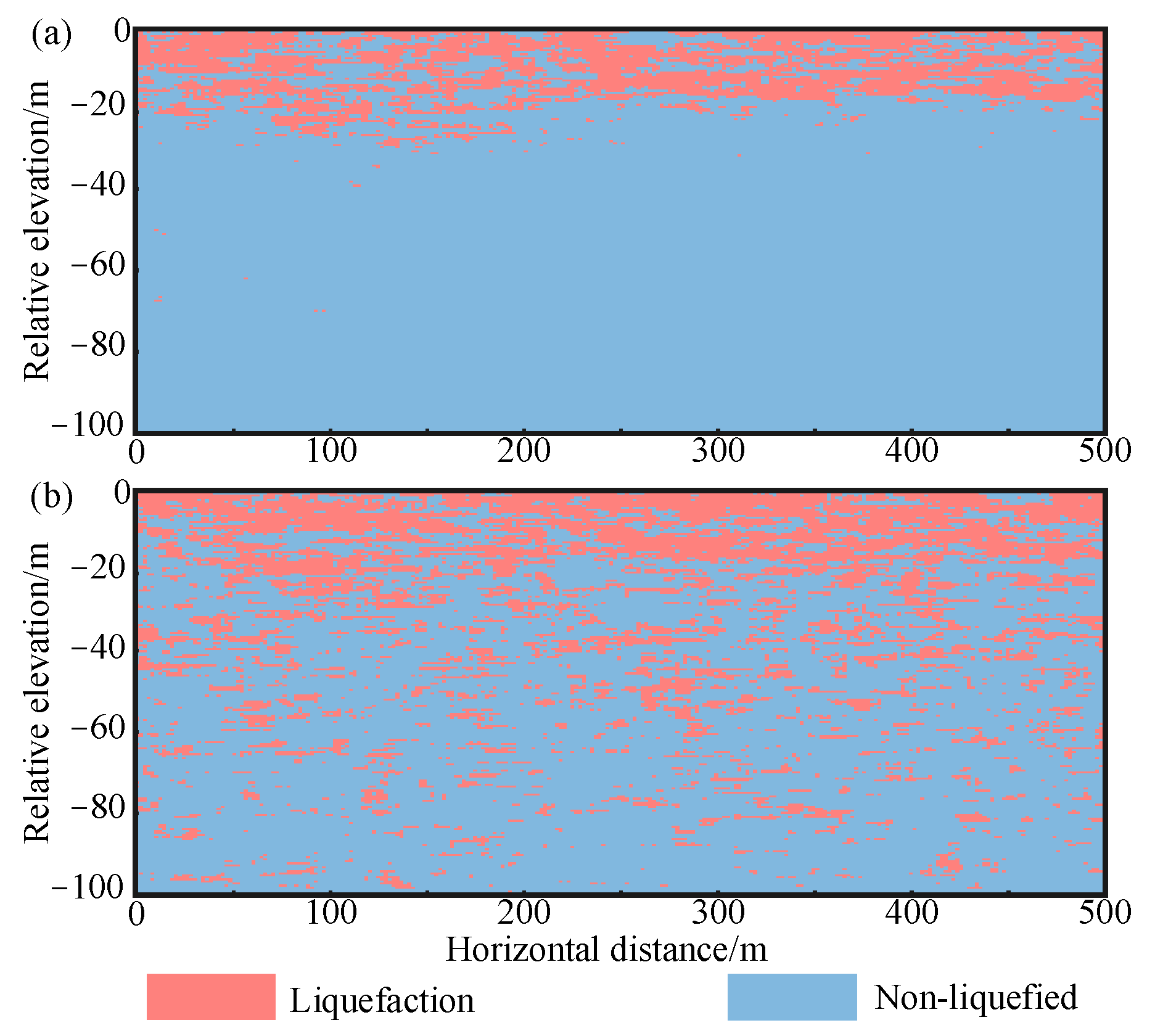
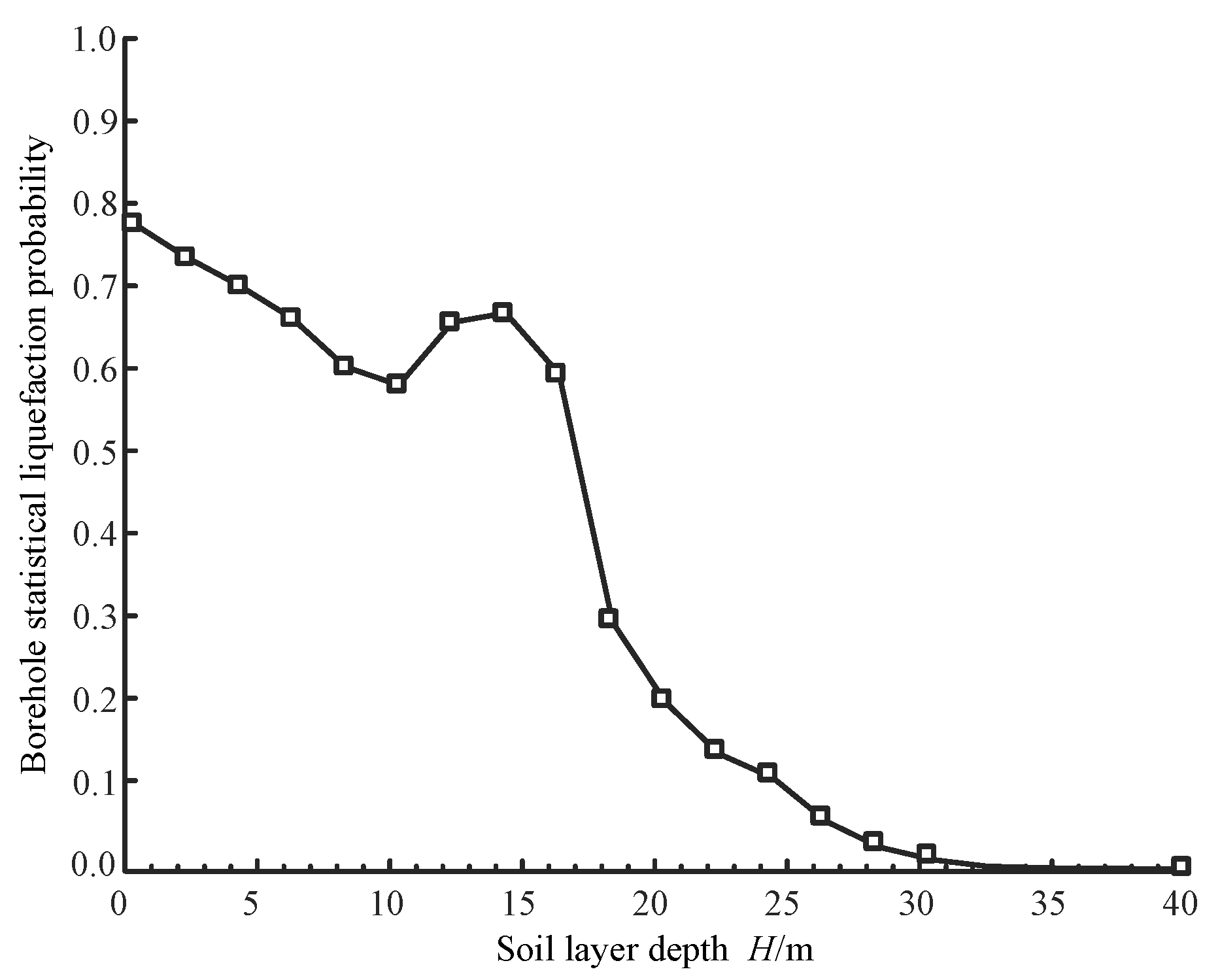
4.2. Liquefaction Discriminant Results in the Study Area

By substituting the possible Vs-structure of the study area considering the correlation between Vs0 and n as shown in Figure 10a and the possible Vs-structure without considering the correlation between Vs0 and n as shown in Figure 10b into the liquefaction discrimination process described in Section 4.1, the corresponding liquefaction discrimination results for the study area are obtained, as illustrated in Figure 14a,b. When considering the correlation between Vs0 and n, the liquefiable areas in the study area are concentrated in the region shallower than 30 m; when not considering the correlation between Vs0 and n, although the liquefiable areas are also densely distributed shallower than 30 m, sporadic distributions of liquefiable areas are also present deeper than 30 m. It is evident that not considering the correlation between Vs0 and n may overestimate the liquefaction potential of the soil in the study area.
Figure 15 presents the liquefaction probabilities at any location in the study area calculated using Equation (26) after inputting the distribution results of the Vs-structure obtained from 3000 simulations into the liquefaction discrimination process described in Section 4.1. When considering the correlation between Vs0 and n, the areas with higher liquefaction probabilities in the study area are mainly distributed within 40 m depth, with liquefaction probabilities basically below 0.1 for depths greater than 40 m. When not considering the correlation between Vs0 and n, the liquefaction probabilities for soil deeper than 40 m in the study area range between 0.4 and 0.6, which is significantly higher than the liquefaction probabilities for the corresponding depth regions when considering the correlation between Vs0 and n. This further confirms that not accounting for the correlation between Vs0 and n can significantly overestimate the liquefaction potential of the soil in the study area.

4.3. Verification of Liquefaction Discriminant Accuracy

The random sampling methodology utilized in this study is based on geotechnical parameters derived from existing borehole data. Figure 16 illustrates the borehole data alongside the sampling results obtained using the approach described in Section 2. Analysis of the figure indicates that the velocity data points for shallow silt exhibit considerable scatter, resulting in a relatively broad sampling range. In contrast, the borehole velocity data for silty sand and silty sand with silt align closely with established geotechnical parameter trends, demonstrating an increase in shear wave velocity dispersion with depth. Additionally, the non-stationary random field sampling of the Vs-structure effectively captures the borehole shear wave velocity data, simulating a wide range of potential site conditions and providing robust data support for comprehensive site evaluation.
To verify the accuracy of the simulation results in this paper, the actual measured Vs data from 30 boreholes in the study area are used to perform liquefaction discrimination using the method described in Section 4.1. For any depth h, the Vs value at h provided by each borehole is substituted into the liquefaction discrimination process in Section 4.1 to calculate the liquefaction resistance safety factor Fs. The number of times Fs is less than 1, divided by 30, gives the liquefaction probability at that depth. This liquefaction probability is then compared with the results obtained from the liquefaction probability discrimination based on the Vs-structure non-stationary random field simulation results proposed in this paper. Figure 17 shows the liquefaction probabilities at different depths obtained from the liquefaction discrimination using the Vs data revealed by the actual boreholes in the study area. As shown in Figure 17, the liquefaction areas identified by the Vs values revealed by the actual boreholes are mainly distributed within 40 m depth, and the liquefaction probabilities are all 0 below 40 m depth. This is consistent with the results obtained from the liquefaction probability discrimination using the Vs values from the non-stationary random field simulation considering the correlation between Vs0 and n, proving the rationality of the method proposed in this paper.

5. Conclusions

This paper proposes a non-stationary random field model that effectively simulates the spatial variability of soil parameters significantly influenced by the overburden pressure. By using a power function Vs = Vs0[f(h)]n to describe the nonlinear variation of shear wave velocity Vs with depth h and performing a fitting analysis of measured borehole data, a significant correlation between the parameters Vs0 and n is observed. Therefore, when simulating the variability of Vs, the correlation between these two parameters must be taken into account. Further analysis of their physical meaning shows that Vs0 and n should be described using a random variable model and a stationary random field model, respectively, to construct a non-stationary random field model that characterizes the variation of Vs with depth.
To validate the effectiveness of this model, a random Vs-structure for a seabed in China was simulated, and the liquefaction probability of the seabed was assessed based on the simulation results. The results indicate that the proposed method can accurately simulate the nonlinear trend and non-stationary characteristics of soil Vs with depth, with the liquefaction probability closely matching field measurements, thereby verifying the model’s reliability. Additionally, this study finds that the correlation between Vs0 and n significantly affects the simulation results. Ignoring this correlation broadens the sampling range, leading to a substantial increase in the variability of the simulated Vs in the study area. Thus, the correlation between these two parameters must be fully considered to improve simulation accuracy in similar studies.
Geotechnical strength-related parameters typically exhibit a nonlinear trend due to complex stratigraphic deposition conditions and show spatial correlation between fitted parameters, which significantly impacts site simulation results. The non-stationary random field model proposed in this paper effectively addresses this issue. This method is not only suitable for simulating the spatial variability of soil shear wave velocity Vs but also applicable to a range of soil parameters significantly influenced by overburden pressure.

Author Contributions

Conceptualization, Z.Z. (Zhengyang Zhang), G.X., Y.Z., J.H. and Z.Z. (Zhenglong Zhou); formal analysis, F.P. and Y.Z.; funding acquisition, J.H.; investigation, Y.Z.; methodology, Y.Z.; supervision, Z.Z. (Zhenglong Zhou); validation, Z.Z. (Zhengyang Zhang) and G.X.; writing—original draft, Z.Z. (Zhengyang Zhang) and Y.Z.; writing—review and editing, G.X., F.P. and J.H. All authors have read and agreed to the published version of the manuscript.

Funding

This work was supported by the Natural Science Foundation of Xinjiang Uygur Autonomous Region (2024D01C243), Tianchi Talent Introduction Plan, Basic Research Funds for Universities in Xinjiang Uygur Autonomous Region Research Project (XJEDU2024P026), and the Sichuan Science and Technology Program (2024YFHZ0154), National Natural Science Foundation of China (52208349).

Institutional Review Board Statement

Not applicable.

Informed Consent Statement

Not applicable.

Data Availability Statement

The data presented in this study are available upon request from the corresponding author.

Conflicts of Interest

The authors declare no conflicts of interest.

Nomenclature

Notation
VsShear wave velocity
hDepth
σ 0 Effective overburden pressure
PaStandard atmospheric pressure
γ Effective unit weight of the soil
Vs0Shear wave velocity of the soil at a fixed depth
nAssociated with the soil’s coefficient of uniformity
V ¯ s 0 , n ¯ Mean values of Vs0, n
σ V s 0 , σ n Standard deviations of Vs0, n
E[Vs(h)]Mean values of Vs at different depths
p±±Weight function
ρCorrelation coefficient
E V s 2 The second-order moments of Vs
μv, σvMean and standard deviation of Vs0
μlnV, σlnVLog mean and standard deviation of Vs0
δx, δyAutocorrelation distances in the horizontal and vertical directions
RAutocorrelation coefficient matrix
USampling matrix
X, YStandardized positronic distribution sampling matrix
LCholesky’s decomposition of the lower triangular matrix
μlnn, σlnnLog mean and standard deviation of n
HLognormal random field
V s l u α Simulated values of Vs at grid point uα in the lth stochastic simulation
COV[E]Vs mean standard deviation coefficient of variation
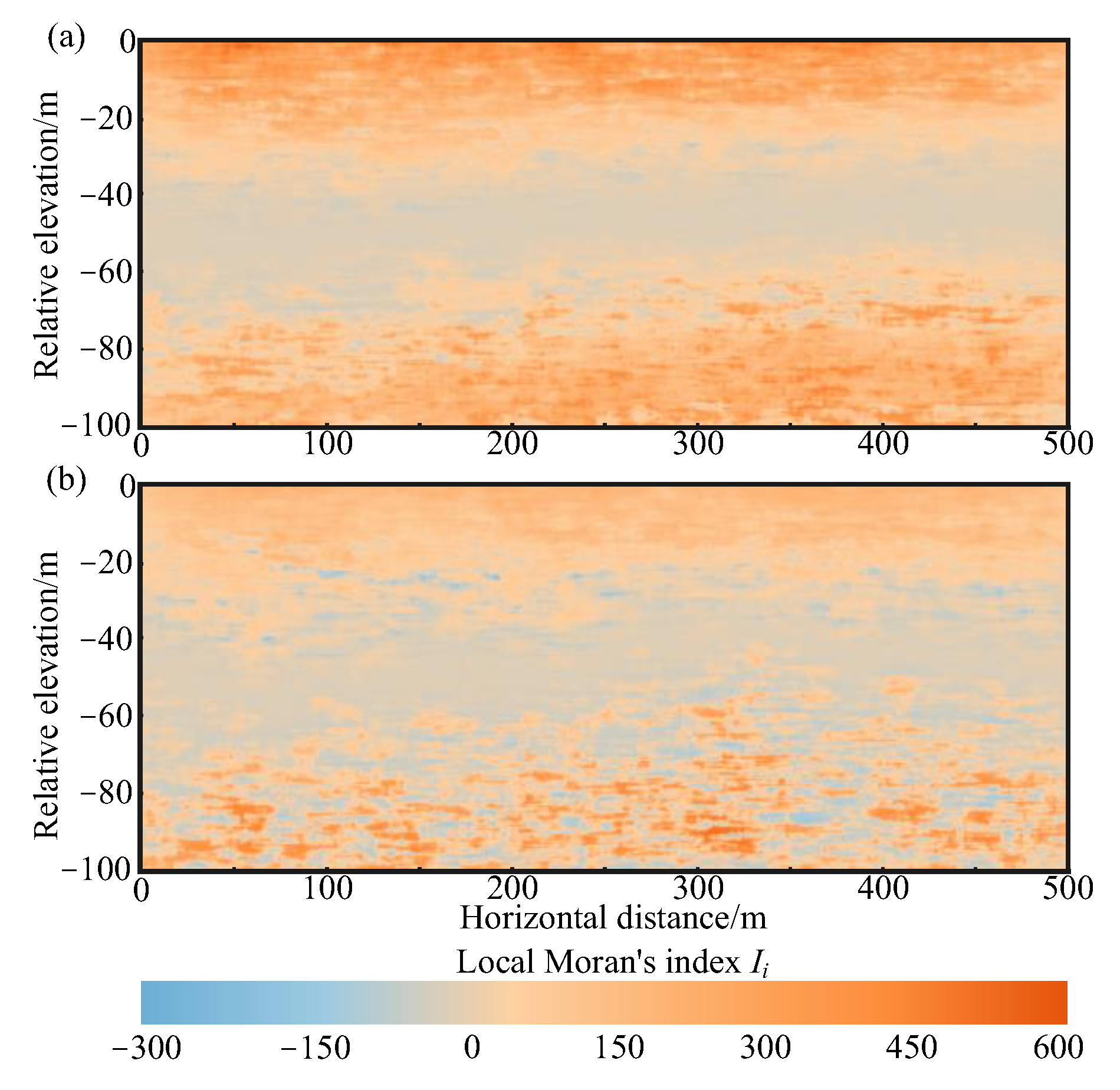
IiLocalized Moran index
σvSoil overburden pressure
σ v Effective soil overburden pressure
amaxPeak horizontal ground acceleration
gGravitational acceleration
γdSoil shear stress reduction factor
Kσ, CσEffective overburden pressure correction factor
α(z), β(z)Cyclic stress ratio depth correction factor
MSFMagnitude calibration factor
Vs1Modified shear wave velocity
FsFactor of safety for liquefaction potential of soils
PL(uα)Probability of soil liquefaction

References

  1. Zhang, Y.; Zhao, K.; Peng, Y.J.; Chen, G.X. Dynamic shear modulus and damping ratio characteristics of undisturbed marine soils in the Bohai Sea, China. Earthq. Eng. Eng. Vib. 2022, 21, 297–312. [Google Scholar] [CrossRef]
  2. Bhattacharya, S.; Hyodo, M.; Goda, K.; Tazoh, T.; Taylor, C.A. Liquefaction of soil in the Tokyo Bay area from the 2011 Tohoku (Japan) earthquake. Soil Dyn. Earthq. Eng. 2011, 31, 1618–1628. [Google Scholar] [CrossRef]
  3. Orense, R.P.; Pender, M.J.; Wotherspoon, L.M. Analysis of soil liquefaction during the recent Canterbury (New Zealand) earthquakes. Geotech. Eng. J. Seags Agssea 2012, 43, 8–17. [Google Scholar]
  4. Sonmez, B.; Ulusay, R. Liquefaction potential at Izmit Bay: Comparison of predicted and observed soil liquefaction during the Kocaeli earthquake. Bull. Eng. Geol. Environ. 2008, 67, 1–9. [Google Scholar] [CrossRef]
  5. Andrus, R.D.; Stokoe II, K.H. Liquefaction resistance of soils from shear-wave velocity. J. Geotech. Geoenviron. 2000, 126, 1015–1025. [Google Scholar] [CrossRef]
  6. Chen, G.X.; Kong, M.Y.; Khoshnevisan, S.; Chen, W.Y.; Li, X.J. Calibration of Vs-based empirical models for assessing soil liquefaction potential using expanded database. Bull. Eng. Geol. Environ. 2019, 78, 945–957. [Google Scholar] [CrossRef]
  7. Liu, W.X.; Juang, C.H.; Chen, Q.S.; Chen, G.X. Dynamic site response analysis in the face of uncertainty–an approach based on response surface method. Int. J. Numer. Anal. Met. 2021, 45, 1854–1867. [Google Scholar] [CrossRef]
  8. Al-Jeznawi, D.; Sadik, L.; Al-Janabi, M.A.Q.; Alzabeebee, S.; Hajjat, J.; Keawsawasvong, S. Developing Vs-NSPT Prediction Models Using Bayesian Framework. Transp. Infrastruct. Geotechnol. 2024, 11, 1777–1798. [Google Scholar] [CrossRef]
  9. Esfehanizadeh, M.; Nabizadeh, F.; Yazarloo, R. Correlation between standard penetration (NSPT) and shear wave velocity (VS) for young coastal sands of the Caspian Sea. Arab. J. Geosci. 2015, 8, 7333–7341. [Google Scholar] [CrossRef]
  10. Hossain, M.B.; Rahman, M.M.; Haque, M.R. Empirical correlation between shear wave velocity (Vs) and uncorrected standard penetration resistance (SPT-N) for Dinajpur District, Bangladesh. J. Nat. 2021, 3, 25–29. [Google Scholar] [CrossRef]
  11. Kishida, T.; Tsai, C. Prediction Model of Shear Wave Velocity by Using SPT Blow Counts Based on the Conditional Probability Framework. J. Geotech. Geoenviron. 2017, 143, 4016108. [Google Scholar] [CrossRef]
  12. Dobry, R.; Abdoun, T.; Stokoe, K.H.; Moss, R.E.S.; Hatton, M.; El, G.H. Liquefaction Potential of Recent Fills versus Natural Sands Located in High-Seismicity Regions Using Shear-Wave Velocity. J. Geotech. Geoenviron. 2015, 141, 4014112. [Google Scholar] [CrossRef]
  13. Chen, G.X.; Zhu, J.; Qiang, M.Y.; Gong, W.P. Three-dimensional site characterization with borehole data—A case study of Suzhou area. Eng. Geol. 2018, 234, 65–82. [Google Scholar] [CrossRef]
  14. Wang, R.H.; Li, D.Q.; Wang, M.Y.; Liu, Y. Deterministic and Probabilistic Investigations of Piping Occurrence during Tunneling through Spatially Variable Soils. ASCE-ASME J. Risk Uncertain. Eng. Syst. Part A Civ. Eng. 2021, 7, 4021009. [Google Scholar] [CrossRef]
  15. Hussien, M.N.; Karray, M. Shear wave velocity as a geotechnical parameter: An overview. Can. Geotech. J. 2015, 53, 252–272. [Google Scholar] [CrossRef]
  16. Jha, S.K.; Ching, J.Y. Simplified reliability method for spatially variable undrained engineered slopes. Soils Found. 2013, 53, 708–719. [Google Scholar] [CrossRef]
  17. Jiang, S.H.; Huang, J.S. Efficient slope reliability analysis at low-probability levels in spatially variable soils. Comput. Geotech. 2016, 75, 18–27. [Google Scholar] [CrossRef]
  18. Jiang, S.H.; Huang, J.S.; Griffiths, D.V.; Deng, Z.P. Advances in reliability and risk analyses of slopes in spatially variable soils: A state-of-the-art review. Comput. Geotech. 2022, 141, 104498. [Google Scholar] [CrossRef]
  19. Liu, L.L.; Cheng, Y.M.; Pan, Q.J.; Dias, D. Incorporating stratigraphic boundary uncertainty into reliability analysis of slopes in spatially variable soils using one-dimensional conditional Markov chain model. Comput. Geotech. 2020, 118, 103321. [Google Scholar] [CrossRef]
  20. Zhu, B.; Pei, H.F.; Yang, Q. Reliability analysis of submarine slope considering the spatial variability of the sediment strength using random fields. Appl. Ocean. Res. 2019, 86, 340–350. [Google Scholar] [CrossRef]
  21. Liu, W.X.; Chen, Q.S.; Wang, C.F.; Chen, G.X. Spatially correlated multiscale Vs30 mapping and a case study of the Suzhou site. Eng. Geol. 2017, 220, 110–122. [Google Scholar] [CrossRef]
  22. Liu, W.X.; Juang, C.H.; Peng, Y.J.; Chen, G.X. Regional characterization of vs30 with hybrid geotechnical and geological data. Undergr. Space 2023, 11, 218–231. [Google Scholar] [CrossRef]
  23. Lyu, B.; Hu, Y.; Wang, Y. Data-Driven Development of Three-Dimensional Subsurface Models from Sparse Measurements Using Bayesian Compressive Sampling: A Benchmarking Study. ASCE-ASME J. Risk Uncertain. Eng. Syst. Part A Civ. Eng. 2023, 9, 4023010. [Google Scholar] [CrossRef]
  24. Phoon, K.K.; Kulhawy, F.H. Characterization of geotechnical variability. Can. Geotech. J. 1999, 36, 612–624. [Google Scholar] [CrossRef]
  25. Vanmarcke, E.H. Probabilistic modeling of soil profiles. J. Geotech. Eng. Div. 1977, 103, 1227–1246. [Google Scholar] [CrossRef]
  26. Carle, S.F.; Fogg, G.E. Modeling Spatial Variability with One and Multidimensional Continuous-Lag Markov Chains. Math. Geol. 1997, 29, 891–918. [Google Scholar] [CrossRef]
  27. Carle, S.F.; Fogg, G.E. Integration of soft data into geostatistical simulation of categorical variables. Front. Earth Sci. 2020, 8, 565707. [Google Scholar] [CrossRef]
  28. Griffiths, D.V.; Fenton, G.A. Probabilistic slope stability analysis by finite elements. J. Geotech. Geoenviron. 2004, 130, 507–518. [Google Scholar] [CrossRef]
  29. Griffiths, D.; Yu, X. Another look at the stability of slopes with linearly increasing undrained strength. Geotechnique 2015, 65, 824–830. [Google Scholar] [CrossRef]
  30. Li, N.; Zhang, Y.; Huang, L. Real-Time Slope Monitoring System and Risk Communication among Various Parties: Case Study for a Large-Scale Slope in Shenzhen, China. ASCE-ASME J. Risk Uncertain. Eng. Syst. Part A Civ. Eng. 2021, 7, 4021051. [Google Scholar] [CrossRef]
  31. Zhang, Z.; Niu, Q.; Liu, X.; Zhang, Y.; Zhao, T.S.; Liu, M. Durability Life Prediction of Reinforced Concrete Structure Corroded by Chloride Based on the Gamma Process. ASCE-ASME J. Risk Uncertain. Eng. Syst. Part A Civ. Eng. 2021, 7, 4021061. [Google Scholar] [CrossRef]
  32. Zhou, M.L.; Shadabfar, M.; Xue, Y.D.; Zhang, Y.; Huang, H. Probabilistic Analysis of Tunnel Roof Deflection under Sequential Excavation Using ANN-Based Monte Carlo Simulation and Simplified Reliability Approach. ASCE-ASME J. Risk Uncertain. Eng. Syst. Part A Civ. Eng. 2021, 7, 4021043. [Google Scholar] [CrossRef]
  33. Gong, W.P.; Juang, C.H.; Martin, J.R.; Tang, H.M.; Wang, Q.Q.; Huang, H.W. Probabilistic analysis of tunnel longitudinal performance based upon conditional random field simulation of soil properties. Tunn. Undergr. Space Technol. 2018, 73, 1–14. [Google Scholar] [CrossRef]
  34. Gong, W.P.; Zhao, C.; Juang, C.H.; Zhang, Y.J.; Tang, H.M.; Lu, Y.C. Coupled characterization of stratigraphic and geo-properties uncertainties—A conditional random field approach. Eng. Geol. 2021, 294, 106348. [Google Scholar] [CrossRef]
  35. Li, D.Q.; Qi, X.H.; Phoon, K.K.; Zhang, L.M.; Zhou, C.B. Effect of spatially variable shear strength parameters with linearly increasing mean trend on reliability of infinite slopes. Struct. Saf. 2014, 49, 45–55. [Google Scholar] [CrossRef]
  36. Liu, W.X.; Chen, Q.S.; Juang, C.H.; Chen, G.X. Uncertainty propagation of soil property in dynamic site response under different site conditions. Int. J. Numer. Anal. Met. 2023, 47, 1521–1538. [Google Scholar] [CrossRef]
  37. Lumb, P. The variability of natural soils. Can. Geotech. J. 1966, 3, 74–97. [Google Scholar] [CrossRef]
  38. Liu, X.; Wang, Y.; Li, D.Q. Investigation of slope failure mode evolution during large deformation in spatially variable soils by random limit equilibrium and material point methods. Comput. Geotech. 2019, 111, 301–312. [Google Scholar] [CrossRef]
  39. Jiang, S.H.; Huang, J.S. Modeling of non-stationary random field of undrained shear strength of soil for slope reliability analysis. Soils Found. 2018, 58, 185–198. [Google Scholar] [CrossRef]
  40. Fu, C.J.; Wang, J.G.; Zhao, T.L. Analytical Calculation of Instantaneous Liquefaction of a Seabed around Buried Pipelines Induced by Cnoidal Waves. J. Mar. Sci. Eng. 2023, 11, 1319. [Google Scholar] [CrossRef]
  41. Ma, J.Y.; Zhao, H.Y.; Jeng, D.S. Numerical Modeling of Composite Load-Induced Seabed Response around a Suction Anchor. J. Mar. Sci. Eng. 2024, 12, 189. [Google Scholar] [CrossRef]
  42. Wu, Q.; Lu, Q.R.; Guo, Q.Z.; Zhao, K.; Chen, P.; Chen, G.X. Experimental Investigation on Small-Strain Stiffness of Marine Silty Sand. J. Mar. Sci. Eng. 2020, 8, 360. [Google Scholar] [CrossRef]
  43. Zhang, J.Y.; Cui, L.; Zhai, H.L.; Jeng, D.S. Assessment of Wave–Current-Induced Liquefaction under Twin Pipelines Using the Coupling Model. J. Mar. Sci. Eng. 2023, 11, 1372. [Google Scholar] [CrossRef]
  44. Poom, L.; Af Wåhlberg, A. Accuracy of conversion formula for effect sizes: A Monte Carlo simulation. Res. Synth. Methods 2022, 13, 508–519. [Google Scholar] [CrossRef] [PubMed]
  45. Zhang, H.J.; Wu, S.C.; Zhang, Z.X.; Huang, S.G. Reliability analysis of rock slopes considering the uncertainty of joint spatial distributions. Comput. Geotech. 2023, 161, 105566. [Google Scholar] [CrossRef]
  46. Zhang, Y.; Chen, G.X.; Zhao, K.; Peng, Y.J.; Jiang, Z.J.; Yang, W.B. Prediction uncertainty characteristics of dynamic shear modulus ratio and damping ratio of marine soil. Eng. Mech. 2023, 40, 161–171. [Google Scholar] [CrossRef]
  47. Rosenblueth, E. Two-point estimates in probabilities. Appl. Math. Model. 1981, 5, 329–335. [Google Scholar] [CrossRef]
  48. Andrus, R.D.; Chung, R.M.; Juang, C.H.; Stokoe, K.H. Guidelines for Evaluating Liquefaction Resistance Using Shear Wave Velocity Measurement and Simplified Procedures; National Institute of Standards and Technology: Gaithersburg, MD, USA, 2003. [Google Scholar]
  49. Hardin, B.O.; Black, W.L. Sand stiffness under various triaxial stresses. J. Soil. Mech. Found. Div. 1966, 92, 27–42. [Google Scholar] [CrossRef]
  50. Hardin, B.O.; Richart, F.E. Elastic Wave Velocities in Granular Soils. J. Soil. Mech. Found. Div. 1963, 89, 33–65. [Google Scholar] [CrossRef]
  51. Menq, F.; Stokoe, K. Linear dynamic properties of sandy and gravelly soils from large-scale resonant tests. In Deformation Characteristics of Geomaterials/Comportement Des Sols Et Des Roches Tendres; Swets and Zeitlinger: Lisse, The Netherlands, 2003. [Google Scholar]
  52. Wichtmann, T.; Triantafyllidis, T. Influence of the grain-size distribution curve of quartz sand on the small strain shear modulus G max. J. Geotech. Geoenviron. 2009, 135, 1404–1418. [Google Scholar] [CrossRef]
  53. Chen, Z.H.; Huang, K.H. Layered non-stationary random field model for reliability analysis of soil slopes. Chin. J. Geotech. Eng. 2020, 42, 1247–1256. [Google Scholar] [CrossRef]
  54. Hoffman, Y. Gaussian Fields and Constrained Simulations of the Large-Scale Structure; Springer: Berlin/Heidelberg, Germany, 2008; pp. 565–583. [Google Scholar]
  55. Li, J.; Liu, Y.; Fu, Q.L.; Dai, M.N.; Wei, P.F. Study on soil disturbance area under shield tunneling based on field shear wave velocity test. J. Zhejiang Univ. Technol. 2023, 51, 146–151. [Google Scholar]
  56. Wilson, S.D.; Brown, F.R.; Schwarz, S.D. In Situ Determination of Dynamic Soil Properties; Dynamic Geotechnical Testing; ASTM International: West Conshohocken, PA, USA, 1978. [Google Scholar] [CrossRef]
  57. Cami, B.; Javankhoshdel, S.; Phoon, K.K.; Ching, J.Y. Scale of Fluctuation for Spatially Varying Soils: Estimation Methods and Values. ASCE-ASME J. Risk Uncertain. Eng. Syst. Part A Civ. Eng. 2020, 6, 3120002. [Google Scholar] [CrossRef]
Figure 1. Simulation principle of soil parameter random field: (a) gridded site area; (b) random sampling of parameter values at each estimation point.
Jmse 12 02183 g001
Figure 2. Spatial autocorrelation diagram.
Jmse 12 02183 g002
Figure 3. Flowchart for evaluating liquefaction probability using non-stationary random fields.
Jmse 12 02183 g003
Figure 4. Variation of shear wave velocity with h as revealed by borehole measurements in the study area.
Jmse 12 02183 g004
Figure 5. Relationship between standard penetration blow count and depth revealed by drilling.
Jmse 12 02183 g005
Figure 6. Cross-correlation between fitted parameters derived from measured Vs data in the study area.
Jmse 12 02183 g006
Figure 7. Marginal probability distribution of fitting parameters in Equation (2): (a) probability density curve of parameter Vs0; (b) probability density curve of parameter n.
Jmse 12 02183 g007
Figure 8. Relationship between the variability of random Vs-structure simulation results and the number of simulations N in the study area.
Jmse 12 02183 g008
Figure 9. Schematic diagram for calculating statistical indicators of simulated Vs values at any location in the study area.
Jmse 12 02183 g009
Figure 10. Possible distribution of Vs-structure in the study area: (a) a result of simulating a random field considering the correlation between Vs0 and n; and (b) a result of simulating a random field without considering the correlation between Vs0 and n.
Jmse 12 02183 g010
Figure 11. Local Moran’s index of Vs-structure parameters in the study area: (a) simulation results considering the cross correlation between Vs0 and n; and (b) simulation results without considering the cross-correlation between Vs0 and n.
Jmse 12 02183 g011
Figure 12. Mean of the simulated Vs-structure results in the study area: (a) mean shear wave velocity simulated considering the correlation between Vs0 and n; and (b) mean shear wave velocity simulated without considering the correlation between Vs0 and n.
Jmse 12 02183 g012
Figure 13. Standard deviation of the simulated Vs-structure results in the study area: (a) standard deviation of shear wave velocity simulated considering the correlation between Vs0 and n; (b) standard deviation of shear wave velocity simulated without considering the correlation between Vs0 and n.
Jmse 12 02183 g013
Figure 14. Liquefaction assessment results in the study area considering and not considering the correlation between Vs0 and n: (a) probability density curve of parameter Vs0; and (b) probability density curve of parameter n.
Jmse 12 02183 g014
Figure 15. Liquefaction probability assessment in the study area considering and not considering the correlation between Vs0 and n: (a) liquefaction probability results from simulating a random field considering the correlation between Vs0 and n; (b) liquefaction probability results from simulating a random field without considering the correlation between Vs0 and n.
Jmse 12 02183 g015
Figure 16. Shear wave velocity sampling interval: (a) silt; (b) silty sand; and (c) silty sand with silt.
Jmse 12 02183 g016
Figure 17. Liquefaction probability assessment results based on measured Vs values.
Jmse 12 02183 g017
Table 1. Field boreholes reveal soil strength-related parameters.
Soil TypeDepth (m)Vs (m/s)SPTγ (kN/m3)CompactionGmax (kPa)
Silt0–2081–1611–1418.7–19.3Loose14.5–24.3
20–40158–2486–2719.3–20.1Medium Dense32.4–53.8
40–60220–365-18.9–20.3Medium Dense53.5–79.2
60–80--19.5–20.2Dense68.8–84.9
80–100---Dense-
Silty sand0–20120–1812–10---
20–40169–2757–3819.4–19.8Medium Dense45.8–53.8
40–60255–393-19.8–20.2Dense53.6–57.9
60–80304–460-19.5–20.1Dense94.6–96.2
80–100345–510-19.7–20.3Dense94.4–114.8
Silty sand with silt0–20135–2453–2619.7–20.0Loose24.7–25.1
20–40136–3183–6019.9–20.4Medium Dense22.3–47.5
40–60266–405----
60–80334–464----
80–100392–530-20.4–21.0Dense98.7–110.4
Disclaimer/Publisher’s Note: The statements, opinions and data contained in all publications are solely those of the individual author(s) and contributor(s) and not of MDPI and/or the editor(s). MDPI and/or the editor(s) disclaim responsibility for any injury to people or property resulting from any ideas, methods, instructions or products referred to in the content.

