Ghost Discrimination Method for Broadband Direct Position Determination Based on Frequency Coloring Technology

Abstract

Recently proposed direct position determination (DPD) methods have garnered considerable interest in passive localization due to their excellent positioning accuracy. However, in multiple-target environments, error locations generated by wrong associations between different targets and arrays, called ghosts, may lead to incorrect estimations of the targets, reducing positioning accuracy. To address this, we propose a ghost discrimination method for broadband DPD that exploits the frequency structure differences between various targets. In the frequency coloring strategy proposed in this study, different RGB values are assigned to the spatial spectrum of different frequencies. Then, an RGB color spatial spectrum reflecting the different frequency structures of the signals is formed, which effectively distinguishes between real targets and ghosts visually and enhances multi-target localization accuracy. The probability of correctly distinguishing between targets and ghosts in the proposed method is evaluated using simulation results. It can effectively distinguish multiple targets even at a low SNR level, a significant improvement compared with the original DPD. Furthermore, the SwellEx-96 shallow-water experimental data set is utilized to demonstrate the effectiveness of the proposed method.

1. Introduction

Passive geolocation can use signals collected by multiple arrays to estimate the position of multiple targets when the positions of the arrays are known. This process has garnered considerable attention in the fields of signal processing, underwater acoustic detection, and communications. The most common approach to locating stationary targets is the two-step method [1], which consists of two phases. Initially, specific signal parameters are estimated, such as direction of arrival (DOA) [2,3,4,5,6,7], time difference of arrival (TDOA) [8,9,10], and frequency difference of arrival (FDOA) [11,12,13]. Subsequently, the measured parameters from the first step are used to deduce the position of the target. These methods are structurally simple, low in complexity, and easy to implement. However, because measurements are taken independently at each array without ensuring they all correspond to the same target, this approach is suboptimal [14]. Moreover, as the number of targets increases, so does the computational burden for data association, resulting in increased errors.

To address these limitations, direct position determination (DPD) methods have been developed as a single-step localization technique. The origins of DPD methods for underwater target localization can be traced back to the 1980s when Wax [15] proposed a decentralized approach in which each array in a multi-array system sends its own sample covariance matrix (SCM) to a central processor. Weiss [16] later advanced this concept by proposing DPD as a single-step maximum likelihood (ML) localization technique. Employing the same observational data as the two-step method, DPD estimates the target position directly, searching for the location within the region of interest that best matches the received data. Notably, DPD offers improved accuracy and robustness, especially in low signal-to-noise ratio (SNR) conditions [17]. Recent enhancements in DPD have involved using multiple observation nodes to directly localize multiple stationary targets [18]. Oispuu [19] improved the resolution of DPD by constructing a cost function based on the multiple signal classification (MUSIC) algorithm, combining signals from multiple arrays into a large array. However, the multiple local minima of the cost function in the vicinity of the global minimum are drawbacks. Additionally, Ref. [1] explored using the minimum variance distortionless response (MVDR) estimator in DPD to replace the ML estimator. Unlike the ML and MUSIC methods, MVDR does not require prior knowledge of the number of targets, and compared with single-target ML methods, it has better interference resistance.

Further advancements have introduced various high-precision sparse algorithms for DPD [20,21,22,23], improving positioning accuracy and resolution for the targets. However, although these methods can simultaneously use the data from all the arrays to achieve one-step positioning in multi-target scenarios, they still cannot directly confirm that the observation data from different arrays correspond to the same target through the spatial spectrum. Detection points caused by incorrect data associations between different targets are called ‘ghosts’. These ghosts can negatively impact the accuracy of the final localization. Ghost elimination is thus a crucial aspect of data association, enhancing the accuracy of simultaneous multi-target localization. Traditional data association techniques in distributed array systems range from brute-force methods [7,24,25]—which are highly accurate but computationally intensive—to clustering methods like K-means [26,27,28,29], used for noisy line-of-bearing (LOB) measurements. However, these methods typically require prior knowledge of the number of targets, posing challenges in complex, real-time multi-target environments [30,31,32]. Based on the DPD approach, Wang [33] proposed a method that uses the intersection structure of LOBs to distinguish real and ghost targets by counting the number of intersecting directional lines and analyzing signal energy at the intersection points. However, this method solely relies on signal energy information, which may lead to misjudgment when targets have varying signal strengths or in the presence of strong background noise and interference.

Compared with narrowband signals, broadband signals carry more information about targets and thus are extensively utilized in passive detection. Traditional DPD algorithms process these signals by converting them into multiple sub-bands via discrete Fourier transformation (DFT), treating each sub-band as a narrowband signal. Subsequently, cost functions regarding the target’s location are constructed within each sub-band to solve for and obtain its spatial spectrum, which is then simply superimposed to generate a broadband spatial spectrum. The peaks of this spectrum identify the target locations. However, traditional methods solely rely on signal energy information for scanning, which can overshadow weaker targets or cause interference from stronger ones. To address this, our study proposes a ghost discrimination method for broadband DPD based on frequency coloring that enhances the distinction between real targets and ghosts by utilizing both energy and frequency information, leveraging the spectral differences between targets. Through a strategic frequency coloring approach, this method recolors sub-bands to enhance data association and signal differentiation among targets with varying frequency components, improving the overall efficacy and accuracy of the system.

The main contributions and results of this study are summarized as follows: (1) In our frequency coloring strategy, a colored spatial spectrum is obtained to visually present the energy and frequency information of the signal. Thus, the utilization of signal information is improved. However, the original DPD method only maps the energy to a spatial spectrum. (2) Real targets and ghosts can be distinguished by different colors in the spatial spectrum, reflecting the differences in the frequency structures of the signals. Thus, the signals in the spatial spectrum can be visually associated. By contrast, the original DPD method cannot perform data association. (3) The simulation results show that the proposed method can effectively distinguish between ghosts and targets in the HSV color space even at a low SNR level, which is significantly improved compared with the original DPD method.

2. Problem Formulation

2.1. Signal Model

Consider $L$ widely separated receiving arrays, where the number of elements in the $l$-th array is $M_l$ and the coordinates of the array are ${\mathbf{P}}_l={\left[{\mathit{p}}_{l,1},\cdots ,{\mathit{p}}_{l,M_l}\right]}^{\mathrm{T}}$. The coordinates of the $m_l$-th element in the $l$-th array are denoted as ${\mathit{p}}_{l-m_l}={\left[x_{l,m_l},y_{l,m_l}\right]}^{\mathrm{T}}$, $m_l=1,\cdots ,M_l$, and $l=1,\cdots ,L$. $K$ uncorrelated far-field broadband signals are received by the arrays covering a frequency range of $\left[f_L,f_H\right]$, with the $k$-th target located at ${\mathit{p}}_{sk}={\left[x_{sk},y_{sk}\right]}^{\mathrm{T}}$ and $k=1,2,...,K$. The signal incident on the $l$-th array from the $k$-th target at time $t$ is represented as $s_l(t)$ and $0\le t\le T$, and the output signal model of the $l$-th array is provided by an $M_l\times 1$ vector as

$${\mathit{x}}_l(t)={\displaystyle \sum _{k=1}^K{\alpha }_{l,k}{\mathit{s}}_k\left(t-{\mathit{\tau }}_l\left({\mathit{p}}_{sk}\right)\right)}+{\mathit{n}}_l(t),$$

(1)

where ${\alpha }_{l,k}$ is the $k$-th signal attenuation at the $l$-th array, which, under the far-field assumption, can be treated as a scalar coefficient dependent only on the relative position of the array and the target, and independent of time. ${\mathit{\tau }}_l\left({\mathit{p}}_{sk}\right)$ is the propagation delay for the $k$-th signal to the $l$-th array, representing the response of the array to the $k$-th signal received by the $l$-th array. ${\mathit{n}}_l(t)$ is the additive noise received by the $l$-th array, assumed to be wide-sense stationary zero-mean complex Gaussian white noise. The array- received signal vector, ${\mathit{s}}_k\left(t-{\tau }_l\left({\mathit{p}}_{sk}\right)\right)\in {ℝ}^{M_l\times 1}$, can be expressed as

$${\mathit{s}}_k\left(t-{\mathit{\tau }}_l\left({\mathit{p}}_{sk}\right)\right)={\left[s_k\left(t-{\tau }_l\left({\mathit{p}}_{sk},1\right)\right),\cdots ,s_k\left(t-{\tau }_l\left({\mathit{p}}_{sk},M_l\right)\right)\right]}^{\mathrm{T}},$$

(2)

where ${\mathit{\tau }}_l\left({\mathit{p}}_{sk}\right)={\left[{\tau }_l\left({\mathit{p}}_{sk},1\right),\cdots ,{\tau }_l\left({\mathit{p}}_{sk},M_l\right)\right]}^T$, and ${\tau }_l\left({\mathit{p}}_{sk},m_l\right)$ is the propagation delay for the $k$-th signal to the $m_l$-th element of the $l$-th array, which can be expressed as

$${\tau }_l\left({\mathit{p}}_{sk},m_l\right)={\displaystyle \frac{\sqrt{{\left(x_{sk}-x_{l,m_l}\right)}^2+{\left(y_{sk}-y_{l,m_l}\right)}^2}}{c}},$$

(3)

where $c$ is the propagation speed.

The signal is received over a time interval, $\left[0,T\right]$, and this interval is divided into $Q$ data segments, each of which is $T/Q$ in length. Each segment undergoes a fast Fourier transform (FFT) of size $N$, with the number of sub-bands being $N$. Applying the FFT to both sides of Equation (1), the time domain signal is converted into the frequency domain. In the $q$-th data segment, the frequency domain output at the $n$-th frequency bin can be expressed as

$$\begin{array}{c}{\overline{\mathit{x}}}_l(f_n,q)={\displaystyle \sum _{k=1}^K{\alpha }_{l,k}{\overline{s}}_k\left(f_n,q\right)e^{-\mathrm{j}2\pi f_n{\mathit{\tau }}_l\left({\mathit{p}}_{sk}\right)}}+{\overline{\mathit{n}}}_l(f_n,q)\\ \hspace{1em}\hspace{1em} ={\displaystyle \sum _{k=1}^K{\mathit{a}}_l\left(f_n,{\mathit{p}}_{sk}\right){\alpha }_{l,k}{\overline{s}}_k\left(f_n,q\right)}+{\overline{\mathit{n}}}_l(f_n,q)\end{array},$$

(4)

where $f_n=f_{s}n/N$ corresponds to the $n$-th frequency sample, and $f_s$ is the sampling frequency, $0\le f_n\le f_s/2$. ${\overline{s}}_k\left(f_n,q\right)$ is the Fourier coefficient of the signal, $s_k\left(t\right)$, at the $n$-th frequency sample, and ${\overline{\mathit{n}}}_l(f_n,q)$ is the Fourier coefficient of noise. ${\mathit{n}}_l(t)$. ${\mathit{a}}_l\left(f_n,{\mathit{p}}_{sk}\right)=e^{-\mathrm{j}2\pi f_n{\mathit{\tau }}_l\left({\mathit{p}}_{sk}\right)}$ represents the array’s response to the $k$-th target at frequency $f_n$. For practicality, it is assumed that the observation time is greater than the sum of the signal reception time and all delay times. ${\overline{\mathit{n}}}_l(f_n,q)$ is a statistically independent, complex Gaussian.

The sample covariance matrix of the received signal for the $l$-th array at each frequency bin can be calculated as follows:

$${\widehat{R}}_{l,n}={\displaystyle \frac{1}{Q}}{\displaystyle {\sum }_{q=1}^Q{\overline{x}}_l(f_n,q){{\overline{x}}_l}^{\mathrm{H}}(f_n,q)}.$$

(5)

2.2. Direct Position Determination Using MVDR

In the case of low signal-to-noise ratios (SNRs), the DPD method has good positioning accuracy, and the high-resolution performance of the MVDR can be easily applied in DPD to simultaneously position multiple targets [1]. In a distributed system with multiple arrays, the MVDR weighting vector applied to the DPD method should satisfy the following conditions:

$$\begin{array}{c}{w}_{\mathrm{MVDR}}=\underset{w}{\arg \min }{w_n}^{\mathrm{H}}{\widehat{\mathit{\Gamma }}}_n{w}_n\\ s.t.{w_n}^{\mathrm{H}}{\mathit{v}}_n\left(p\right)=L\end{array},$$

(6)

where

$${\widehat{\mathit{\Gamma }}}_n=\left[\begin{array}{ccc}{\widehat{\mathit{R}}}_{1,n}& \cdots & \mathbf{0}\\ ⋮& \ddots & ⋮\\ \mathbf{0}& \cdots & {\widehat{\mathit{R}}}_{L,n}\end{array}\right],$$

(7)

$${\mathit{v}}_n\left(p\right)={\left[{\left({\mathit{a}}_1\left(f_n,p\right)\right)}^T,\cdots ,{\left({\mathit{a}}_L\left(f_n,p\right)\right)}^{\mathrm{T}}\right]}^{\mathrm{T}},$$

(8)

where ${\widehat{\mathit{\Gamma }}}_n$ is a block diagonal matrix of size $\left(L{M}_l\right)\times \left(L{M}_l\right)$, and ${\mathit{v}}_n\left(p\right)$ is an $\left(L{M}_l\right)\times 1$ vector. $p$ is the position of the target, ${\widehat{R}}_{l,n}$ is the sample covariance matrix of the $l$-th array, ${\mathit{a}}_l\left(f_n,p\right)=e^{-\mathrm{j}2\pi f_n{\mathit{\tau }}_l\left(p\right)}$ is the array manifold vector of the $l$-th array, and $w_n$ is the optimal weighted vector. This is a quadratic minimization problem with linear constraints, which is solved using the negative gradient operator shown in [34]. Its solution is provided by

$$w_{\mathrm{n}-\mathrm{MVDR}}\left(\mathit{p}\right)=L{\displaystyle \frac{{{\widehat{\mathit{\Gamma }}}_n}^{-1}{\mathit{v}}_n\left(p\right)}{{{\mathit{v}}_n}^H\left(p\right){{\widehat{\mathit{\Gamma }}}_n}^{-1}{\mathit{v}}_n\left(p\right)}}.$$

(9)

Thus, by traversing the region of interest, we can obtain the target location using the DPD method based on the MVDR estimator as

$$\begin{array}{c}{\widehat{\mathit{p}}}_{\mathrm{n}-\mathrm{MVDR}}={w_{\mathrm{n}-\mathrm{MVDR}}}^{\mathrm{H}}\left(\mathit{p}\right){\widehat{\mathit{\Gamma }}}_n{w}_{\mathrm{n}-\mathrm{MVDR}}\left(\mathit{p}\right)\\ ={\displaystyle \frac{L^2}{{{\mathit{v}}_n}^H\left(p\right){{\widehat{\mathit{\Gamma }}}_n}^{-1}{\mathit{v}}_n\left(p\right)}}\end{array}.$$

(10)

Equation (10) can be equivalent to

$${\widehat{\mathit{p}}}_{\mathrm{n}-\mathrm{MVDR}}={\displaystyle \frac{1}{{\displaystyle \sum _{l=1}^L{Q}_{l,n}\left(p\right)}}},$$

(11)

where

$$Q_{l,n}\left(p\right)={{\mathit{a}}_l}^{\mathrm{H}}\left(f_n,p\right){{\widehat{\mathit{R}}}_{l,n}}^{-1}{\mathit{a}}_l\left(f_n,p\right),$$

(12)

is the target position calculation equation of the $l$-th array on the $n$-th sub-band. By performing a two-dimensional spatial scan of Equation (11), the multi-target localization result for the $n$-th sub-band can be directly obtained. The multiple local energy peaks in the spatial spectrum are the positioning coordinates of multiple targets. However, the local peaks generated during target estimation are not necessarily real targets. This is the ‘ghost problem’ that we need to consider, which will affect the accuracy of positioning.

3. Localization and Ghost Distinction

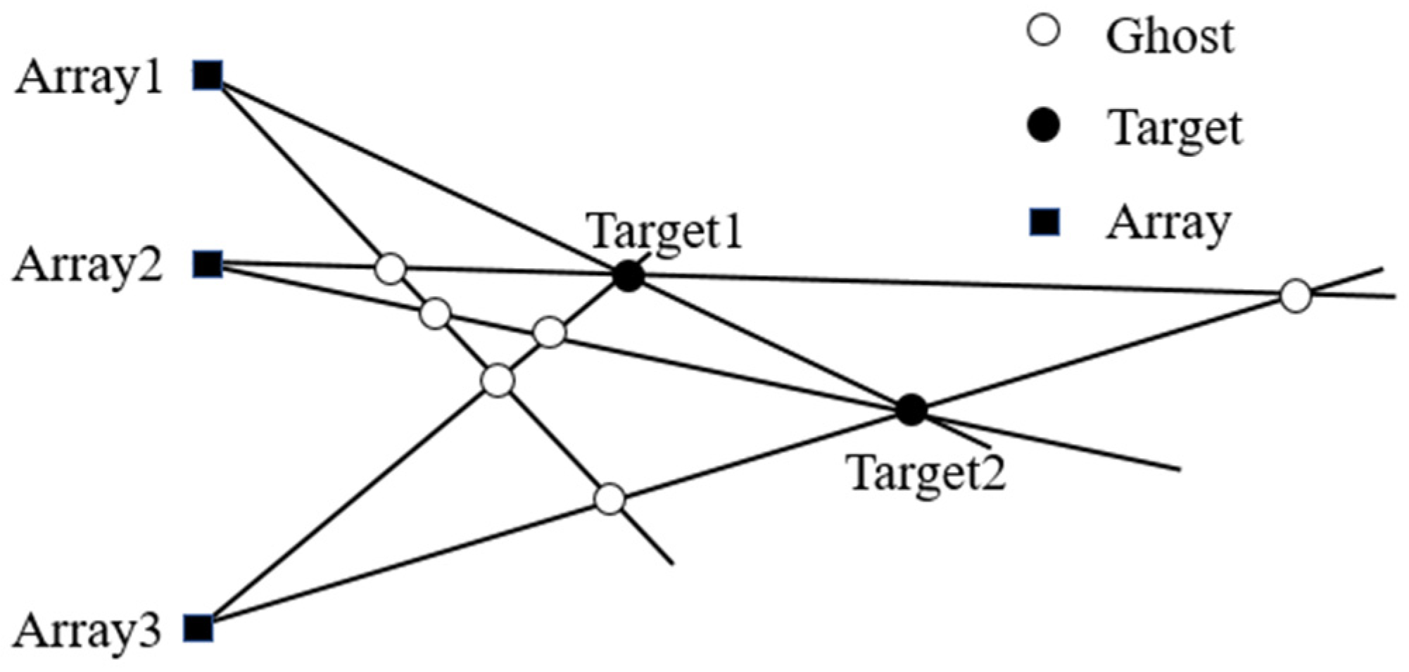
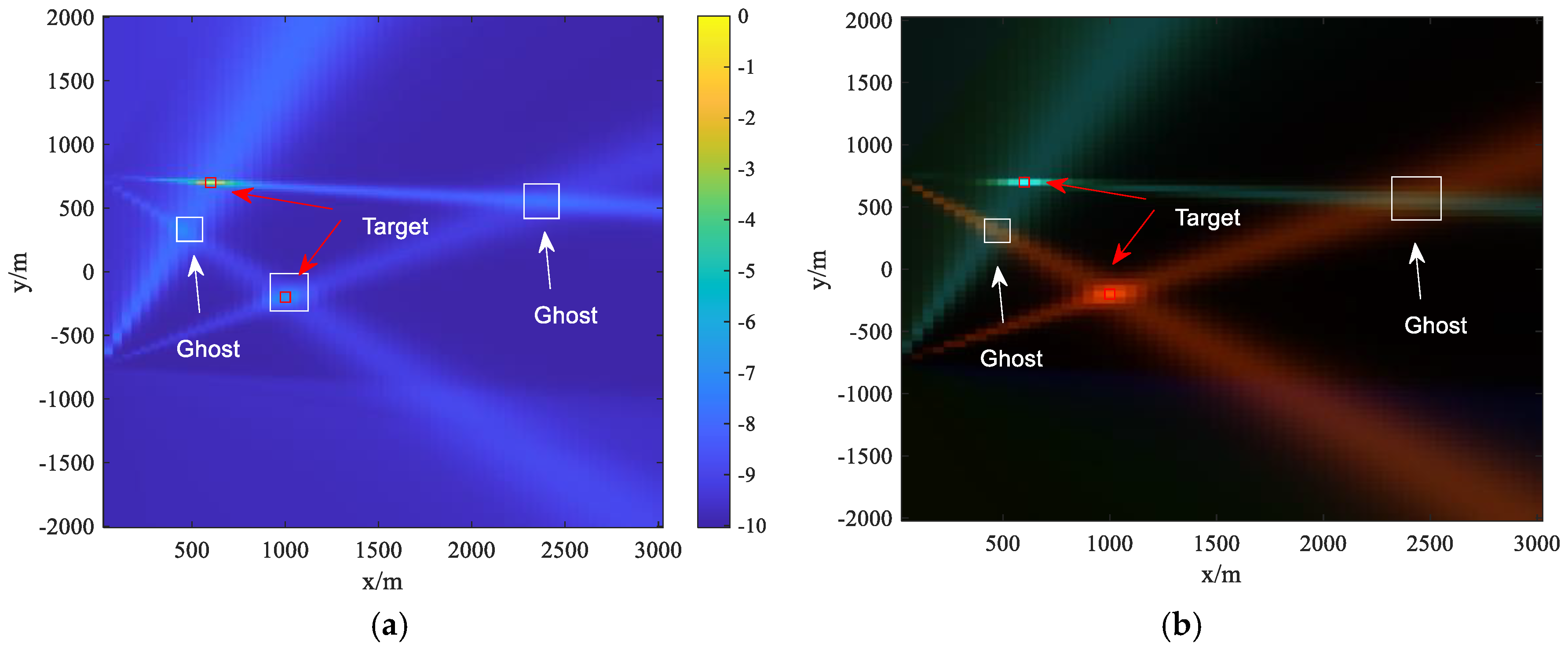
3.1. Generation of Ghosts

In distributed array systems, each array receives signals from specific directions. The geometric configuration shows that the intersection points between lines from different arrays aimed at different targets do not necessarily correspond to actual targets; some of these intersections might be false targets, commonly known as ‘ghosts’. This phenomenon is illustrated in Figure 1. The broadband DPD method, as detailed in Section 2, aggregates the narrowband DPD spatial spectrum matrix along the frequency axis, where the energy peak marks the grid point of the target’s position. By summing along the frequency axis, signal characteristics are cumulated, diminishing the effects of random noise and enhancing the accuracy of target positioning. However, Equation (12) solely relies on the signal’s energy information and may not effectively resolve the presence of ghosts.

To describe the ghost problem in detail, we assume that the number of targets is $K$; the number of arrays is $L$; and $N_T$ and $G$ are the number of detected points and ghosts, respectively, meaning that $N_T=K+G$. The number of lines between different arrays and different targets is $N_K$. Since two non-parallel lines on the same plane only have one intersection point, the number of intersection points, $N_P$, can be calculated from the number of lines as follows:

$$N_P={\displaystyle \frac{\left(N_K\right)!}{2!\left(N_K-2\right)!}}={\displaystyle \frac{1}{2}}LK\left(LK-1\right),$$

(13)

where $\left(\mathbf{·}\right)!$ represents the factorial $\left(n\right)!=n\times \left(n-1\right)\times \cdots \times 2\times 1$. Using the derivation in reference [24], the number of detected points, $N_T$, can be calculated as

$$\begin{array}{l}{N}_T=N_P-LK\left(K-1\right)/2-K\left[L\left(L-1\right)/2-1\right]\\ \hspace{1em} =LK\left(K-1\right)\left(L-1\right)/2+K\end{array}.$$

(14)

with Equation (14), the number of ghosts, $G$, can easily be derived.

This analysis shows that as the number of targets increases, the number of estimated ghosts becomes much greater than the number of real targets. The presence of ghosts substantially compromises the accuracy of passive target detection, particularly in environments where there are marked differences in target strength or when targets are near each other.

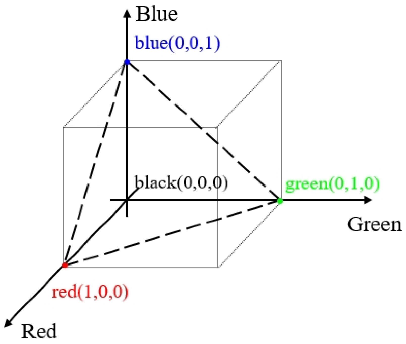
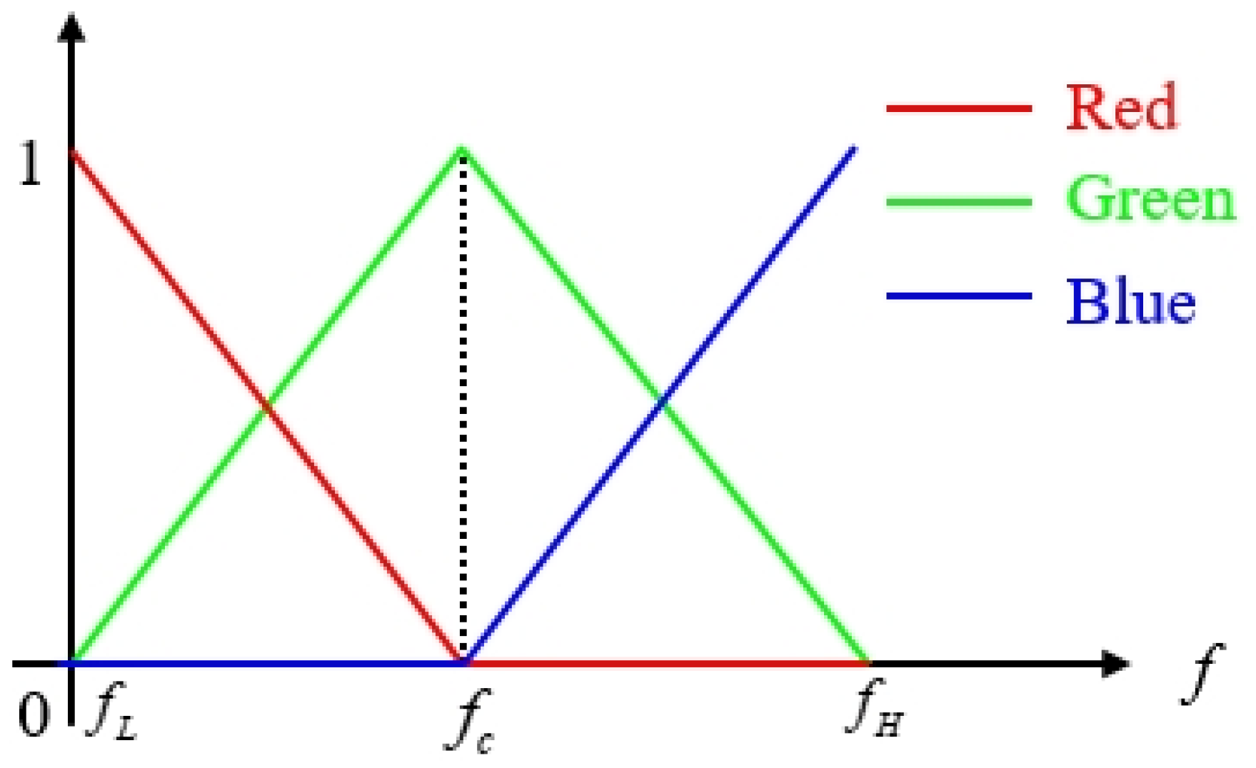
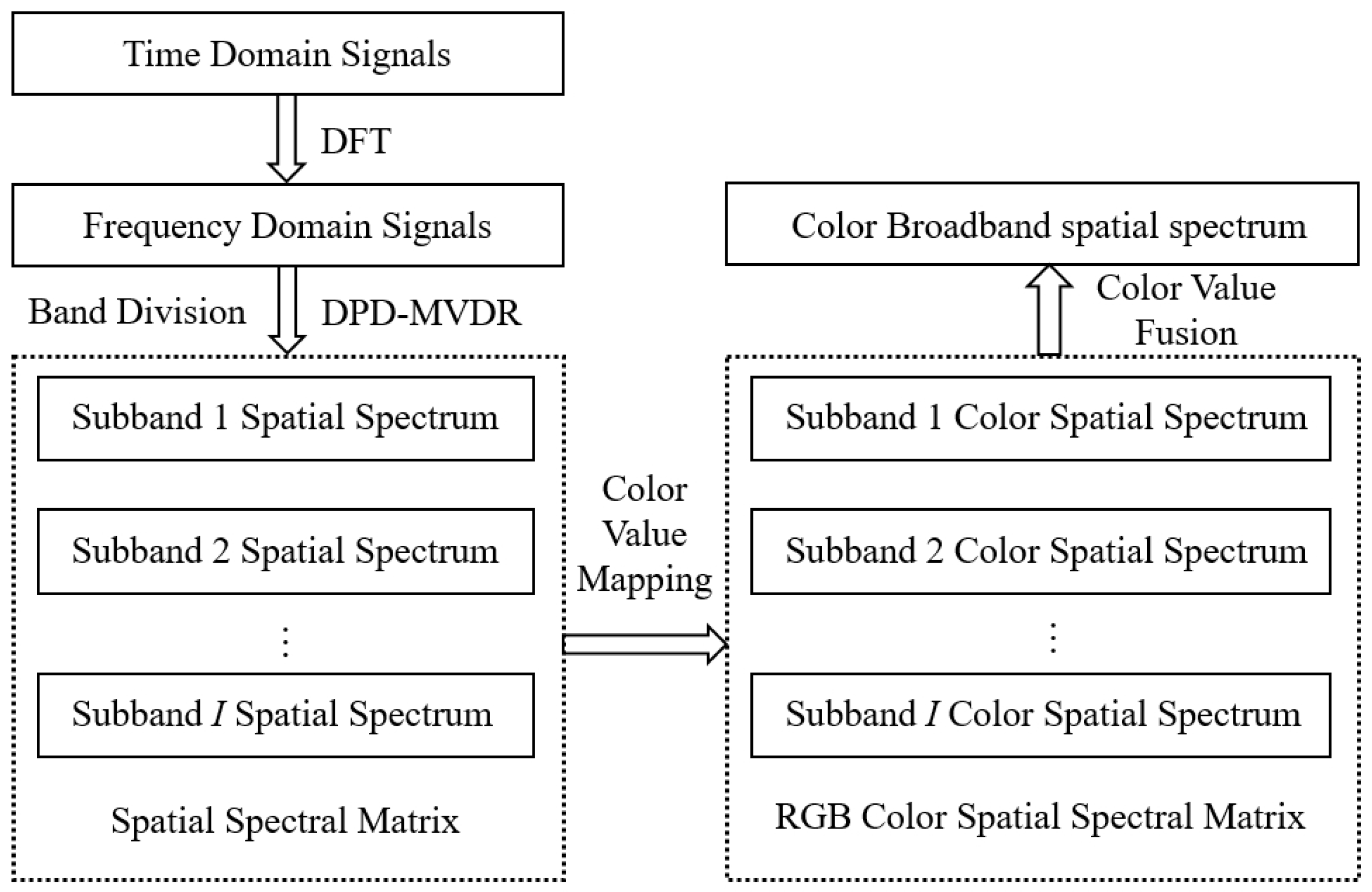
3.2. Distinguishing Ghosts Based on Frequency Coloring

Considering that the signals received by the arrays originate from different sources, they may exhibit certain differences in spectral structure. Leveraging these differences, signal frequency characteristics can discriminate between signals and facilitate data association. In this section, we propose a ghost discrimination method for broadband DPD based on frequency coloring technology. This method employs the three primary colors (red, green, and blue—RGB) to assign distinct color values to the frequency of the sub-bands, mapping each frequency bin to a corresponding color. By visually representing the frequency differences between multiple targets with color, signals with unique frequency structures will appear as distinct colors. The DPD spatial spectrum obtained in this manner utilizes not only the energy information of the signal but also its frequency information, effectively aiding in distinguishing between different targets and identifying ghost signals.

In an RGB image, each pixel corresponds to a combination of three components: red (R), green (G), and blue (B). This type of image can be viewed as a stack of three primary color images [35]. The value range for each RGB component lies between 0 and 255, with red represented by (255, 0, 0), green by (0, 255, 0), and blue by (0, 0, 255) [36]. To simplify the description, we depict the RGB color space as a unit cube, where the RGB component values are normalized to a range of [0, 1], as illustrated in Figure 2.

By recording the spatial spectrum of each sub-band in Equation (11), the DPD spatial spectrum of the wideband signal can be regarded as an $N_f\times \left(X\times Y\right)$-dimensional matrix, where $N_f$ represents the number of sub-bands divided within the bandwidth of interest. $X$ represents the number of grid points along the x-axis, and $Y$ represents the number of grid points along the y-axis. To ensure one-to-one correspondence between the matrix elements, the RGB image is defined as a color pixel group composed of three primary color (R, G, B) matrices with the following dimensions: $N_f\times \left(X\times Y\right)$. Each color pixel is a combination of three color components (R, G, B) at a specific spatial location in the color image.

To map from frequency to color values, a color-value mapping matrix, $\mathit{C}\in {ℝ}^{N_f\times 3}$, needs to be constructed. This matrix assigns each frequency bin to a color. Through this mapping relationship, the energy information and frequency information of the signal are simultaneously utilized. The color-value mapping matrix, $\mathit{C}\in {ℝ}^{N_f\times 3}$, can be expressed as $C={[{\mathit{c}}_1,...,{\mathit{c}}_n,...{\mathit{c}}_{N_f}]}^{\mathrm{T}}\in {ℝ}^{N_f\times 3}$, where $c_n={[r\left(f_n\right),g\left(f_n\right),b\left(f_n\right)]}^{\mathrm{T}}\in {ℝ}^{3\times 1}$ is the RGB component of the mapping matrix, $\mathit{C}$, in the $n$-th sub-band. That is, each sub-band is mapped to one RGB component, $c_n$, representing one color. When designing the coloring strategy, it is important to note that we need to construct the mapping matrix, $\mathit{C}$, according to $c_n$, which incorporates three monotonic functions. This is because color-value mapping non-monotone relations will cause different frequencies that map the same or similar colors.

To ensure consistent discrimination in the frequency mapping, we opt to adjust colors along the diagonal of the RGB color space cube, as depicted in Figure 2. This adjustment follows the dashed lines within two planes of the color space, ensuring a linear relationship between frequency changes and color variations. It can be expressed by the following formula:

$$\begin{array}{l}r(f_n)=\left\{\begin{array}{l}{\displaystyle \frac{1}{f_c-f_L}}\left(f_c-f_n\right),f_n\le f_c\\ \hspace{1em}\hspace{1em} 0\hspace{1em}\hspace{1em}\hspace{1em},f_n>f_c\end{array}\right.\\ g(f_n)=\left\{\begin{array}{c}{\displaystyle \frac{1}{f_c-f_L}}\left(f_n-f_L\right),f_n\le f_c\\ {\displaystyle \frac{1}{f_H-f_c}}\left(f_H-f_n\right),f_n>f_c\end{array}\right.\\ b(f_n)=\left\{\begin{array}{c}\hspace{1em}\hspace{1em}\hspace{1em}0\hspace{1em}\hspace{1em}\hspace{1em},f_n\le f_c\\ {\displaystyle \frac{1}{f_H-f_c}}\left(f_n-f_c\right),f_n>f_c\end{array}\right.\end{array},$$

(15)

where $r\left(f_n\right)$, $g\left(f_n\right)$, and $b\left(f_n\right)$ represent the color value components of red, green, and blue, respectively; $f_n$ is the frequency of the $n$-th sub-band; and $f_H$, $f_c$, and $f_L$ represent the highest frequency, center frequency, and lowest frequency of the signal, respectively. For simplicity, we use $c_n={[r_n,g_n,b_n]}^{\mathrm{T}}$ instead of $c_n={[r\left(f_n\right),g\left(f_n\right),b\left(f_n\right)]}^{\mathrm{T}}$ in the following text.

The RGB color value variation strategy related to frequency is illustrated in Figure 3. In Figure 3, the three colors can be interchanged without affecting the overall functionality. Changing the colors associated with different frequency bins does not alter their effectiveness in distinguishing between actual targets and ghosts.

Let the RGB value corresponding to the $n$-th sub-band be $\left(r_n,g_n,b_n\right)$. The spatial spectrum output of the $n$-th sub-band in the DPD-MVDR method is mapped to the RGB space, which can be expressed by the following formula:

$$\left\{\begin{array}{c}{{\mathit{P}}_n}^{\left(r\right)}=r_n{\mathit{P}}_n\\ {{\mathit{P}}_n}^{\left(g\right)}=g_n{\mathit{P}}_n\\ {{\mathit{P}}_n}^{\left(b\right)}=b_n{\mathit{P}}_n\end{array}\right.,$$

(16)

where ${\mathit{P}}_n$ is the spatial spectrum output of the DPD-MVDR method for the $n$-th sub-band, an $X\times Y$ matrix. The mapping process depicted in Figure 4 shows that the z-axis represents frequency variation, while the x-axis and y-axis represent spatial position variations across the two-dimensional plane. Utilizing this frequency coloring strategy, lower-frequency targets tend to display as red, medium-frequency targets as green, and higher-frequency targets as blue. Additionally, the energy level influences the mapping results; targets with stronger energy appear brighter, whereas those with weaker energy appear darker. When two targets’ energies are concentrated in different frequency bands, the colors corresponding to their positions in the colored broadband spatial spectrum will differ, making it easier to distinguish between them. Conversely, ‘ghosts’ resulting from incorrect data association will display a blend of various colors, markedly different from the colors of real targets. A grid point where there is no signal will appear black due to the low energy on the grid point.

In the RGB color model, red, green, and blue are recognized as the three primary colors of light; when two or more lights are mixed, the resulting color is a composite of the color values of each contributing light source [37]. Consequently, the sub-band output spatial spectrum, once mapped to the RGB space per Equation (16), can be aggregated, culminating in the broadband spatial spectrum output of the DPD-MVDR method in the RGB space, detailed below.

$$\left\{\begin{array}{c}{\mathit{P}}^{\left(r\right)}={\displaystyle \sum _{n=1}^N{r}_n{\mathit{P}}_n}\\ {\mathit{P}}^{\left(g\right)}={\displaystyle \sum _{n=1}^N{g}_n{\mathit{P}}_n}\\ {\mathit{P}}^{\left(b\right)}={\displaystyle \sum _{n=1}^N{b}_n{\mathit{P}}_n}\end{array}\right..$$

(17)

The specific implementation process of the proposed method is illustrated in Figure 5. The broadband spectrum is divided into multiple sub-bands, and target positions are solved in the frequency domain. The peak values of the spatial spectrum for each sub-band are extracted to obtain the target position. Then, using the frequency coloring strategy, each sub-band’s spatial spectrum is mapped to color values. Finally, summing along the frequency dimension, different colors represent different frequencies, while both the energy and frequency information about the signal is utilized.

The specific steps of the proposed ghost-distinguishing method are shown in Algorithm 1.

Algorithm 1: Ghost discrimination method for broadband DPD based on frequency coloring

1:  Input: The number of arrays, $L$; the speed of sound in water, $c$; array positions, ${\mathbf{P}}_l$; received signals, $x_l(t)$; number of elements, $M_l$; and $l=1,\cdots ,L$. 2:   Initialize: the number of sub-bands, $I$; the number of data segments, $Q$; the target bandwidth, $\left[f_L,f_H\right]$. 3:   for $i=1,\cdots ,I$ do: 4:    for $l=1,\cdots ,L$ do: 5:      Compute ${\overline{x}}_l(f_i,q)$ by Equation (4). 6:      Compute ${\widehat{R}}_{l,i}$ by Equation (5). 7:      Compute ${\widehat{\mathit{p}}}_{i-\mathrm{MVDR}}$ by Equation (11). 8:    end 9:    Obtain $\left(r_i,g_i,b_i\right)$ by Equation (15). 10:     Compute ${{\mathit{P}}_i}^{\left(r,g,b\right)}$ by Equation (16). 11:  end 12:  Compute ${\mathit{P}}^{\left(r,g,b\right)}$ by Equation (17). 13:  Output: ${\mathit{P}}^{\left(r,g,b\right)}$.

4. Simulation and Experiment

In this section, the effectiveness of the proposed method in distinguishing between actual targets and ghosts is analyzed and compared with the MVDR-DPD method. Additionally, we process data from the SwellEx-96 shallow-water experiment to validate the applicability and performance of the proposed method.

4.1. Numerical Examples

The simulation system comprises $L=2$ uniform linear arrays with the same array structure. The array comprises $M_l=21,l=1,2$ omnidirectional sensors with an intersensor spacing of 3 m. The configuration of the distributed array system consists of two linear arrays with the first sensors located at [0, 780] m, and [0, −720] m. The positions of these arrays are depicted in Figure 6. For the grid search, an area spanning [0, 3000] m on the x-axis and [−2000, 2000] m on the y-axis is considered, divided into a grid interval of 50 m. The speed of sound in the water is set at 1500 m/s. The simulated signal sampling frequency is $f_s=2.5 \mathrm{k}\mathrm{H}\mathrm{z}$, and the frequency of the signal is set at $f=\left[f_L,f_H\right]$. The time interval, $T$, of the signals is 4 s. The observed time interval, [0, T], can be partitioned into 39 sections with 50% overlap and the length of each section is 500 samples (i.e., 0.16 s). The number of FFT points, $N$, is 500, equal to the length of each section. The noise added in the simulation is wide-sense stationary zero-mean complex Gaussian white noise.

In scenarios involving multiple targets, the RGB coloring strategy assigns distinct color values to each sub-band frequency, enhancing the visual differentiation of targets within the specified grid. The frequency band of our data processing should cover the frequency band range of all signals. Thus, $f_L=\min \left(f_{L1},\cdots ,f_{LK}\right)$ and $f_H=\max (f_{H1},\cdots ,f_{HK})$, where $K$ is the number of the signal. The SNR of the $k$-th signal at the $l$-th array is defined as the ratio of the signal power to the noise power in the processing bandwidth, denoted as $\mathrm{S}\mathrm{N}{\mathrm{R}}_{l,k}=10\lg \left({\displaystyle {\sum }_{f_n=f_L}^{f_H}{\sigma }_{k,f_n}}/{\displaystyle {\sum }_{f_n=f_L}^{f_H}{\eta }_{l,f_n}}\right)$. In the simulation, we consider the cylindrical propagation assumption under shallow sea conditions to approximate the signal propagation loss, ${\alpha }_{l,k}$, and reflect it in the SNR of different signals. The SNR at the second array is scaled according to the SNR at the first array, expressed as follows:

$$\mathrm{S}\mathrm{N}{\mathrm{R}}_{2,k}=\mathrm{S}\mathrm{N}{\mathrm{R}}_{1,k}-10\lg \left(D_{2,k}/D_{1,k}\right),$$

(18)

where $D_{1,k}$ is the distance from the $k$-th signal to the first array, and $D_{2,k}$ is the distance from the $k$-th signal to the second array.

In this section, we present numerical results to demonstrate the properties of the proposed method and to compare it with the DPD−MVDR method [17]. Given that variations in target power and the number of targets can cause ghosts to obscure real targets and impact positioning accuracy, we have conducted simulations under the three following conditions.

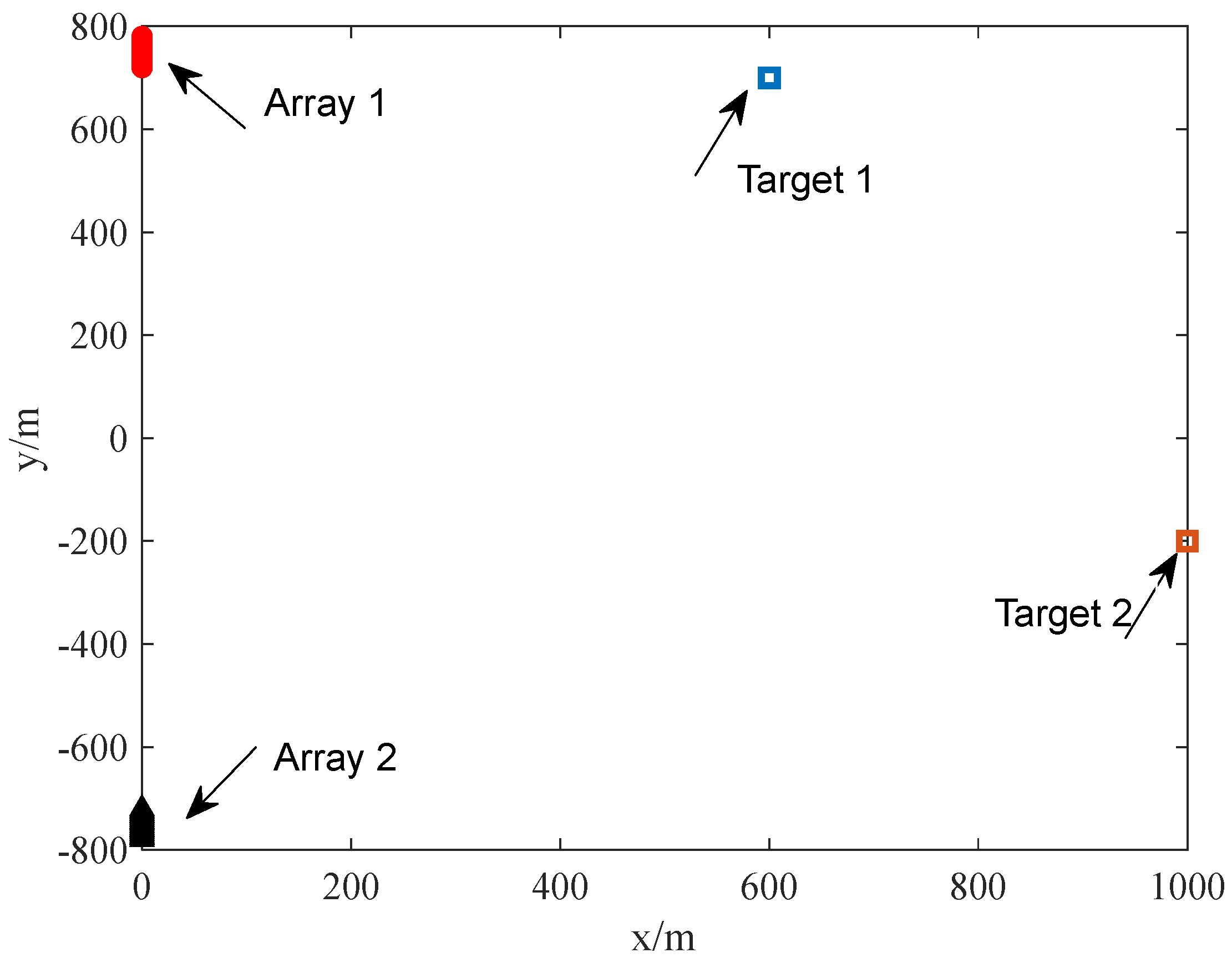
• Dual-Target Localization with Equal Intensity

Consider two signals incident from the far field to two arrays. The positional relationship between the targets and arrays is illustrated in Figure 6. The location of target 1 is [600, 700] m, with a frequency range of [250, 500] Hz. The received signal power at array 1 is denoted as $P_1$, where $P_1=10\lg \left({\displaystyle {\sum }_{f_n=f_L}^{f_H}{\sigma }_{1,f_n}}\right)$ is −10 dB. The location of target 2 is [1000, −200] m, with a frequency range of [125, 250] Hz. The received signal power at array 1 is denoted as $P_2$, where $P_2=10\lg \left({\displaystyle {\sum }_{f_n=f_L}^{f_H}{\sigma }_{2,f_n}}\right)$ is also −10 dB. Assuming a uniform noise field, the noise power at each array is represented by $P_n$, where $P_n=10\lg \left({\displaystyle {\sum }_{f_n=f_L}^{f_H}{\eta }_{f_n}}\right)$ is 0 dB.

The spatial spectra of the two methods are displayed in Figure 7. The two arrays estimate four intersection points, of which only two are actual signals, and the other two are ghosts. In the spatial spectrum of the DPD-MVDR method shown in Figure 7a, the two intersection points within the red box that exhibit stronger energy are identified as signals. Conversely, the two intersection points in the white box displaying weaker energy are categorized as ghosts. However, since the number of targets is not predetermined in real situations, relying solely on energy strength to identify targets can lead to misidentifying ghosts as actual targets.

According to the coloring strategy illustrated in Figure 3, the signal color will change from red to green and then to blue as the frequency increases, where $f_L$ corresponds to 125 Hz and $f_H$ corresponds to 500 Hz. The frequency band division and mapping are performed by Equation (15). We assume that each target maintains a consistent frequency structure; thus, intersections of rays of the same color indicate a target, while intersections involving rays of different colors are identified as ghosts, resulting from the convergence of false peaks from different targets. In Figure 7b, using the RGB color spatial spectrum of the proposed method, the intersection of two blue-green rays corresponds to target 1, and the intersection of two orange-red rays to target 2. The simulation results demonstrate that the proposed method can effectively utilize frequency information to distinguish between real targets and ghosts, achieving accurate localization.

B.

Dual-Target Localization with Unequal Intensity

Under the same positional and frequency conditions for arrays and targets outlined in Simulation A, target 1 emits a signal with a power of −5 dB, while target 2 emits a weaker signal with a power of −10 dB. As depicted in Figure 8a, with the varying target strengths, one intersection point clearly shows stronger energy, whereas the three intersections marked in the white box display weaker energy, making it challenging to ascertain whether they represent real targets or ghosts. Figure 8b demonstrates how the proposed method leverages frequency information to effectively differentiate between ghosts and real targets based on the color of the intersection lines. With frequency coloring applied, the actual targets are clearly marked by two intersection points indicated by the red arrows.

C.

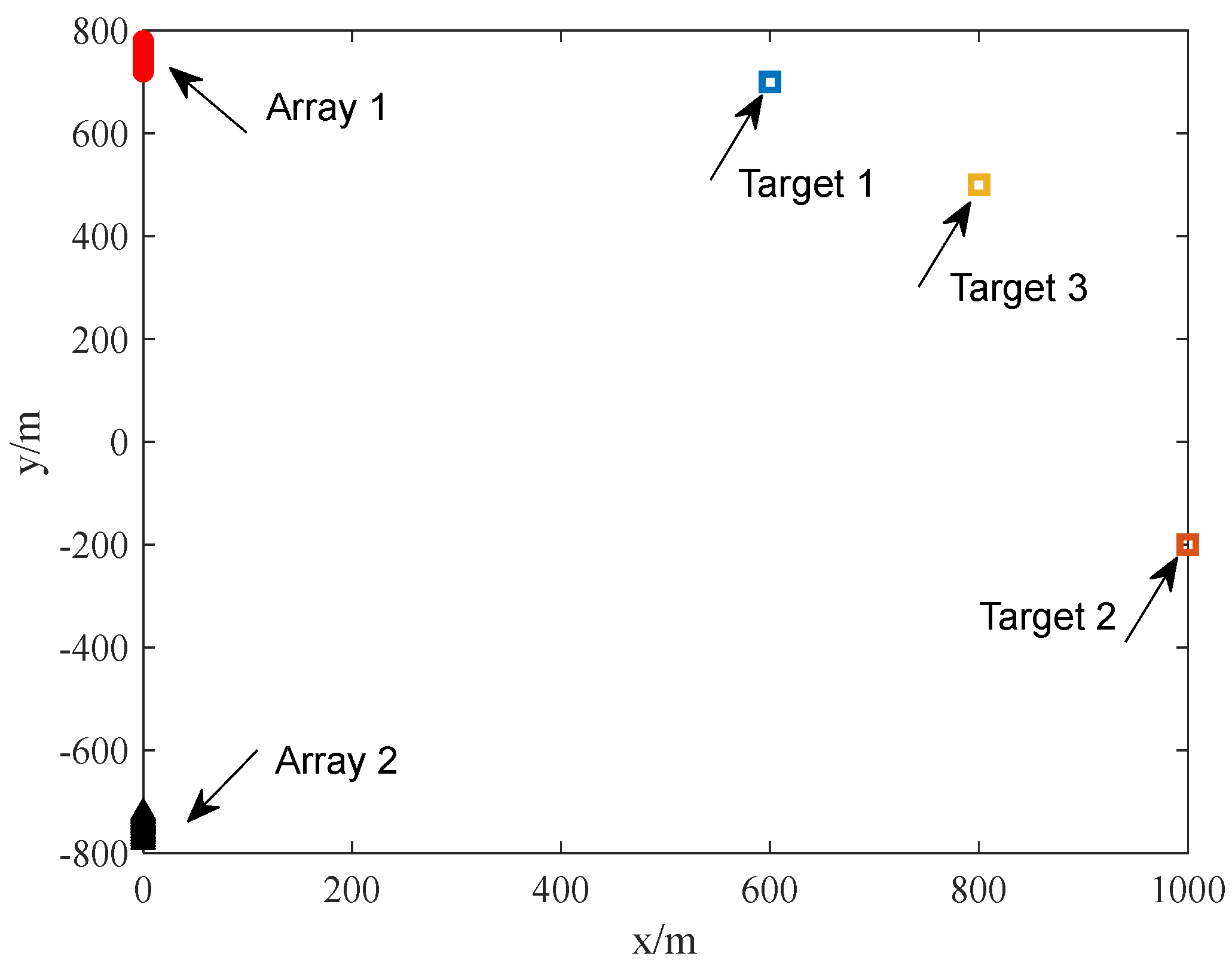
Multi-Target Localization

Under the same condition outlined in Simulation A, an additional target with a signal power of −10 dB is introduced. This new target is positioned near target 1 at coordinates [800, 500] m, with the frequency band of its incident signals ranging from 250 Hz to 750 Hz. This range overlaps with the frequency band of target 1. The spatial configuration of the targets and arrays is depicted in Figure 9.

In the case of multiple targets, there will be more points with strong energy in the spatial spectrum, which are easily mistaken for targets. Figure 10 displays the estimated spatial spectrum of the DPD-MVDR method alongside the proposed method for three targets. Figure 10a shows that the spatial spectrum of DPD-MVDR has nine prominent energy intersections. We have highlighted five intersections with strong energy in the figure, but it is challenging to directly discern which of these intersections are actual targets solely based on the DPD-MVDR spatial spectrum. The RGB color spatial spectrum of the proposed method is shown in Figure 10b, using the frequency information of the signal to differentiate between targets. According to the design strategy of the mapping matrix, a target corresponds to an intersection point generated by the same color ray, while intersections formed by rays of differing colors are considered ghosts. Within this framework, targets 1, 2, and 3 are represented by green, red, and blue, respectively. This can directly identify which of the five intersections with strong energy belongs to the real target.

D.

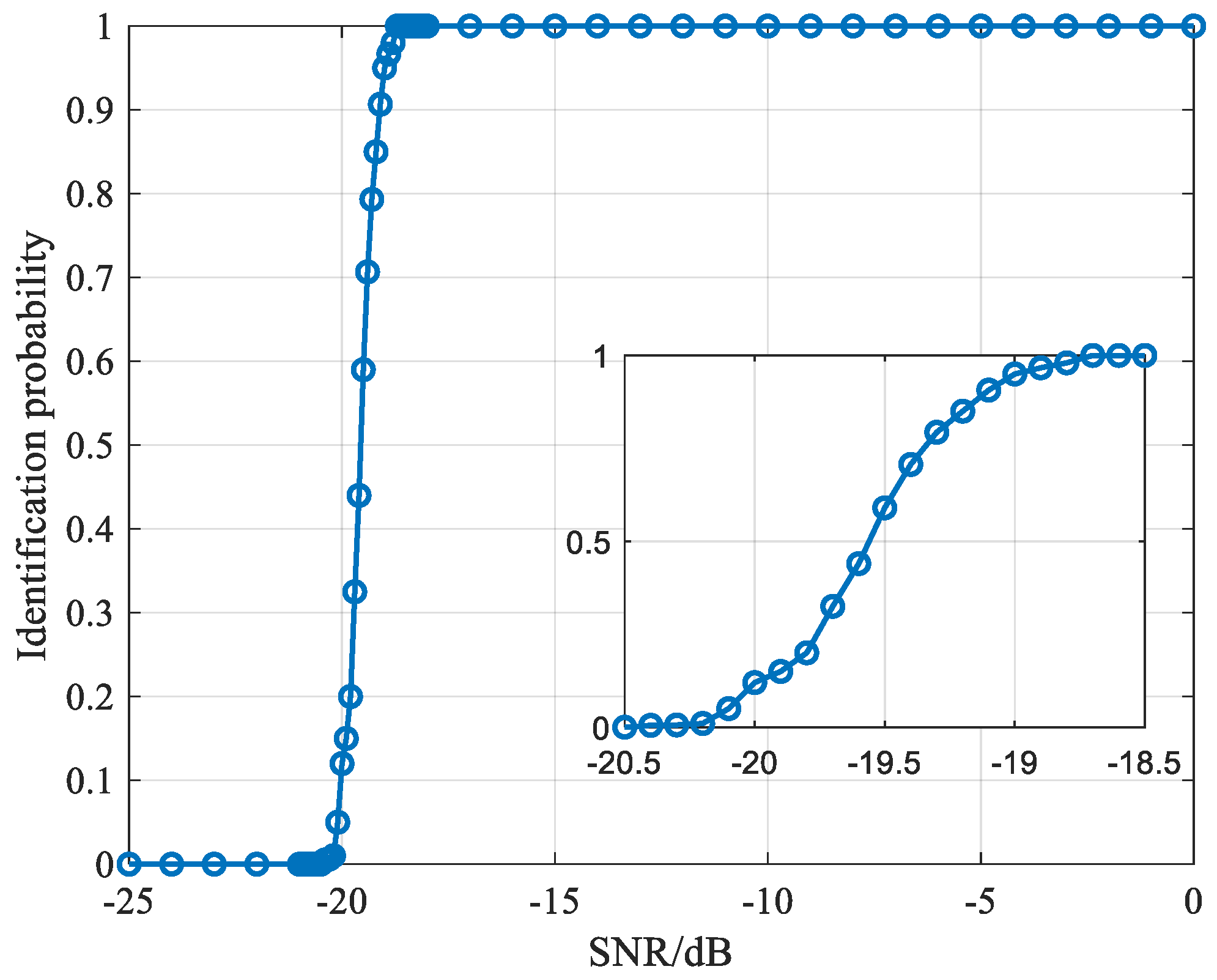
Ghost-Distinguishing Ability

In practical applications, different environmental noise levels will affect the ghost discrimination performance of the proposed method. Thus, its statistics on the probability of correctly distinguishing targets from ghosts are analyzed in this subsection. Based on the proposed coloring strategy, the lines in the RGB color spatial spectrum that connect one target and different subarrays will have the same color. This is because the frequency structure of one target is almost the same despite being received by different subarrays. Therefore, in all targets and ghosts, the closer the color of two different lines in the RGB color spatial spectrum is, the more likely their intersection is a target. RGBs and HSVs are both among the most important color image types, derived from the RGB and HSV color spaces, respectively [38,39]. Similarly to RGB images, HSV images consist of three channels: hue (H), saturation (S), and value (V). Among them, color information is primarily represented by the H channel, while S reflects the purity of the color, and V represents brightness [40]. Given that the frequency mapping in this study primarily relies on distinctions in hue, the HSV color space is selected to measure color similarity in this subsection. After converting the RGB color space into a normalized HSV color space, the distance between two pixels in the color spatial spectrum can be calculated as follows:

$$d_{\mathrm{HSV}}={\displaystyle \frac{\left|h_i-h_j\right|+\left|s_i-s_j\right|+\left|v_i-v_j\right|}{3}}$$

(19)

where $h_i$, $s_i$, and $v_i$ represent the hue, saturation, and value of the $i$-th pixel, respectively. When $i=j$, it indicates that the two pixels overlap. The closer the HSV values of two pixels are, the smaller their distance approaches 0. Conversely, the greater the differences between two pixels, the closer their distance approaches 1.

Using the distance between two pixels in the HSV color space, we evaluated the model’s performance in correctly distinguishing between targets and ghosts under the same conditions as Simulation C, as the SNR changes. To mark the color of a line connecting a target to a subarray in the RGB color spatial spectrum, we selected 10 consecutive pixels along the line with uniform colors and no surrounding interference pixels. The average RGB value of these pixels was computed and converted into normalized HSV values to calculate the color distance between them. The intersections of three groups of lines with the smallest color distances were identified as the estimated target locations. If the estimated targets correspond to the correct intersection of the target–subarray line, the targets and ghosts are considered successfully distinguished. In this simulation, 300 Monte Carlo experiments were conducted to calculate the probability of correct discrimination. Figure 11 shows that the proposed method can accurately distinguish between targets and ghosts at an SNR above −18 dB.

4.2. Application to the SWellEx-96 Data

In this section, the performance of the proposed method is verified based on the SWellEx-96 experiment. The SWellEx-96 experiment was conducted from 10 to 18 May 1996, approximately 12 km off the coast near Point Loma, San Diego, California [41]. The data set comes from the SWellEx-96 shallow-water evaluation cell experiment, Event S59, which features two horizontal line arrays: HLA North and HLA South. These arrays were deployed on the seabed about 3 km apart at water depths of 213 m for HLA North and 198 m for HLA South. Each array consists of 32 elements, and both arrays have a slight bow. During processing, data from the first 27 sensors of both arrays are processed.

During Event S59, sources were simultaneously towed along by the R/V Sproul as an isobath, and the acoustic sources transmitted various broadband and multitone signals at frequencies between 49 Hz and 400 Hz. Additionally, Event S59 included a ship as a loud interferer. Both arrays (HLA North, and HLA South) recorded the entire 65 min duration of the event, which began at 11:45 GMT and ended at 12:50 GMT. The R/V Sproul initiated its course between and slightly east of the two HLAs, traveling northward along the 180 m isobath at a speed of 5 knots (approximately 2.5 m/s). The path of the interferer of interest began west of all arrays, proceeded southeast and between the two HLAs, and concluded east of the arrays (Figure 12a).

To better illustrate the position of the two targets, we selected a 10 s data segment starting at the 30 min mark of the record. At this moment, the distance between the two cooperative targets and the two arrays is relatively close. The geolocation of the interferer provided on the data website is 32°38′35.341″ N and 117°22′24.904″ W. We converted these coordinates into 2-D Cartesian coordinates (−1571, 1725) m. The target’s position was mapped relative to the interferer, resulting in coordinates of (1061, 5856) m (Figure 12b).

The surface ship acted as an interference in SWellEx-96 Event S59, and the spectrum information of the radiated noise signal is unknown. Figure 13 shows a time–frequency diagram of the intercepted data received by the two arrays. The surface ship and the signal can be detected across a wide range of frequencies, particularly from 20 Hz to 400 Hz. Therefore, we selected the frequency band containing the processing frequency band of two cooperative targets to demonstrate the capabilities of our proposed method. The data were sampled at 3276.8 Hz, and we selected 76 frequency bins with 5 Hz increments.

Figure 14a,b present the spatial spectra for the DPD-MVDR method and the proposed method, respectively. The mapping between the sub-bands and RGB is shown in Figure 3. There is an interference and a signal at the red pentagram and the red box, respectively. In Figure 14a, due to the influence of 37sidelobes and unknown interference, multiple bright lines appear in the spatial spectrum of the DPD-MVDR method. Among these, the two bright spots indicated by white arrows are ghosts, which can be easily misinterpreted as signals. By contrast, Figure 14b uses the differences in the frequency structure between signals, yielding an effective distinction between ghosts and real targets compared with the results in the spatial spectrum of the DPD-MVDR method. Figure 14b shows that the positions indicated by the white arrows correspond to the intersections of yellow and blue lines, suggesting that they are not actual signals of interest. Furthermore, in the chosen data segment, since the interference is located near the endfire of both arrays, there is a prominent bright region near the location of the interference. Next, we will analyze the unknown interference shown in Figure 14 through bearing-time records (BTRs) and explain the color mapping of the target through the known frequency structure.

Using the BTR of the signals received by the two arrays, we can further analyze the unknown interference presented in Figure 14. When describing the target’s bearing, we define 0° as due north, with positive increments in a clockwise direction. Figure 14 shows that the target estimated by HLA North includes a bright line with strong energy at an angle of approximately 315°. Through the BTR of the signals received by HLA North in Figure 15a, we can see that at around the 30 min mark—apart from the target and interference under test—HLA North identifies a strong, unknown interference at a constant angle of around 315°, corresponding to the bright line in the upper-left corner of the localization results in Figure 14. Figure 15b shows that HLA South does not detect this strong interference. Therefore, there is only one ray in Figure 14, which does not locate this unknown strong interference.

Notably, there are subtle differences in the colors of the two arrays in the position estimation of the signal. This is because, in real environments, signal energy attenuates with propagation distance, and the difference in distances between the target and the two arrays will lead to differences in the spectral energy of the received signals. The time–frequency diagrams for the two arrays—shown during the time of interest in Figure 13—reveal subtle differences in the spectrum frequency structure of the signals contained in HLA North and HLA South. Therefore, after frequency coloring, the signals estimated by HLA North should appear bluish-green, whereas those estimated by HLA South should be bluer. This is consistent with the actual estimated results shown in Figure 14b, but this does not affect the correctness of our judgment. The experimental data demonstrate that considering the spectral differences in the signals in the spatial spectrum effectively distinguishes the targets from ghosts, thereby improving the accuracy of the DPD-MVDR method.

5. Conclusions

This study proposes a DPD algorithm based on frequency coloring, where the frequency of broadband signals is represented through color, increasing the efficiency of signal information utilization and effectively distinguishing real targets from ghosts in multi-target scenarios. Traditional DPD algorithms for broadband target localization typically combine spatial spectra across sub-bands and distinguish signals based on energy differences. However, in multi-target scenarios, positioning accuracy is affected not only by interference but also by ghosts. To enhance the ability of the DPD algorithm to distinguish real targets and ghosts, this study leverages the spectral differences between multiple targets to color the spatial spectrum of each sub-band so that targets with different spectral structures correspond to different colors. This distinguishes between different targets and ghosts. Numerical simulations demonstrate that the proposed method effectively distinguishes targets and ghosts even at a low SNR level. The results of the SWellEx-96 data set processing confirmed the effectiveness of the proposed method in distinguishing between targets and ghosts.

Complex multi-target scenarios are a great challenge for most localization methods. However, the proposed method offers an intuitive and effective solution for multi-target scenarios. Compared with original DPD methods, the proposed approach provides greater potential for addressing the complex scenarios. The potential application of this method to larger arrays and more intricate target environments is being explored, requiring further investigation into more generalized localization methods.

References

1. Tzafri, L.; Weiss, A.J. High resolution direct position determination using MVDR. IEEE Trans. Wirel. Commun. 2016, 15, 6449–6461. [Google Scholar] [CrossRef]
2. Doanay, K. Bearings-only target localization using total least squares. Signal Process. 2005, 85, 1695–1710. [Google Scholar]
3. Wang, Z.; Luo, J.A.; Zhang, X.P. A Novel Location-Penalized Maximum Likelihood Estimator for Bearing-Only Target Localization. IEEE Trans. Signal Process. 2012, 60, 6166–6181. [Google Scholar] [CrossRef]
4. Stansfield, R.G. Statistical Theory of DF Fixing. J. IEE 1947, 94, 762–770. [Google Scholar]
5. Gavish, M.; Weiss, A.J. Perfromance analysis of bearing-only target location algorithms. IEEE Trans. Aerosp. Electron. Syst. 1992, 28, 817–828. [Google Scholar] [CrossRef]
6. Pattipati, K.R.; Deb, S.; Bar-Shalom, Y.; Washburn, R. A new relaxation algorithm and passive sensor data association. IEEE Trans. Autom. Control 1992, 37, 198–213. [Google Scholar] [CrossRef]
7. Bishop, A.N.; Pathirana, P.N. Localization of emitters via the intersection of bearing lines: A ghost elimination approach. IEEE Trans. Veh. Technol. 2007, 56, 3106–3110. [Google Scholar] [CrossRef]
8. Gholami, M.R.; Gezici, S.; Strom, E.G. A Concave-Convex Procedure for TDOA Based Positioning. IEEE Commun. Lett. 2013, 17, 765–768. [Google Scholar] [CrossRef]
9. Smith, J.; Abel, J. Closed-form least-squares source location estimation from range-difference measurements. IEEE Trans. Acoust. Speech Signal Process. 1987, 35, 1661–1669. [Google Scholar] [CrossRef]
10. Chan, Y.T.; Ho, K.C. A simple and efficient estimator for hyperbolic location. IEEE Trans. Signal Process. 1994, 42, 1905–1915. [Google Scholar] [CrossRef]
11. Wang, Y.; Wu, Y. An Efficient Semidefinite Relaxation Algorithm for Moving Source Localization Using TDOA and FDOA Measurements. IEEE Commun. Lett. 2017, 21, 80–83. [Google Scholar] [CrossRef]
12. Wang, G.; Li, Y.; Ansari, N. A Semidefinite Relaxation Method for Source Localization Using TDOA and FDOA Measurements. IEEE Trans. Veh. Technol. 2013, 62, 853–862. [Google Scholar] [CrossRef]
13. So, H.C. Source Localization: Algorithms and Analysis. In Handbook of Position Location: Theory, Practice, and Advances, 2nd ed.; Zekavat, R., Buehrer, R.M., Eds.; Wiley-IEEE Press: Hoboken, NJ, USA, 2011; pp. 25–66. [Google Scholar]
14. Weiss, A.J. Direct position determination of narrowband radio frequency transmitters. IEEE Signal Process. Lett. 2004, 11, 513–516. [Google Scholar] [CrossRef]
15. Wax, M.; Kailath, T. Decentralized processing in sensor arrays. IEEE Trans. Acoust. Speech Signal Process. 1985, 33, 1123–1128. [Google Scholar] [CrossRef]
16. Weiss, A.J. Direct position determination of narrowband radio transmitters. In Proceedings of the 2004 IEEE International Conference on Acoustics, Speech, and Signal Processing, Montreal, QC, Canada, 17–21 May 2004. [Google Scholar]
17. Amar, A.; Weiss, A.J. Analysis of the direct position determination approach in the presence of model errors. In Proceedings of the 2004 23rd IEEE Convention of Electrical and Electronics Engineers in Israel, Tel-Aviv, Israel, 6–7 September 2004. [Google Scholar]
18. Amar, A.; Weiss, A.J. Direct position determination of multiple radio signals. In Proceedings of the 2004 IEEE International Conference on Acoustics, Speech, and Signal Processing, Montreal, QC, Canada, 17–21 May 2004. [Google Scholar]
19. Oispuu, M.; Nickel, U. 3D passive source localization by a multi-array network: Noncoherent vs. coherent processing. In Proceedings of the International ITG Workshop on Smart Antennas, Bremen, Germany, 23–24 February 2010. [Google Scholar]
20. Picard, J.S.; Weiss, A.J. Direction finding of multiple emitters by spatial sparsity and linear programming. In Proceedings of the 2009 9th International Symposium on Communications and Information Technology, Icheon, Republic of Korea, 28–30 September 2009. [Google Scholar]
21. Picard, J.S.; Weiss, A.J. Localization of Multiple Emitters by Spatial Sparsity Methods in the Presence of Fading Channels. In Proceedings of the 2010 7th Workshop on Positioning, Navigation and Communication, Dresden, Germany, 11–12 March 2010. [Google Scholar]
22. Jean, O.; Weiss, A.J. Passive Localization and Synchronization Using Arbitrary Signals. IEEE Trans. Signal Process. 2014, 62, 2143–2147. [Google Scholar] [CrossRef]
23. Wang, G.; Gao, C.; Razul, S.G.; See, C.M.S. A new direct position determination algorithm using multiple arrays. In Proceedings of the 2018 IEEE 23rd International Conference on Digital Signal Processing (DSP), Shanghai, China, 19–21 November 2018. [Google Scholar]
24. Naus, H.W.L.; van Wijk, C.V. Simultaneous localization of multiple emitters. IEE Proc. Radar Sonar Nav. 2004, 151, 65–70. [Google Scholar] [CrossRef]
25. Reed, J.D.; da Silva, C.R.C.M.; Buehrer, R.M. Multiple-source localization using line-of-bearing measurements: Approaches to the data association problem. In Proceedings of the MILCOM 2008-2008 IEEE Military Communications Conference, San Diego, CA, USA, 16–19 November 2008. [Google Scholar]
26. Kanzawa, Y.; Miyamoto, S. Generalized fuzzy c-means clustering and its property of fuzzy classification function. J. Adv. Comput. Intell. Intell. Inform. 2021, 25, 73–82. [Google Scholar] [CrossRef]
27. Campello, R.J.; Moulavi, D.; Sander, J. Density-based clustering based on hierarchical density estimates. In Advances in Knowledge Discovery and Data Mining, Proceedings of the Pacific-Asia Conference on Knowledge Discovery and Data Mining, Gold Coast, Australia, 14–17 April 2013; Springer: Berlin/Heidelberg, Germany, 2013. [Google Scholar]
28. Deng, Z.; Wang, Z.; Zhang, T.; Zhang, C.; Si, W. A novel density-based clustering method for effective removal of spurious intersections in bearings-only localization. EURASIP J. Adv. Signal Process. 2023, 2023, 19. [Google Scholar] [CrossRef]
29. Makhoul, J.; Roucos, S.; Gish, H. Vector quantization in speech coding. Proc. IEEE 1985, 73, 1551–1588. [Google Scholar] [CrossRef]
30. Schell, S.V.; Calabretta, R.A.; Gardner, W.A.; Agee, B. Cyclic MUSIC algorithms for signal-selective direction estimation. In Proceedings of the International Conference on Acoustics, Speech, and Signal Processing, Glasgow, UK, 23–26 May 1989. [Google Scholar]
31. Iqbal, A.; Gans, N.R. Localization of classified objects in SLAM using nonparametric statistics and clustering. In Proceedings of the 2018 IEEE/RSJ International Conference on Intelligent Robots and Systems (IROS), Madrid, Spain, 1–5 October 2018. [Google Scholar]
32. Strecke, M.; Stuckler, J. Em-fusion: Dynamic object-level SLAM with probabilistic data association. In Proceedings of the 2019 IEEE/CVF International Conference on Computer Vision (ICCV), Seoul, Republic of Korea, 27 October 2019. [Google Scholar]
33. Wang, L.; Yang, Y.; Liu, X. A distributed subband valley fusion (DSVF) method for low frequency broadband target localization. J. Acoust. Soc. Am. 2018, 143, 2269–2278. [Google Scholar] [CrossRef] [PubMed]
34. Brandwood, D.H. A complex gradient operator and its application in adaptive array theory. IEE Proc. Radar Sonar Nav. 1983, 130, 11–16. [Google Scholar]
35. Gonzalez, R.C.; Woods, R.E.; Eddins, S.L. Digital Image Processing Using MATLAB, 2nd ed.; Ruan, Q., Ed.; Tsinghua University Press: Beijing, China, 2013; pp. 205–209. [Google Scholar]
36. Zhang, D.; Fan, W.; Xu, L.; Zhang, X. A method of detecting and displaying passive sonar broadband target based on color processing. Techn. Acoust. 2021, 40, 556–559. [Google Scholar]
37. Wang, C.; Liu, X.; Sun, C. Passive sonar broadband energy detection using frequency coloring. J. Harbin Eng. Univ. 2021, 42, 456–462. [Google Scholar]
38. Ashraf, S. Towards Shrewd Object Visualization Mechanism. Trends Comput. Sci. Inf. Technol. 2020, 5, 097–102. [Google Scholar]
39. Kim, S.; You, J. Efficient LUT Design Methodologies of Transformation between RGB and HSV for HSV Based Image Enhancements. J. Electron. Eng. Technol. 2024, 19, 4551–4563. [Google Scholar] [CrossRef]
40. Flores, V.P.; Gómez, D.; Castro, J.; Montero, J. New Aggregation Approaches with HSV to Color Edge Detection. Int. J. Comput. Int. Syst. 2022, 15, 78. [Google Scholar] [CrossRef]
41. SWellEx-96 Experiment Acoustic Data. UC San Diego Library Digital Collections. 2015. Available online: https://library.ucsd.edu/dc/collection/bb3312136z (accessed on 29 October 2024).
42. The SWellEx-96 Experiment. Marine Physical Lab. 2003. Available online: https://swellex96.ucsd.edu/s59.htm (accessed on 29 October 2024).
Figure 1. Ghosts and targets.
Jmse 12 02182 g001
Figure 2. RGB color space.
Jmse 12 02182 g002
Figure 3. RGB color mapping.
Jmse 12 02182 g003
Figure 4. Two-dimensional spatial spectral value mapping principle.
Jmse 12 02182 g004
Figure 5. Color broadband spatial spectrum mapping.
Jmse 12 02182 g005
Figure 6. The position of the arrays and the targets.
Jmse 12 02182 g006
Figure 7. The spatial spectra of the equivalent intensity targets. (a) Spatial spectrum of the DPD-MVDR method. (b) RGB color spatial spectrum of the proposed method.
Jmse 12 02182 g007
Figure 8. The spatial spectra of the different intensity targets. (a) Spatial spectrum of the DPD-MVDR method. (b) RGB color spatial spectrum of the proposed method.
Jmse 12 02182 g008
Figure 9. The position of the arrays and the targets.
Jmse 12 02182 g009
Figure 10. The spatial spectra of three targets. (a) Spatial spectrum of the DPD-MVDR method. (b) RGB color spatial spectrum of the proposed method.
Jmse 12 02182 g010
Figure 11. The probability of distinguishing between targets and ghosts.
Jmse 12 02182 g011
Figure 12. S59 motion trajectory. (a) The target trajectory of the entire S59 event; the red line indicates the interference trajectory, and the blue line represents the target trajectory, marked at five-minute intervals [42]. (b) The positions of the targets and the arrays in the period of interest.
Jmse 12 02182 g012
Figure 13. Starting at 12:15, the spectrum of the 10 s signal was intercepted for processing. (a) Time–frequency diagram of HLA North. (b) Time–frequency diagram of HLA South.
Jmse 12 02182 g013
Figure 14. Starting at 12:15, the direct positioning spatial spectrum of the 10 s signal is intercepted. (a) The spatial spectrum of the DPD-MVDR method. (b) The RGB color space spectrum of the proposed method under the same conditions.
Jmse 12 02182 g014
Figure 15. Starting at 11:45, the first 50 min of the S59 event were intercepted and the BTR was drawn. (a) The BTR of HLA North, (b) the BTR of HLA South at the same time.
Jmse 12 02182 g015
Disclaimer/Publisher’s Note: The statements, opinions and data contained in all publications are solely those of the individual author(s) and contributor(s) and not of MDPI and/or the editor(s). MDPI and/or the editor(s) disclaim responsibility for any injury to people or property resulting from any ideas, methods, instructions or products referred to in the content.