Obstacle Avoidance of Surface Agent Formation Based on Streamline Traction at Fixed-Time

Abstract

The marine environment is highly complex and variable, featuring obstacles such as islands, buoys, and vessels. Safe navigation of the surface agent (SA) fleet is crucial for ensuring the safety of the SA fleet, enhancing operational efficiency, and guaranteeing the smooth execution of the fleet’s mission. Regarding the problem of formation obstacle avoidance for SA fleets encountering complex obstacles during navigation, this chapter presents a fixed-time-based safe navigation algorithm for the SA fleet based on streamline traction. Firstly, to precisely position each SA at the designated location within the formation, a highly malleable leader–follower formation mode is introduced. Based on an enhanced interfered fluid dynamical system (EIFDS) obstacle avoidance algorithm, the virtual Leader is guided to evade static obstacles and determine a trajectory of the designated position. Secondly, a first-order fixed-time control Lyapunov function (FTCLF) is designed based on the EIFDS obstacle avoidance algorithm to guide the angular velocity constraint. The optimal guiding angular velocity signal is obtained through quadratic programming, ensuring that the SA steers towards the designated position while avoiding obstacles. Next, for the guiding velocity amplitude signal, a first-order fixed-time control barrier function (FTCBF) is designed based on the streamline formation scheme and the inter-boat safety distance to guide the velocity amplitude constraint. The optimal guiding velocity amplitude signal is obtained through quadratic programming, guaranteeing that each SA maintains the formation while avoiding collisions with adjacent vessels. Finally, the simulation results indicate the effectiveness, superiority, and stability of the proposed fixed-time-based safe navigation guidance algorithm for the SA fleet based on streamline traction.

1. Introduction

With the advancement of automation and intelligence, surface agents (SAs) have emerged as a crucial constituent in the domain of marine intelligence. SAs are more flexible and cost effective compared to traditional surface vessels and are capable of independently undertaking tasks in complex sea areas. To better accomplish complex tasks, collaborative operation of multiple SAs in formation has become a means to enhance the efficacy of tasks through the optimization of resource allocation and the improvement of overall operational capability. Consequently, promoting the development of SA formation technology to a higher level can offer novel solutions for future marine exploration and operation tasks.

Related Work

In complex sea state environments, most obstacles are unknown and it is difficult to acquire geographic information. Thus, a local path planning algorithm capable of real-time obstacle avoidance is required. At present, obstacle avoidance strategies are roughly classified into the following several types, as depicted in Table 1:

① Geometric-based approaches. For instance, the fundamental notion of the velocity obstacle (VO) method initially proposed by Fiorini et al. [1,2,3,4] is to define an obstacle region in the velocity space for the agent and each obstacle. If the agent moves at a specific velocity within the obstacle region, a collision with the obstacle is inevitable. Thus, by planning and designing the velocity of the agent to avoid entering this velocity obstacle region, obstacle avoidance can be accomplished. This approach is facile to deploy, convenient to implement, highly scalable, and readily combinable with other algorithms [5]. Nevertheless, when confronted with complex obstacles, this method exhibits high computational complexity and fails to provide an ideal obstacle avoidance effect; particularly in dynamic environments, it is unable to rapidly adapt to environmental variations.

② The artificial potential field (APF) method [6,7,8]. This method holds significant advantages in the domain of intelligent obstacle avoidance due to its simple and intuitive principle along with its ease of implementation. The fundamental concept is to construct an artificial potential field by mimicking the notion of the electric potential field in physics to guide the movement of the agent. An attractive field is established at the target location, and a repulsive field is created around the obstacles. The agent moves along the gradient of the potential field under the influence of these two fields and eventually reaches the target point. This approach has a low computational load, can satisfy the real-time requirements, and is suitable for application in dynamic environments, but the primary limitation of this method is the presence of local minima. Moreover, there are issues such as poor stability in obstacle avoidance and difficulties in parameter tuning.

③ Model predictive control (MPC) [9,10,11]. The fundamental idea of this method is to employ a model for prediction and solve an optimal control problem within a finite time domain online at each control instant. By implementing the optimal control input at the current moment, it ensures that the system approaches the desired trajectory as closely as possible within a certain period in the future. Reference [10] utilizes the MPC method to conduct quadratic programming on the desired velocity to achieve obstacle avoidance. Regarding the issue of the large computational load of MPC, reference [12] proposes a distributed MPC algorithm to mitigate the excessive computational burden resulting from the increase in input dimension. This method, by virtue of its predictability and optimality, enables the efficient obstacle avoidance of agents in complex dynamic environments. MPC is capable of handling multiple constraints and objectives, adapting to the nonlinearity and uncertainty of the system, and possesses good scalability and integrability. However, the computational volume of this method increases exponentially with the increase in the control dimension, resulting in low computational efficiency during obstacle avoidance.

④ Randomized planning approaches. The rapidly-exploring random trees (RRT) and its improved algorithms [13,14], etc., are an example of these approaches. The core concept of this approach is to explore the space through random sampling and construct a search tree, thereby finding a feasible path from the starting point to the destination. The greatest merit of this method lies in its ability to give priority to exploring unexplored regions, effectively search large or complex environments, and rapidly find feasible paths. Nevertheless, this method has limitations in real-time performance, and its performance is highly reliant on the sampling algorithm and parameter settings. As the complexity of the environment escalates, the difficulty of parameter adjustment intensifies, and the computational cost significantly rises, making it challenging to provide reliable path planning within a finite time.

⑤ The dynamic window approach (DWA) [15] method. This method takes into account the agent’s own maneuvering ability, refines the variable-velocity and variable-direction maneuvering processes to form the corresponding velocity trajectory windows, and acquires the optimal path by evaluating all feasible trajectories within the windows. It is particularly applicable for real-time obstacle avoidance and navigation in dynamic environments. Reference [16] proposes an SA formation assembly algorithm based on DWA. However, in complex environments, this method requires the real-time evaluation of multiple possible trajectories and still demands a significant amount of computational resources. Simultaneously, the obstacle avoidance performance of this algorithm largely depends on parameter settings, and the generalization of the algorithm is poor in different environments.

⑥ Machine learning-based approaches. Obstacle avoidance methods based on reinforcement learning [17,18,19] are an example of these approaches. The core concept of reinforcement learning methods lies in how to define the reward function. When the agent successfully avoids obstacles, a positive reward is given; if it collides with an obstacle or deviates from the target, a negative reward is provided, thereby guiding the agent to avoid obstacles and reach the destination simultaneously. Long et al. [20] employed an obstacle avoidance algorithm combining reinforcement learning and optimal reciprocal collision avoidance. While enhancing efficiency through reinforcement learning, they integrated the optimal reciprocal technology, achieving superior obstacle avoidance effects in complex scenarios. Reference [21] utilized biomimetic learning and reinforcement learning to design an obstacle avoidance algorithm network. The most significant drawback of this type of method is the limited generalization ability, such that the trained model might perform inadequately in new environments.

Table 1. Current mainstream solutions to the obstacle-avoidance problem.

Solution	Advantages	Disadvantages
Geometric-based approaches	Have good integration and strong practicability	Under complex circumstances, it is unable to adapt to environmental changes rapidly.
The artificial potential field (APF) method	Have a small amount of computation and are easy to implement	Local extremum problems exist in complex environments.
Model predictive control (MPC)	Have good predictability and relatively good obstacle avoidance performance	The demand for computing power is high, the amount of calculation is huge, and the computational efficiency is low.
Randomized planning approaches	Can effectively search large or complex environments	The difficulty of parameter adjustment is great and the computational cost is high in complex environments.
Dynamic window approaches (DWA)	Have strong practicability and good real-time obstacle avoidance effect	The difficulty of parameter configuration is significant, and there are limitations in dynamic obstacle avoidance.
Machine learning-based approaches	Have strong robustness and excellent dynamic obstacle avoidance effect	The sample efficiency is poor and the generalization capacity is restricted.

Table 1. Current mainstream solutions to the obstacle-avoidance problem.

Solution	Advantages	Disadvantages
Geometric-based approaches	Have good integration and strong practicability	Under complex circumstances, it is unable to adapt to environmental changes rapidly.
The artificial potential field (APF) method	Have a small amount of computation and are easy to implement	Local extremum problems exist in complex environments.
Model predictive control (MPC)	Have good predictability and relatively good obstacle avoidance performance	The demand for computing power is high, the amount of calculation is huge, and the computational efficiency is low.
Randomized planning approaches	Can effectively search large or complex environments	The difficulty of parameter adjustment is great and the computational cost is high in complex environments.
Dynamic window approaches (DWA)	Have strong practicability and good real-time obstacle avoidance effect	The difficulty of parameter configuration is significant, and there are limitations in dynamic obstacle avoidance.
Machine learning-based approaches	Have strong robustness and excellent dynamic obstacle avoidance effect	The sample efficiency is poor and the generalization capacity is restricted.

The existing references contain relatively little research on SA formation obstacle avoidance. The main methods are described below.

Reference [22] proposed a method that combines a consistency algorithm and APF to achieve maintenance and obstacle avoidance of the SA formation, but there exist issues such as difficulty in choice of parameters. Reference [10] presented a formation maintenance and inter-boat collision avoidance scheme based on a combination of non-holonomic MPC and quadratic programming control, but it relies on the accuracy of the SA motion model. References [23,24,25] proposed a formation obstacle avoidance method based on nonlinear VO, which enhanced the effect of the VO obstacle avoidance algorithm in complex dynamic environments. Reference [26] based an approach on VO and APF, and designed a two-layer formation obstacle avoidance mechanism. It uses VO to obtain a gentle and controllable obstacle avoidance effect outside the preset distance, and employs APF for emergency obstacle avoidance within it. However, this method is difficult to adapt to complex and variable environments. Reference [27] constructed collision avoidance constraints for formation members by using an obstacle function and achieved a collision avoidance output through the established quadratic programming model.

Compared to a single-obstacle environment, formation obstacle avoidance in a multi-obstacle environment is more challenging. Reference [28] took APF as the basis for formation obstacle avoidance and combined it with a virtual target point algorithm to guide the SA formation for obstacle avoidance. Reference [29] used a vector field method and a backstepping method, constructed a safe assembly guidance law for the SA formation, and achieved formation obstacle avoidance in a dynamic environment, but there exists the problem of singularities that are difficult to correct.

This paper targets the issue of formation obstacle avoidance for SAs in a complex obstacle environment. On the basis of the original EIFDS obstacle avoidance algorithm, a novel design is presented to overcome the influence brought by the residual effects. The highly plastic leader–follower formation mode is introduced. The EIFDS obstacle avoidance algorithm is employed to guide the virtual leader to evade obstacles and determine the motion trajectories of the formation members at their specified positions. Secondly, a first-order FTCLF guidance angular velocity constraint is designed based on the EIFDS obstacle avoidance algorithm. The optimal guidance angular velocity signal is solved through quadratic programming to ensure that SA steers to the designated position while avoiding obstacles. Subsequently, based on the original streamline formation plan and the safety distance between boats, a first-order FTCBF guidance velocity amplitude constraint is designed. The optimal guidance velocity amplitude signal is solved through quadratic programming to ensure that each SA maintains the formation while avoiding collisions with adjacent boats.

2. Algorithm for Obstacle Avoidance

2.1. Overview of the Enhanced Interfered Fluid Dynamical System

EIFDS is an improved obstacle avoidance algorithm based on the interfered fluid dynamical system (IFDS) [30]. The specific implementation is as follows:

In a tranquil, unobstructed water surface, let ${\xi }_t=(x_t,y_t)$ denote the position of the surface agent (SA) at the current time t, ${\xi }_g=(x_g,y_g)$ represent the target point for this voyage, and $V$ signify the magnitude of the SA’s velocity at this moment. In the absence of obstacles, the trajectory of the SA is represented as a straight line directed towards the target point, which serves as the basis for constructing an initial flow field. The formulation of this initial flow field $u_t$ in the Cartesian coordinate system is presented as follows:

$$u_t={\left[\begin{array}{cc}{\displaystyle \frac{(x_g-x_t)}{d}}& {\displaystyle \frac{(y_g-y_t)}{d}}\end{array}\right]}^T$$

(1)

In this equation, $d=\sqrt{{(x_t-x_g)}^2+{(y_t-y_g)}^2}$ represents the distance between SA’s position at time t and the designated target point. Now assume that there are K obstacles that disrupt the initial flow field, leading to a disturbance that causes the original trajectory to deviate from the obstacles (notably differing in principle from that of artificial potential fields). Ultimately, it will converge towards the designated target point. In practice, sensors are capable of detecting obstacles with excessive precision. Therefore, to enhance planning efficiency, we substitute a collection of obstacles with their corresponding boundary volumes. This approach allows for the simplification of islands, coral reefs, and coastal infrastructure into standard convex polyhedra, including triangles, rectangles, hexagons, ellipses, circles, or combinations thereof, the motion of vessels and ships can be effectively characterized as circular and elliptical obstacles. To facilitate a consistent modeling approach for obstacles, we will represent them using the following formula [31]:

$${\mathsf{\Gamma }}_k({\xi }_t)={({\displaystyle \frac{x_t-x_k}{a_1}})}^{2s_1}+{({\displaystyle \frac{y_t-y_k}{a_2}})}^{2s_2}$$

(2)

In this equation, ${\xi }_k=(x_k,y_k)$ denotes the central position of the Kth obstacle, while $a_1$ and $a_2$ indicate the lengths of its axes. Additionally, $s_1$ and $s_2$ are utilized to characterize the shape of the obstacle. This methodology can be employed to delineate the boundary volume of most obstacles. In cases involving exceptionally large obstacles, we may utilize combinations of multiple obstacles to substantially enhance the feasibility of obstacle avoidance strategies. Here, $\overline{M}$ denotes the disturbance induced by all obstacles on the initial flow field, and its formulation is presented as follows:

$$\overline{M}={\displaystyle \sum _{k=1}^K{W}_k{M}_k}$$

(3)

In the equation, $K$ denotes the total number of obstacles, where $W_k$ signifies the weight of the Kth obstacle, and $M_k$ represents the disturbance induced by this obstacle on the initial flow field $M_k$. The formulations for $W_k$ and $M_k$ are presented as follows:

$$W_k=\left\{\begin{array}{c}1\\ {\displaystyle {\prod }_{i=1,i\ne k}^K\frac{({\mathsf{\Gamma }}_i-1)}{({\mathsf{\Gamma }}_i-1)+({\mathsf{\Gamma }}_k-1)}}\end{array}\begin{array}{c}K=1\\ K\ne 1\end{array}\right.$$

(4)

$$M_k=I-{\displaystyle \frac{n_k{n}_k^T}{{\left|{\mathsf{\Gamma }}_k\right|}^{1/{\rho }_k}{n}_k^T{n}_k}}+{\displaystyle \frac{\iota {\tau }_k{n}_k^T}{{\left|{\mathsf{\Gamma }}_k\right|}^{1/{\sigma }_k}{n}_k^T{n}_k{C}_k}}$$

(5)

In this equation, $I$ denotes a rank 2 identity matrix, $-{\displaystyle \frac{n_k{n}_k^T}{{\left|{\mathsf{\Gamma }}_k\right|}^{1/{\rho }_k}{n}_k^T{n}_k}}$ represents the disturbance matrix that encapsulates the initial flow field disturbances induced by obstacles, and ${\rho }_k$ signifies the disturbance coefficient which modulates the intensity of these disturbances in relation to the initial flow field. A larger value of the ${\rho }_k$ disturbance coefficient correlates with more pronounced disturbances caused by obstacles. Additionally, $n^k$ is defined as the normal vector to the surface of the Kth obstacle as follows: $n^k={\left[\begin{array}{cc}{\displaystyle \frac{\partial {\mathsf{\Gamma }}_k}{\partial x}}& {\displaystyle \frac{\partial {\mathsf{\Gamma }}_k}{\partial y}}\end{array}\right]}^{\mathrm{T}}$.

${\displaystyle \frac{\iota {\tau }_k{n}_k^T}{{\left|{\mathsf{\Gamma }}_k\right|}^{1/{\sigma }_k}{n}_k^T{n}_k{C}_k}}$ serves as the modulation matrix, which is introduced to address the stagnation point problem in the two-dimensional plane of IFDS, as discussed in our reference [32]. ${\tau }^k={\left[\begin{array}{cc}-{\displaystyle \frac{\partial {\wp }_k}{\partial y}}& {\displaystyle \frac{\partial {\wp }_k}{\partial x}}\end{array}\right]}^T$ represents a vector perpendicular to the normal vector $n_k$, while ${\sigma }_k$ denotes the modulation coefficient. Moreover, there exists a positive correlation between the degree of deviation from the stagnation point and the modulation coefficient, with a typical value usually around 2. One of the components $\iota \in [-1,1]$, can be adjusted to deviate from its trajectory by appropriately selecting the value of $\iota$. This adjustment allows SA to veer right when approaching the right boundary of an obstacle and to veer left when nearing the left boundary. To preserve the efficacy of the disturbance matrix in obstacle avoidance, we introduce a constant $C_k$. Provided that parameter $C_k$ is appropriately defined, our objective is to ensure that the norm of the deviation matrix ${\displaystyle \frac{\iota {\tau }_k{\mathrm{n}}_k^T}{{\left|{\mathsf{\Gamma }}_k\right|}^{1/{\sigma }_k}{n}_k^T{n}_k{C}_k}}$ remains significantly smaller than that of the disturbance matrix ${\displaystyle \frac{n_k{n}_k^T}{{\left|{\mathsf{\Gamma }}_k\right|}^{1/{\rho }_k}{n}_k^T{n}_k}}$, with a typical value usually around 10.

In this context, taking into account the presence of dynamic obstacles such as ships and other mobile platforms, we modify the original fluid velocity $u_t$ to derive the expression for the total perturbed flow velocity as follows:

$${\overline{u}}_t=\overline{M}(u_t-v_{\mathsf{\Gamma }})+v_{\mathsf{\Gamma }}$$

(6)

Specifically, $v_{\mathsf{\Gamma }}$ is characterized as the aggregate velocity vector of the obstacle:

$$v_{\mathsf{\Gamma }}={\displaystyle \sum _{k=1}^K{W}_k{e}^{\frac{1-{\mathsf{\Gamma }}_k}{{\lambda }_k}}{v}_{{\mathsf{\Gamma }}_k}}$$

(7)

${\lambda }_k$ represents a constant associated with the Kth obstacle, while $v_{{\mathsf{\Gamma }}_k}$ denotes the velocity vector corresponding to the Kth obstacle.

Regarding the matter of trap areas, as illustrated in Figure 1. we employ the virtual target point method, as previously discussed in our earlier work [32]; thus, further elaboration on this approach will not be provided here.

2.2. Residual Issues Pertaining to Disturbances

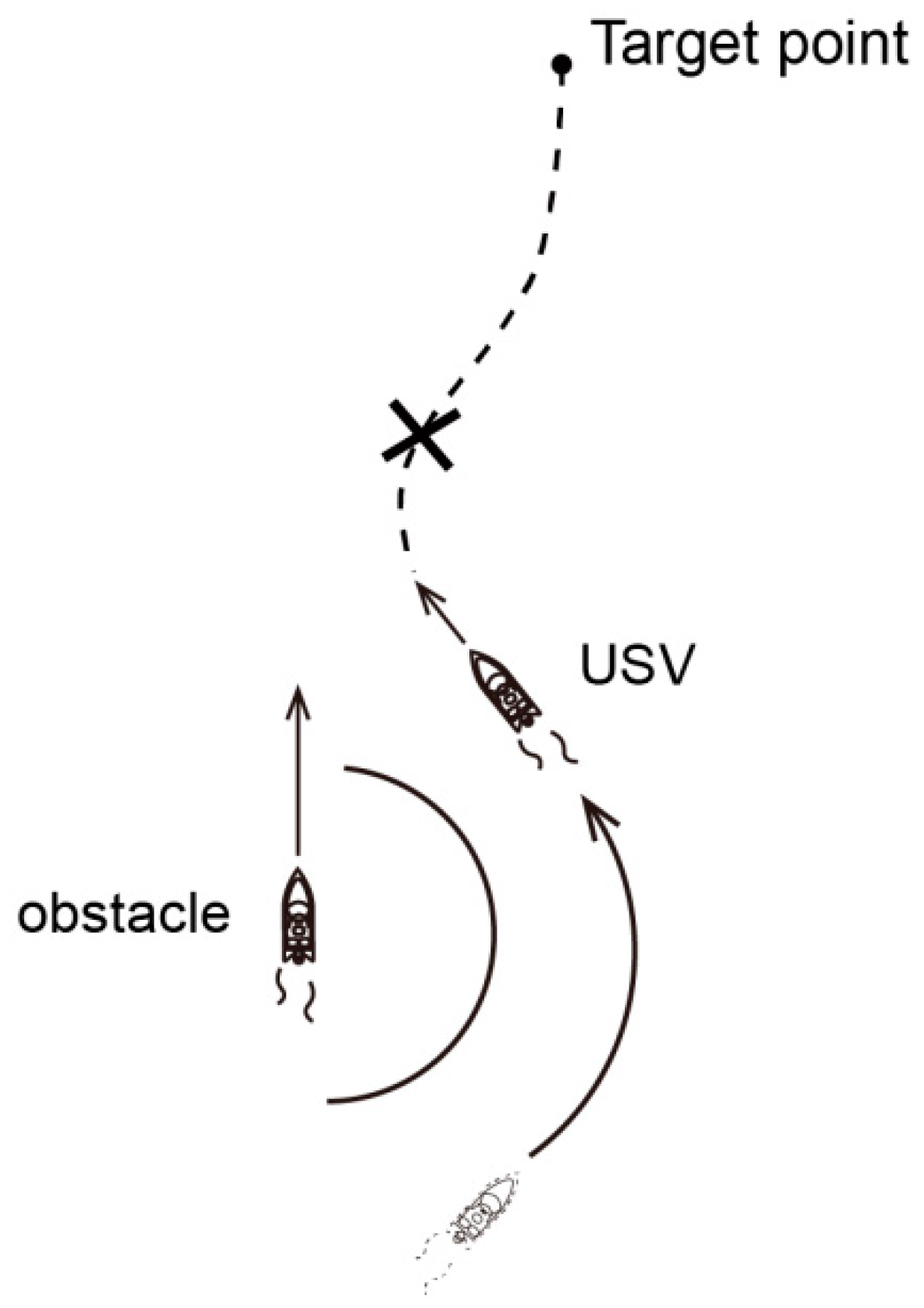
In our previous work, the aforementioned EIFDS algorithm exhibited outstanding obstacle avoidance capabilities in two-dimensional environments; however, it encounters a challenge known as the residual effect of interference (REI) post-avoidance, the disturbances induced by obstacle avoidance will continue to influence the initial flow field. The presence or absence of static obstacles may be disregarded, and dynamic obstacles present a different challenge. Particularly when the velocity vector of a dynamic obstacle converges with that of the SA, the risk evaluation index (REI) can lead to the proliferation of superfluous navigation routes and increased risks for SAs, as illustrated in Figure 2.

The presence of REI issues causes the SA to deviate from its optimal trajectory due to the influence of the obstacle’s REI. To mitigate this issue, a modification has been applied to Equation (5), as detailed below:

$$M_k=I-\kappa \left({\displaystyle \frac{n_k{n}_k^T}{{\left|{\mathsf{\Gamma }}_k\right|}^{1/{\rho }_k}{n}_k^T{n}_k}}+{\displaystyle \frac{\iota {\tau }_k{n}_k^T}{{\left|{\mathsf{\Gamma }}_k\right|}^{1/{\sigma }_k}{n}_k^T{n}_k{C}_k}}\right)-(\kappa -1)\left({\displaystyle \frac{{\alpha }_k{\alpha }_k^T}{{\left|{\mathsf{\Gamma }}_k\right|}^{1/{\rho }_{2_k}}{\alpha }_k^T{\alpha }_k}}\right)$$

(8)

In this equation, ${\displaystyle \frac{{\alpha }_k{\alpha }_k^T}{{\left|{\mathsf{\Gamma }}_k\right|}^{1/{\rho }_{2_k}}{\alpha }_k^T{\alpha }_k}}$ represents the modified disturbance matrix, ${\alpha }_k={\xi }_g-{\xi }_k={\left[\begin{array}{cc}{x}_g-x_k& y_g-y_k\end{array}\right]}^T$ denotes a vector that extends from the center point ${\xi }_k=(x_k,y_k)$ of the obstacle to the target point ${\xi }_g=(x_g,y_g)$, while $\rho 2_k$ signifies the post-disturbance coefficient applied to ${\rho }_k$ in an analogous manner. The position coefficient, denoted as $\kappa$, can be determined based on the relative positioning of SA with respect to the obstacle.

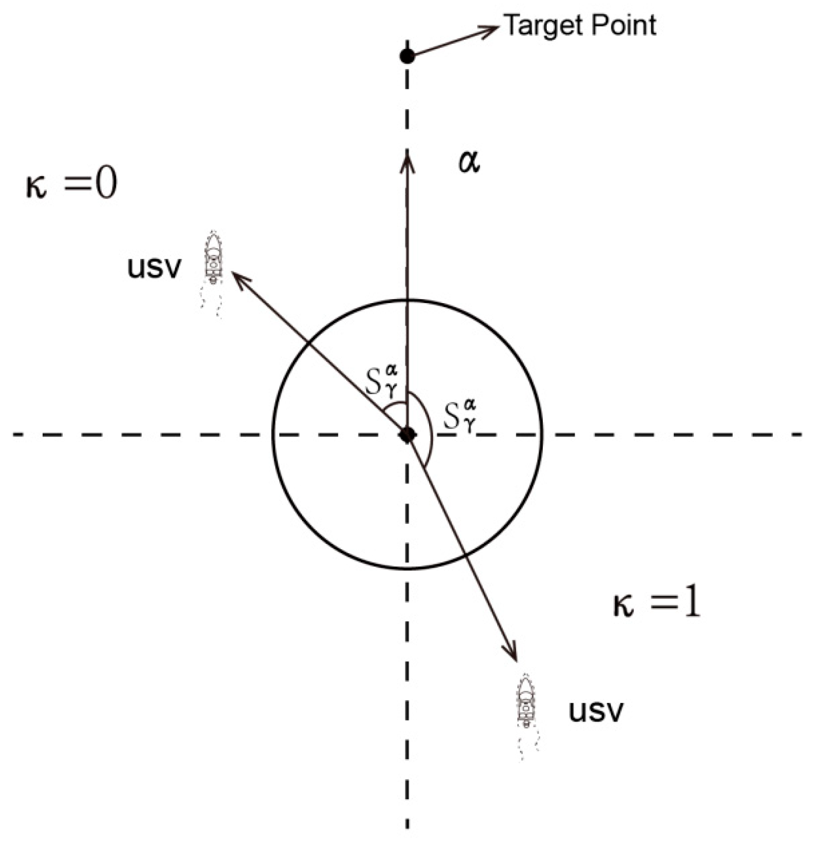
To ascertain the relative position of SA in relation to the obstacle, it is essential to compute the vector $r_k={\xi }_t-{\xi }_k={\left[\begin{array}{cc}{x}_t-x_k& y_t-y_k\end{array}\right]}^T$ originating from the center point of obstacle ${\xi }_k=(x_k,y_k)$ to the SA’s location ${\xi }_t=(x_t,y_t)$ at time $t$. Subsequently, the angle $S_{r_k}^{{\alpha }_k}$ between vector ${\alpha }_k$ and vector $r_k$ is determined, as illustrated in Figure 3.

① When the angle $S_{r_k}^{{\alpha }_k}<\pi /2$, the SA is positioned behind the obstacle, $\kappa =0$. Consequently, as indicated in Equation (8), the disturbance is represented by $M_k=I+{\displaystyle \frac{{\alpha }_k{\alpha }_k^T}{{\left|{\mathsf{\Gamma }}_k\right|}^{1/{\rho }_{2k}}{\alpha }_k^T{\alpha }_k}}$.

② When the angle $S_{r_k}^{{\alpha }_k}\ge \pi /2$, the SA is positioned before the obstacle, $\kappa =1$. Consequently, as indicated in Equation (8), the disturbance is represented by $M_k=I-{\displaystyle \frac{n_k{n}_k^T}{{\left|{\mathsf{\Gamma }}_k\right|}^{1/{\rho }_k}{n}_k^T{n}_k}}+{\displaystyle \frac{\iota {\tau }_k{n}_k^T}{{\left|{\mathsf{\Gamma }}_k\right|}^{1/{\sigma }_k}{n}_k^T{n}_k{C}_k}}$.

The adjustment of disturbance $M_k$ is contingent upon the relative positioning of the SA and surrounding obstacles, aimed at mitigating the REI issue induced by the EIFDS following obstacle avoidance maneuvers.

To assess feasibility, it is sufficient to confirm that the scenario (i.e., $\kappa =0$) under the condition of angle $S_{r_k}^{{\alpha }_k}<\pi /2$ being satisfied aligns with the navigation planning requirements, as angle $S_{r_k}^{{\alpha }_k}\ge \pi /2$ is consistent with the verified scenarios presented in Section 2.1 and Section 2.2.

① Initially, the trajectory must direct towards the designated target point:

Proof. 

When the distance between the SA and the obstacle is substantial, as this distance increases (${\mathsf{\Gamma }}_k\approx \infty$), the disturbance $M_k=I+{\displaystyle \frac{{\alpha }_k{\alpha }_k^T}{{\left|{\mathsf{\Gamma }}_k\right|}^{1/{\rho }_{2k}}{\alpha }_k^T{\alpha }_k}}$ converges towards $I$, resulting in a total flow field of ${\overline{u}}_t=I{u}_t=u_t$ that ultimately ensures the path heading reaches the target point. □

② Addressing the requirements for obstacle avoidance while eliminating REI.

Proof. 

At this moment, since the SA is positioned behind the obstacle, the disturbance can be characterized as $M_k=I+{\displaystyle \frac{{\alpha }_k{\alpha }_k^T}{{\left|{\mathsf{\Gamma }}_k\right|}^{1/{\rho }_{2k}}{\alpha }_k^T{\alpha }_k}}$. The direction of this disturbance emanates from the center of the obstacle towards the target point, aligning with a trajectory that moves away from the obstacle. Consequently, the initial flow field $u_t$ originating from the SA’s position to the target point also maintains a direction that diverges from the obstacle. Therefore, it can be concluded that the SA will not collide with the obstacle; additionally, at this juncture, there is no disturbance affecting the normal vector $n_k$ of the obstacle. Thus, the issue of REI induced by obstacles can be effectively addressed. A novel EIFDS algorithm for obstacle avoidance has been developed. □

3. The Challenge of Describing Obstacle Avoidance in Formation Control

Let us consider a scenario involving J surface agents (SAs), with the kinematic model for the jth SA articulated as follows:

$$\left\{\begin{array}{c}{\dot{x}}_j={\mu }_j\mathrm{c}\mathrm{o}\mathrm{s}{\psi }_j-v_j\mathrm{s}\mathrm{i}\mathrm{n}{\psi }_j\hfill \\ {\dot{y}}_j={\mu }_j\sin {\psi }_j+v_j\cos {\psi }_j\hfill \\ {\dot{\psi }}_j={\varphi }_j,\begin{array}{c} j=1,2,....,J\hfill \end{array}\end{array}\right.$$

(9)

In this equation, $x_j,y_j\in R$ denotes the position of the jth sensor agent (SA) within the terrestrial coordinate system; ${\psi }_j$ signifies the heading angle of the SA; ${\mu }_j$ and $v_j$ represents the magnitudes of the forwards and sideways velocity of the SA, respectively; ${\varphi }_j$ indicates the yaw rate of the SA; and J represents the total number of SA.

Each SA must ensure the maintenance of a safe distance ${\hslash }_k$ from obstacles to prevent potential collisions:

$$‖{\xi }_j-{\xi }_k‖>{\hslash }_k+R_k$$

(10)

Specifically, ${\xi }_k=(x_k,y_k)$ denotes the center point of the Kth obstacle, while $R_k$ signifies its radius. Consequently, the obstacle model can be derived from Equation (2) as follows:

$${\mathsf{\Gamma }}_k({\xi }_t)={({\displaystyle \frac{x_t-x_k}{{\hslash }_k+R_k}})}^2+{({\displaystyle \frac{y_t-y_k}{{\hslash }_k+R_k}})}^2$$

(11)

This formula is capable of constructing the boundary volume for a majority of obstacles; in cases involving particularly large obstacles, we can employ combinations of multiple obstacles.

Simultaneously, the members of the formation must maintain an appropriate distance ${\hslash }_j^{jj}$ from one another to mitigate the risk of collisions.

$$‖{\xi }_j-{\xi }_{jj}‖>{\hslash }_j^{jj}$$

(12)

In the equation, ${\xi }_{jj}=(x_{jj},y_{jj})$ denotes the location of the neighboring vessel.

4. A Strategy for Obstacle Avoidance in Formation Control

In contrast to the leader–follower approach, this study employs a virtual leader–follower methodology to enhance both the maneuverability and robustness of the formation. The position $P_O^F$ of the virtual leader within the Earth coordinate system is designated as the origin of the formation’s coordinate system, while the heading direction ${\psi }_{virl}$ of the virtual leader is defined as aligning with the X-axis of this formation coordinate framework. The position of the j-th SA in the Earth coordinate system is denoted as $P_j=[x_j;y_j]$, while its corresponding position in the coordinate system for formation analysis is represented as $P_j^F$. The relationship between these two positions can be articulated as follows:

$$P_j=P_O^F+\left[\begin{array}{cc}\cos {\psi }_t^{virl}& -\sin {\psi }_t^{virl}\\ \sin {\psi }_t^{virl}& \cos {\psi }_t^{virl}\end{array}\right]P_j^F$$

(13)

In this section, the motion trajectory of the virtual leader is governed by the second component of the EIFDS, with a constant velocity amplitude denoted as $V_{virl}$. The virtual leader exclusively accounts for static obstacles while navigating from the initial point to the target point of the formation task. Consequently, each follower’s designated position within the formation can be derived from that of the virtual leader. The EIFDS establishes a connection between the designated position and its corresponding follower. Given the inherent characteristics of EIFDS, it can be inferred that the follower will ultimately ‘flow’ towards the specific designated position within the formation due to streamline effects, thereby acquiring an enhanced capability to navigate around obstacles. To ensure that the follower converges to its designated position within the positions corresponding to the formation, the amplitude of the desired velocity $V=\sqrt{{\mu }^2+v^2}$ can be modulated to sustain the formation pattern of a fleet.

4.1. Navigation Strategies for Obstacle Avoidance

In accordance with the virtual leader and Equation (13), the designated position of the jth follower within the formation’s coordinate system is denoted as ${\xi }_{F_j}=(x_{F_j},y_{F_j})$, which serves as the target point for the previously mentioned EIFDS algorithm. Subsequently, Equation (1) is employed to establish the initial flow field. The initial flow field $u_j$ in the Earth coordinate system can be articulated as follows:

$$u_j={\left[\begin{array}{cc}{\displaystyle \frac{(x_{F_j}-x_j)}{\sqrt{{(x_{F_j}-x_j)}^2+{(y_{F_j}-y_j)}^2}}}& {\displaystyle \frac{(y_{F_j}-y_j)}{\sqrt{{(x_{F_j}-x_j)}^2+{(y_{F_j}-y_j)}^2}}}\end{array}\right]}^T$$

(14)

In the equation, ${\xi }_j=(x_j,y_j)$ denotes the position of the jth follower at this time.

In accordance with the EIFDS algorithm presented in Part II, the resultant value represents the disturbed flow velocity of the jth follower at this specific time:

$${\overline{u}}_j=\overline{M}(u_j-v_{\mathsf{\Gamma }})+v_{\mathsf{\Gamma }}={[\begin{array}{cc}{\overline{u}}_{jx}& {\overline{u}}_{jy}\end{array}]}^T$$

(15)

Consequently, the anticipated heading angle ${\psi }_{jd}=\arctan 2({\overline{u}}_{jy}/{\overline{u}}_{jx})$ of the follower at this moment is determined. Furthermore, the expected heading angle of the follower at any location within the terrestrial coordinate system can be derived from the aforementioned analysis.

The aforementioned results yield the anticipated heading angle ${\psi }_{jd}$ for the jth follower. To facilitate the convergence of the heading angle ${\psi }_j$ of the jth follower towards this expected value, a FTCLF is defined as follows:

$$L_j={‖{\psi }_j-{\psi }_{jd}‖}^2,j=1,....J$$

(16)

In order to regulate the heading angle ${\psi }_j$ to converge towards heading angle ${\psi }_{jd}$ within a specified time frame, the constraints of the FTCLF are delineated as follows [30]:

$$\begin{array}{cc}{\dot{L}}_j& =2e_{j\psi }({\varphi }_j-{\varphi }_{jd})\hfill \\ & \le {\omega }_j{L}_j-{\varsigma }_{j2}{L}_j^{1+1/{\mathcal{l}}_2}-{\varsigma }_{j3}{L}_j^{1-1/{\mathcal{l}}_2}\end{array}$$

(17)

Among these variables, ${\varsigma }_{j2},{\varsigma }_{j3}$ are positive constants. ${\mathcal{l}}_2>1$ and $e_{j\psi }$ denote the errors, while $e_{j\psi }={\psi }_j-{\psi }_{jd}$ and ${\omega }_j$ represent the relaxed variables that are subject to optimization, ${\varphi }_{jd}$ represents the expected yaw rate of the SA.

The quadratic programming of angular velocity, constrained by the FTCLF conditions, can be derived from Equation (17) as follows:

$$\begin{gathered} \underset{r_j,{\omega }_j}{\min }{\displaystyle \frac{1}{2}}({\varphi }_j^2+{\omega }_j^2)+l_{jr}{\omega }_j \\ s.t.\left\{\begin{array}{c}2e_{j\psi }({\varphi }_j-{\varphi }_{jd})\le {\omega }_j{L}_j-{\varsigma }_{j2}{L}_j^{1+1/{\mathcal{l}}_2}-{\varsigma }_{j3}{L}_j^{1-1/{\mathcal{l}}_2}\\ r_j\min \le r_j\le r_j\max \end{array}\right. \end{gathered}$$

(18)

$l_{jr}$ is the coefficient of the first-order term in the quadratic programming.

Proposition 1.

If the set $\Re =\left[{\varphi }_j\min ,{\varphi }_j\max \right]$ is non-empty, then for every $L_j>0$, the quadratic programming Equation (18) possesses a unique feasible solution.

Proof. 

For any arbitrary ${\overline{\varphi }}_j\in \Re$, we shall define

$${\overline{\omega }}_j={\displaystyle \frac{2e_{j\psi }({\overline{\varphi }}_j-{\varphi }_{jd})+{\varsigma }_{j2}{L}_j^{1+1/{\mathcal{l}}_2}+{\varsigma }_{j3}{L}_j^{1-1/{\mathcal{l}}_2}}{L_j}}$$

within the context of the equation $L_j\ne 0$. □

Among these, ${\overline{\varphi }}_j,{\overline{\omega }}_j$ meets the constraint conditions outlined in Equation (18), thereby ensuring the existence of a solution. Given that Equation (18) represents a complex quadratic programming problem and its domain is non-empty, it can be concluded that the solution is unique.

Through this process, we acquire the angular velocity signal of the follower at any given position within the Earth coordinate system.

4.2. Flow Field Structural Formation

To sustain the formation, the modulation of velocity amplitude is contingent upon the distance and bearing between the follower’s actual position and its designated location within the formation. The presence of external noise interference in real-world environments complicates the precise positioning of the follower by the actuator. To enhance both practicality and stability, it is deemed that the jth follower has successfully reached the designated position within the formation when it enters the range $R_j$ corresponding to this position, thereby fulfilling the convergence criteria.

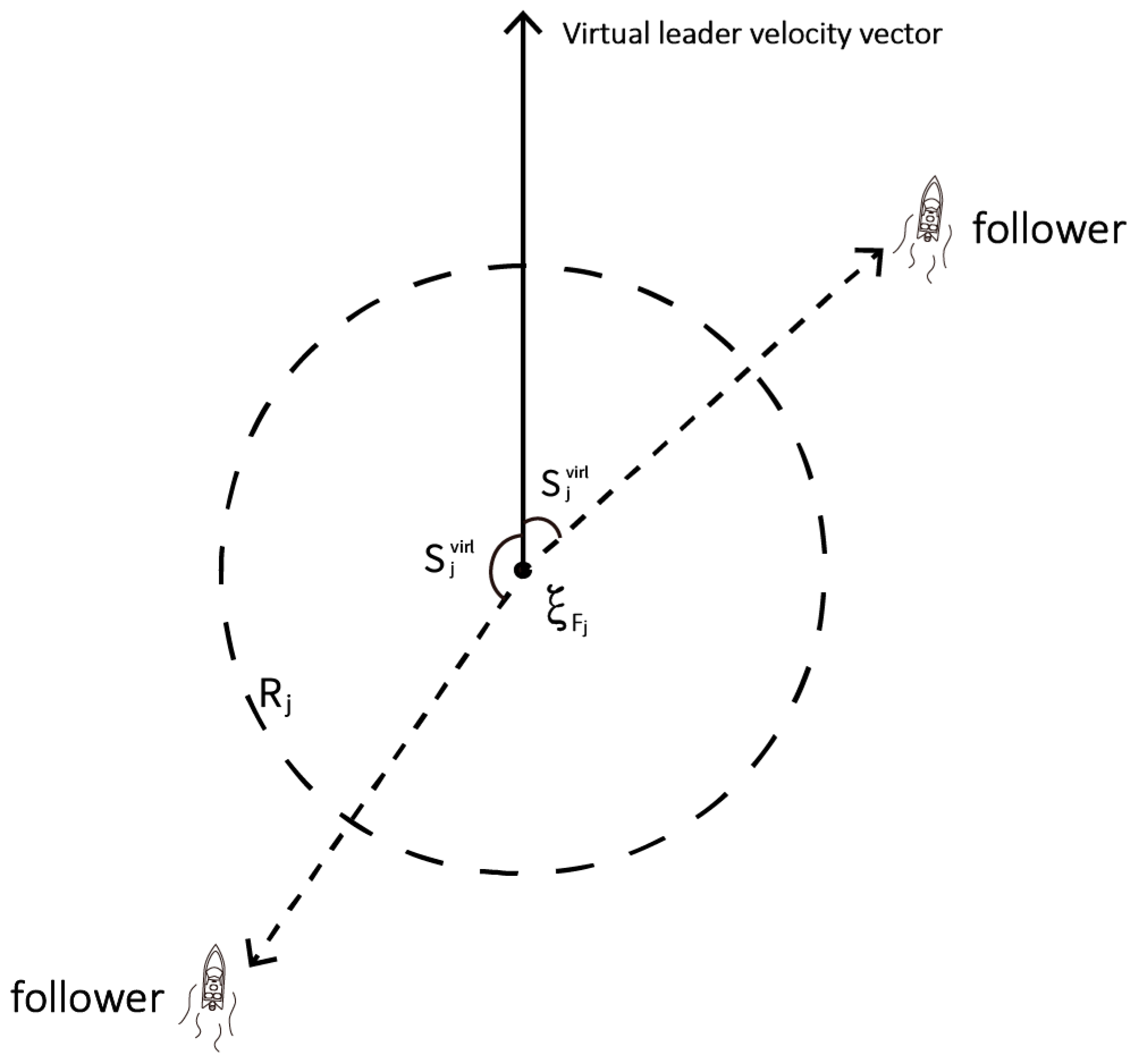
The design of velocity amplitude is categorized into two cases based on the orientation of the follower in relation to the specified position. Initially, the actual position of the follower is determined using Equation (13), alongside its corresponding designated position. The displacement vector $r_j={\xi }_j-{\xi }_{F_j}={\left[\begin{array}{cc}{x}_j-x_{F_j}& y_j-y_{F_j}\end{array}\right]}^T$, which represents the transition from the designated to the actual position of the follower, is then derived. Subsequently, we compute the angle $S_j^{virl}$ between this vector and the displacement vector associated with its corresponding position (i.e., representing the navigation direction of the virtual leader), as illustrated in Figure 4.

If $S_j^{virl}\ge {\displaystyle \frac{\pi }{2}}$, the follower is positioned behind the corresponding designated point; conversely, when angle $S_j^{virl}<{\displaystyle \frac{\pi }{2}}$, the follower occupies a position in front of this designated point. Based on these varying positions of the follower, distinct velocity strategies are formulated.

① When the angle $S_j^{virl}\ge {\displaystyle \frac{\pi }{2}}$, the follower operates in a pursuit state, with modifications made solely to the desired velocity amplitude $V_{jd}$ to facilitate its alignment with the designated position within the formation. The modulation of the target velocity amplitude $V_{jd}$ is predicated on the correlation between the actual distance from the follower to the designated position and the defined range $R_j$.

$$V_{jd}=\left\{\begin{array}{cc}{V}_{virl}+V_{{\omega }_j}(D_j^F-R_j)/\sqrt{(D_j^F-R_j{)}^2+{\mathrm{\Xi }}_j}& D_j^F\ge R_j\\ V_{virl}& D_j^F<R_j\end{array}\right.$$

(19)

In this equation, $V_{virl}$ denotes the velocity amplitude of the virtual leader, $D_j^F={‖r_j‖}^2$ signifies the distance between the follower’s actual position and its designated target, $R_j$ indicates the radius of the circular area encompassing the designated position range, while $V_{{\omega }_j}$ and ${\mathrm{\Xi }}_j$ are relaxation variables. Consequently, one can derive the velocity amplitude of the follower in a pursuit state.

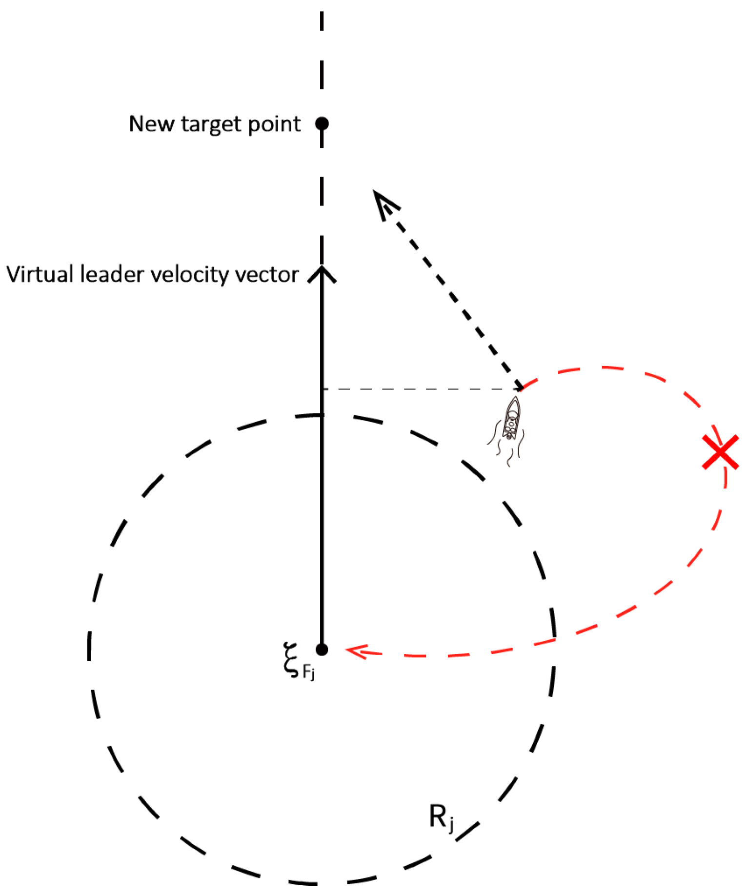
② When the angle $S_j^{virl}<{\displaystyle \frac{\pi }{2}}$, the follower is in an overshoot state, it becomes necessary not only to adjust the amplitude of the desired velocity $V_{jd}$ but also to make a slight modification to the heading angle. This adjustment facilitates improved convergence of the follower towards its designated position within the formation. Although guided by EIFDS, which ensures that the follower consistently ‘flows’ toward this target position, its overshoot state indicates that it has not yet reached this designated location. At this stage, the follower typically executes a significant angular deviation to reach the designated position, which is detrimental to the heading of the SA and should be avoided whenever possible, as illustrated in Figure 5.

To mitigate issues resulting from excessive maneuvering, it is essential to make slight adjustments to the heading angle and modify the target point while preserving the efficacy of obstacle avoidance. EIFDS has been modified from the originally designated position ${\xi }_{F_j}=(x_{F_j},y_{F_j})$ within the formation to a location along the displacement vector, specifically aligned with the virtual leader’s heading direction. This new target should be positioned at a distance of $2D_j^F\cos S_j^{Virl}$ (such that the actual position of follower ${\xi }_j=(x_j,y_j)$ relative to the designated position ${\xi }_{F_j}=(x_{F_j},y_{F_j})$ is twice the length of the projection of the distance between these two positions onto the displacement vector). This approach effectively addresses the issue of over-maneuvering resulting from an excessive number of states, thereby enhancing the robustness of the formation structure.

Subsequently, the amplitude of the velocity is fine-tuned while remaining in an overshoot state to facilitate the follower’s convergence to the designated position. The procedure for adjusting the velocity amplitude is outlined as follows:

$$V_{j{d}_{t+1}}=\left\{\begin{array}{cc}{V}_{j{d}_t}-C_F\mathrm{\Delta }T\hfill & V_{j_{t+1}}\ge V_{\mathrm{m}\mathrm{i}\mathrm{n}},D_j^F\ge R\\ \hspace{1em}{V}_{\mathrm{m}\mathrm{i}\mathrm{n}}\hfill & V_{j_{t+1}}<V_{\min },D_j^F\ge R_j\\ \hspace{1em}{V}_{virl}\hfill & D_j^F<R_j\end{array}\right.$$

(20)

In this equation, $V_{j{d}_t}$ and $V_{j{d}_{t+1}}$ denote the expected velocity amplitudes of the jth follower at time t and the subsequent time step, respectively; $\mathrm{\Delta }T$ signifies the observation duration; $C_F$ is associated with the relaxation variable $D_j^F$; and $V_{\min }$ represents the minimum velocity amplitude.

4.3. Strategies for Collision Avoidance Among Vessels

(1) Deficiencies in Inter-Vessel Collision Avoidance within the EIFDS Framework.

In the aforementioned formation structure, the utilization of EIFDS dictates the trajectory information of the virtual leader, thereby establishing the designated positions for each follower SA (denoted as j) within the formation. The j SAs function as followers and are linked to their respective designated positions through EIFDS. Owing to the inherent characteristics of EIFDS, these followers possess an intrinsic capability to ‘navigate towards’ their corresponding designated positions while also demonstrating proficiency in obstacle avoidance. To ensure the follower converges to the designated position, two state conditions—namely, the chasing state and overshoot state—were established for the velocity regulation scheme of the follower. The velocity amplitude is calibrated for the pursuit state to facilitate rapid convergence of the follower towards the designated position. To mitigate overshooting issues arising from an excessive number of states, the target point of EIFDS was adjusted, and the velocity amplitude was reduced to facilitate a more reasonable convergence of the follower towards the designated position. This ultimately enabled the formation strategy to be based on a flow field with obstacle avoidance capabilities, as illustrated in Figure 6.

The aforementioned description of the formation structure suggests that this formation strategy does not address collision avoidance among the vessels within the formation.

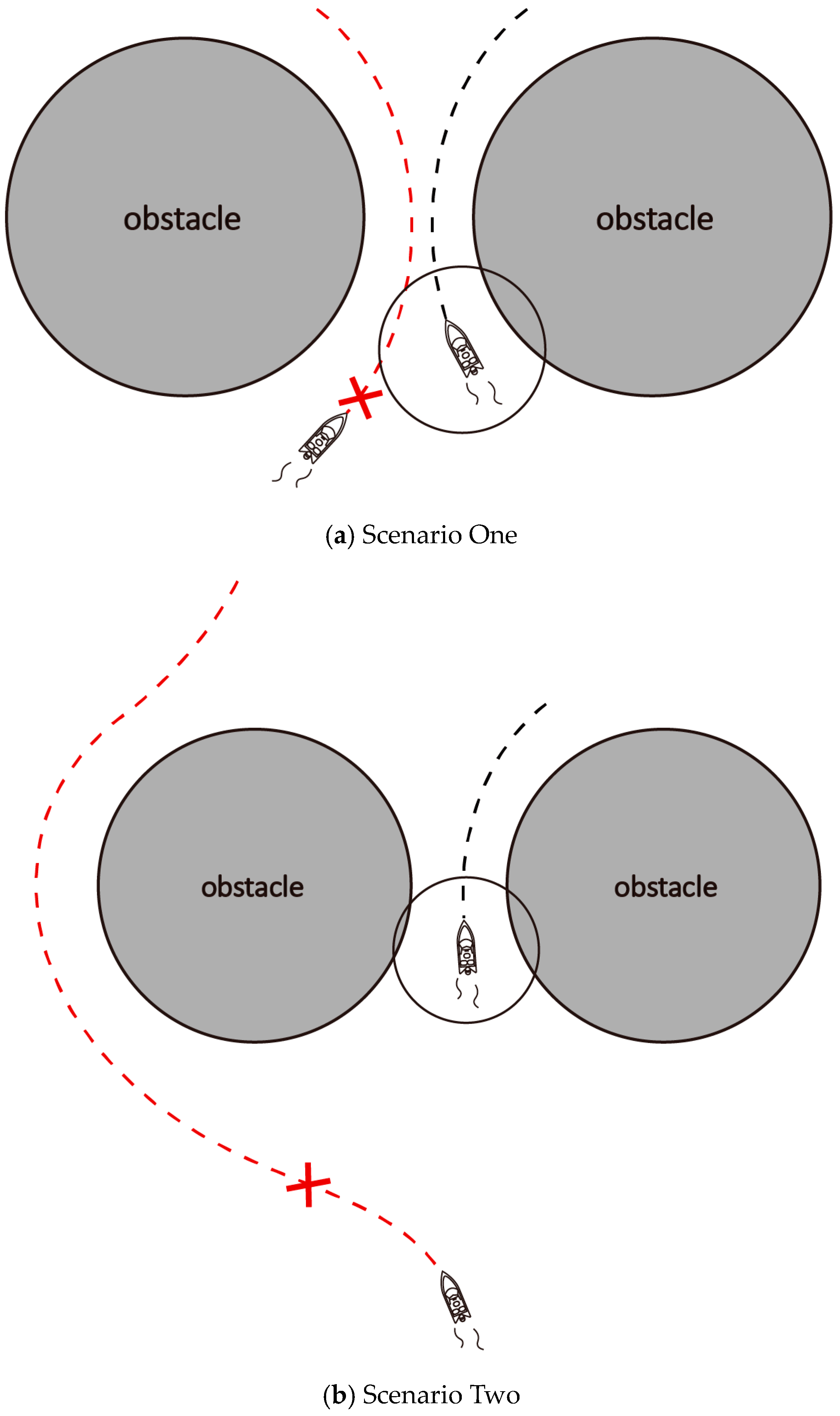
The problem arises due to adjacent boats as obstacles using the EIFDS method. This is primarily due to the fact that during convoy navigation, the navigational characteristics of vessels within a convoy—specifically their heading and velocity—are often similar. If the EIFDS approach remains in use for collision avoidance under these conditions, it may significantly complicate the flow field and exacerbate the challenges associated with obstacle avoidance, specifically, similar to barrier-type obstacles, as illustrated in Figure 7.

As illustrated in Figure 7a, when adjacent vessels within a convoy simultaneously navigate to circumvent a walled-type obstacle using EIFDS, there is a significant risk that one of the vessels may inadvertently enter the trap zone (at this juncture, the exponent in the obstacle weighting formula base is equal to zero), leading to potential failure in collision avoidance and resulting in collisions either between the vessels themselves or with the obstacle. As illustrated in Figure 7b, if one of the neighboring vessels first maneuvers to avoid the obstacle, subsequent vessels may deviate from the optimal route due to disturbances caused by this initial avoidance. This can lead to inefficient paths and significantly exacerbate the challenges associated with obstacle avoidance. Given the unique characteristics of convoy navigation, it is imperative to develop a novel collision avoidance strategy specifically tailored for boat-to-boat interactions. Additionally, to streamline the complexity of obstacle avoidance trajectories, it is essential to focus solely on optimizing the velocity amplitude $V$.

(2) The velocity amplitude FTCBF constraint is determined by the distance between the vessels and the time required for convergence.

The presence of EIFDS and fluid formation structures enables followers to maintain their formation while effectively avoiding obstacles. Nevertheless, a constraint on the safe distance between followers persists, which translates into a limitation on velocity amplitude to satisfy collision avoidance requirements for boats and establish a comprehensive strategy for collision avoidance within the formation.

Assuming that followers can effectively exchange state information within the range ${\hslash }_c$, we denote the jth follower as having a safety area ${\hslash }_j$ centered around itself. ${\hslash }_{jj}$ denotes a safety area of the adjacent follower. Consequently, the safety distance between this follower and its neighboring counterparts must satisfy:

$$‖{\xi }_j-{\xi }_{\mathrm{jj}}‖>{\hslash }_j+{\hslash }_{jj}={\hslash }_j^{jj}$$

(21)

To enhance computational efficiency and optimize fleet performance, $J$ followers are organized into hierarchical categories (i.e., secondary followers should refrain from interacting with primary followers). In this framework, the jth follower is assigned a lower priority compared to all other followers capable of exchanging states (this indicates that ${\mathrm{follower}}_{jj}>{\mathrm{follower}}_j$).

Let us define a control barrier function (CBF) as follows:

$$G_j^{jj}={‖{\xi }_j-{\xi }_{jj}‖}^2-{\hslash }_m^2,j,jj=1,\dots ,J(j\ne jj)$$

(22)

In the presented equation ${\hslash }_c\ge {\hslash }_m\ge {\hslash }_j^{jj}$, the secure set is defined as $G_j^{jj}\ge 0$.

$${\dot{G}}_j^{jj}=2V_j{z}_j^{jj}{\left[\begin{array}{cc}\cos {\psi }_j& \sin {\psi }_j\end{array}\right]}^T-2V_{jj}{z}_{jj}^j{\left[\begin{array}{cc}\cos {\psi }_{jj}& \sin {\psi }_{jj}\end{array}\right]}^T\ge -{\eta }_j^{jj}{G}_j^{jj}$$

(23)

Among these variables, ${\eta }_j^{jj}$ denotes the relaxed parameter that is subject to optimization.

Simultaneously, to facilitate the convergence of $G_j^{jj}<0$ towards the boundary of the secure set, a temporal constraint is introduced, thereby reformulating Equation (23) as follows:

$$\begin{array}{c}{\dot{G}}_j^{jj}=2V_j{z}_j^{jj}{\left[\begin{array}{cc}\mathrm{c}\mathrm{o}\mathrm{s}{\psi }_j& \mathrm{s}\mathrm{i}\mathrm{n}{\psi }_j\end{array}\right]}^T-2V_{jj}{z}_{jj}^j{\left[\begin{array}{cc}\mathrm{c}\mathrm{o}\mathrm{S}{\psi }_{jj}& \mathrm{s}\mathrm{i}\mathrm{n}{\psi }_{jj}\end{array}\right]}^T\\ \hspace{1em}\hspace{1em}\ge -{\eta }_j^{jj}{G}_j^{jj}+{\varsigma }_j^{jj}\mathrm{m}\mathrm{i}\mathrm{n}{\left\{0,G_j^{jj}\right\}}^{1+1/{\mathcal{l}}_j^{jj}}+{\varsigma }_j^{jj}\mathrm{m}\mathrm{i}\mathrm{n}{\left\{0,G_j^{jj}\right\}}^{1-1/{\mathcal{l}}_j^{jj}}\end{array}$$

(24)

In the presented equation ${\varsigma }_j^{jj}>0$, ${\mathcal{l}}_j^{jj}>1$.

From this, an FTCBF constraint is derived. Subsequently, a quadratic programming controller is developed to determine the final velocity amplitude signal.

To achieve the desired velocity amplitude $V_{jd}$ convergence, maintain formation integrity, and ensure a safe distance between vessels, we employ the following quadratic programming approach with FTCBF constraints for velocity amplitude optimization:

$$\begin{gathered} \underset{V_j,{\eta }_j^{jj}}{\mathrm{m}\mathrm{i}\mathrm{n}}{\displaystyle \frac{1}{2}}{(V_j-V_{jd})}^2+{\displaystyle \sum _{jj=1,jj\ne j}^J(\frac{1}{2}{\eta }_j^{j{j}^2}}+l_{jV}{\eta }_j^{jj}), \\ s.t.\left\{\begin{array}{c}{\dot{G}}_j^{jj}\ge -{\eta }_j^{jj}{G}_j^{jj}+{\varsigma }_j^{jj}\mathrm{m}\mathrm{i}\mathrm{n}{\left\{0,G_j^{jj}\right\}}^{1+1/{\mathcal{l}}_j^{jj}}+{\varsigma }_j^{jj}\mathrm{m}\mathrm{i}\mathrm{n}{\left\{0,G_j^{jj}\right\}}^{1-1/{\mathcal{l}}_j^{jj}}\\ V_{j\mathrm{m}\mathrm{i}\mathrm{n}}\le V_j\le V_{j\mathrm{m}\mathrm{i}\mathrm{n}}\end{array}\right. \end{gathered}$$

(25)

In this equation, $V_{j\mathrm{m}\mathrm{a}\mathrm{x}},V_{j\mathrm{m}\mathrm{i}\mathrm{n}}$ denote the maximum and minimum velocity amplitudes, respectively, while $l^{jV}$ represents the relaxation variable.

Ultimately, by resolving Equation (25), the final velocity amplitude signal can be derived to satisfy the formation velocity amplitude criteria outlined in Section 4.2 and the inter-boat distance constraints specified in Equation (21).

4.4. Summary of the Process

The subsequent outline delineates the decision-making process for formation in the aforementioned scenario.

① By employing EIDFS and a constant velocity amplitude, the virtual leader is directed towards the mission’s destination. This virtual leader is capable of generating the specified positions for each SA within the formation.

② Guided by the EIFDS streamline, the anticipated heading angle of each SA at any given position is determined, directing the formation towards the designated location of its corresponding member while endowing it with obstacle avoidance capabilities. Ultimately, the angular velocity signal of the SA at this juncture is derived through a quadratic programming solution constrained by FTCLF.

③ Utilizing the fluid formation strategy, the velocity amplitude is adjusted during the pursuit state, while both the velocity amplitude and the EIFDS target point are meticulously fine-tuned in the overshoot state. Consequently, the anticipated velocity amplitude of SA can be derived at this juncture.

④ Based on the desired velocity amplitude, the velocity amplitude is regulated by FTCBF in accordance with the inter-vessel distance, and an optimal velocity amplitude signal is derived through quadratic programming. Ultimately, a guidance strategy for SAs to maintain formation and navigate around obstacles is established.

5. Simulation Techniques

This section will present the simulation results to validate the efficacy of the method discussed in this paper.

5.1. Comparison of REI Problems

The EIFDS, in contrast to interfered fluid dynamical system (IFDS), provides an effective solution to the REI problem:

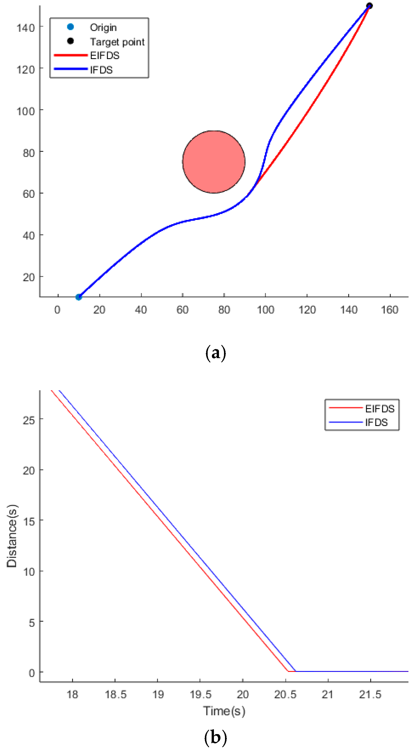
The initial position of the SA is established at coordinates (10, 10), with the target point located at coordinates (150, 150). The path encounters an obstacle whose center is situated at coordinates (75, 75) and possesses a radius of 15 m, as illustrated in Figure 8a. The velocity amplitude $V$ of the SA is maintained at a constant value 10 m/s, while the heading angle is established at 45 degrees.

In this scenario, to streamline the variables, the two-dimensional IFDS is incorporated into the deviation matrix. The disturbance coefficient of the IFDS, denoted as ${\rho }_k$, is established at 3, while the deviation coefficient of the IFDS, represented as ${\sigma }_k$, is set at 2. The disturbance coefficient ${\rho }_k$ of the EIFDS is established at 3, the deviation coefficient ${\sigma }_k$ is set to 2, and the post-disturbance coefficient $\rho 2_k$ is defined as 2. 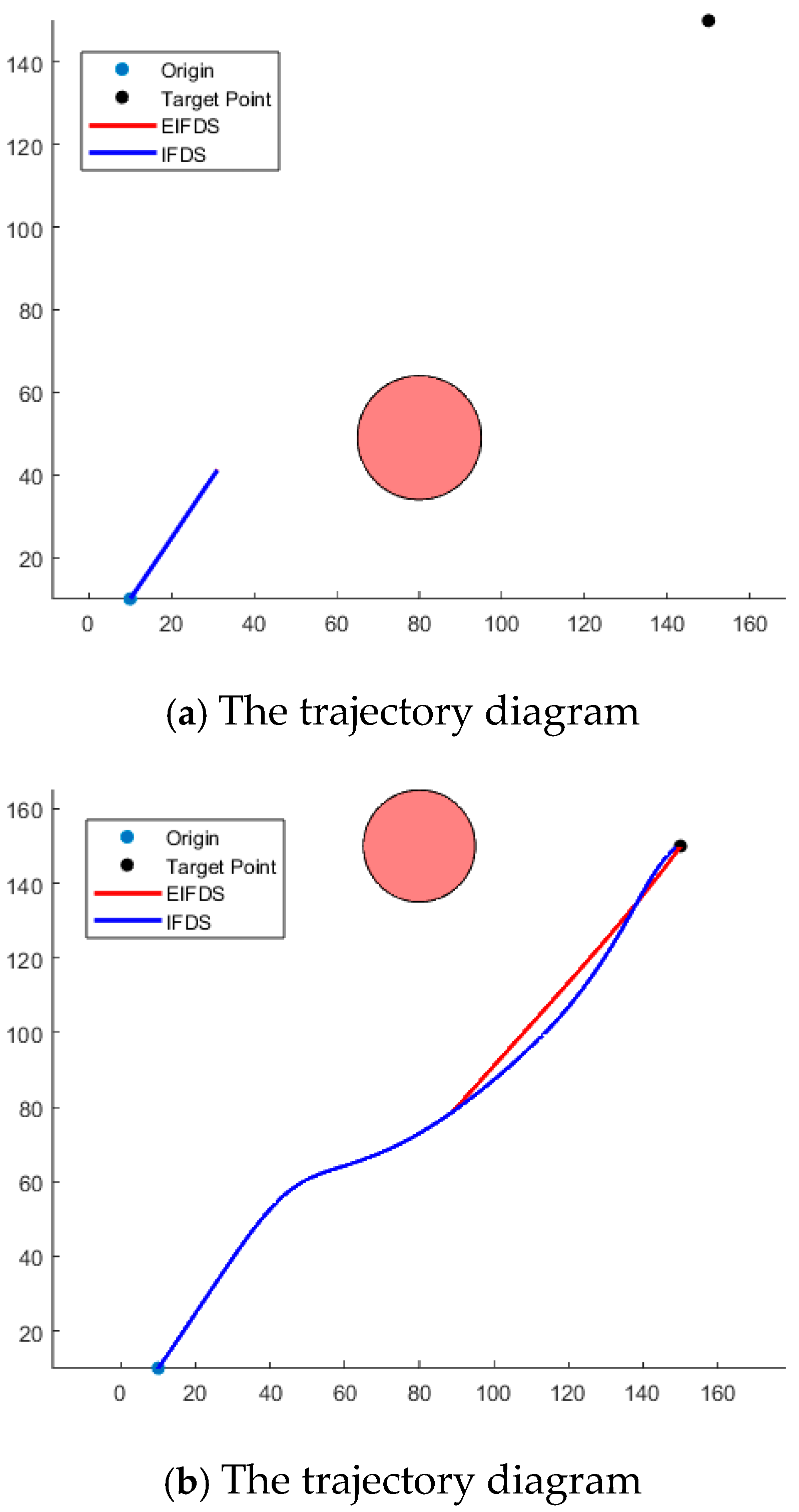It is evident that EIFDS is not constrained by the REI problem; furthermore, as illustrated in Figure 8b, EIFDS achieves convergence to the target point more rapidly. Next, a dynamic obstacle scenario will be developed to assess the superiority of EIFDS over IFDS. The starting position of the SA is established at coordinates (10, 10), with the target point located at coordinates (150, 150). Within this path, a dynamic obstacle is introduced, originating from coordinates (80, 0) and possessing a radius of 15 m. This obstacle travels along the Y-axis at a constant velocity of 12 m/s, as illustrated in Figure 9. Additionally, the velocity amplitude of SA is maintained at a constant value denoted as 10 m/s, while its heading angle is initially set to 45 degrees.

As illustrated in Figure 9a,b, the scenario remains consistent with previous observations, where the disturbance coefficient ${\rho }_k$ of the IFDS is set to 3 and the deviation coefficient ${\sigma }_k$ is established at 2. In contrast, for the EIFDS, the disturbance coefficient ${\rho }_k$ is also set to 3, while its deviation coefficient ${\sigma }_k$ is maintained at 2, alongside a post-disturbance coefficient $\rho 2_k$ fixed at 2. It is evident that EIFDS is not constrained by the REI problem, whereas the REI issue in IFDS becomes more pronounced in the presence of dynamic obstacles.

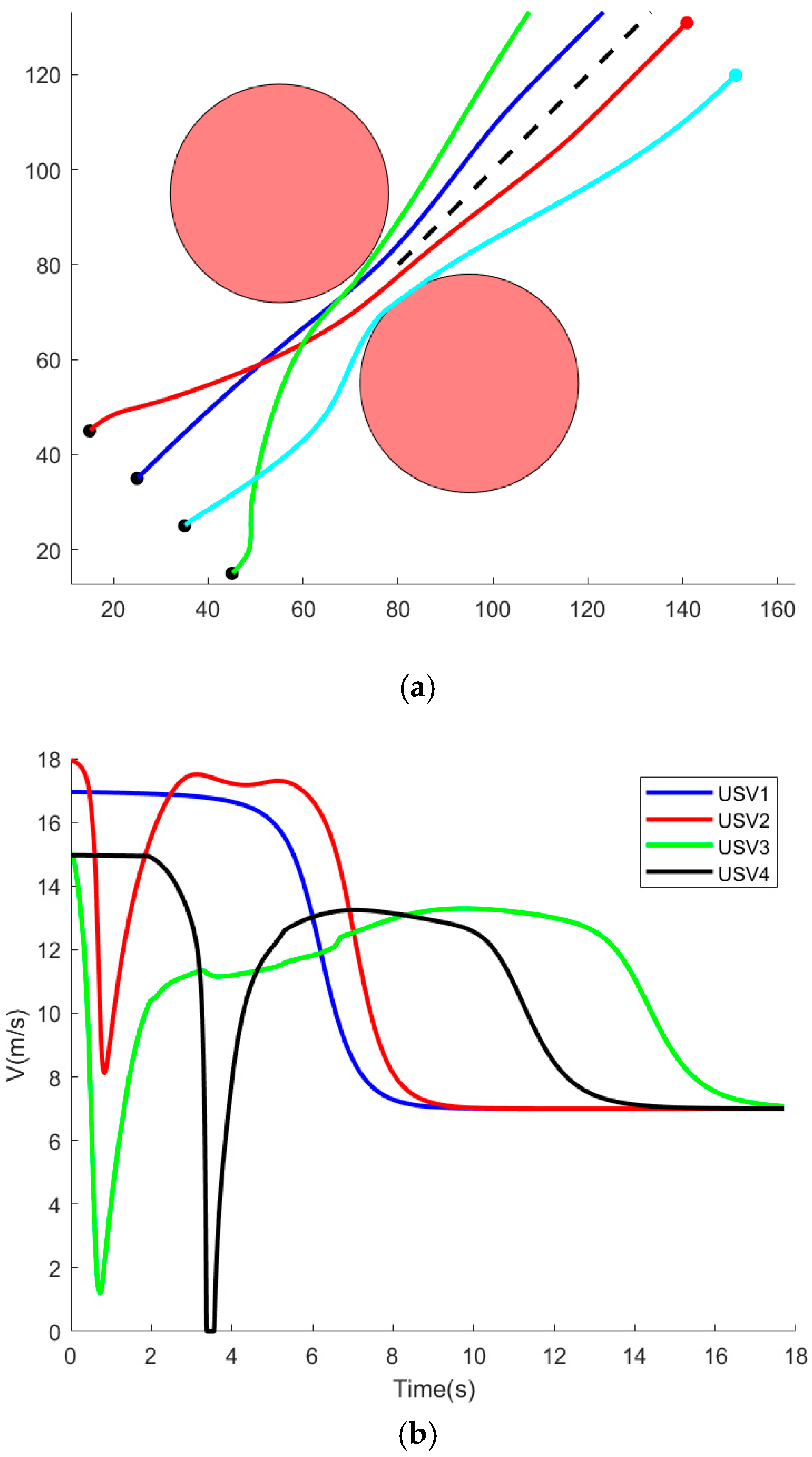
5.2. Multi-Obstacle Formation and Obstacle Avoidance Strategies

To assess the capability of formation obstacle avoidance and the subsequent regrouping ability post-avoidance, the simulation design environment is outlined as follows:

Within the framework of the geodetic coordinate system, the virtual leader is initially positioned at (50, 50). The amplitude of the virtual leader’s velocity, denoted as AAA, is set at 7 m/s. The parameters of EIFDS for the virtual leader are individually configured: the disturbance coefficient ${\rho }_k$ is set to 3, the deviation coefficient ${\sigma }_k$ to 2, and the post-disturbance coefficient $\rho 2_k$ also to 2. The designated positions for each SA within the formation coordinate system are as follows: SA1 at (−15, 0), SA2 at (−30, 0), SA3 at (−15, 15), and SA4 at (−15, −15).

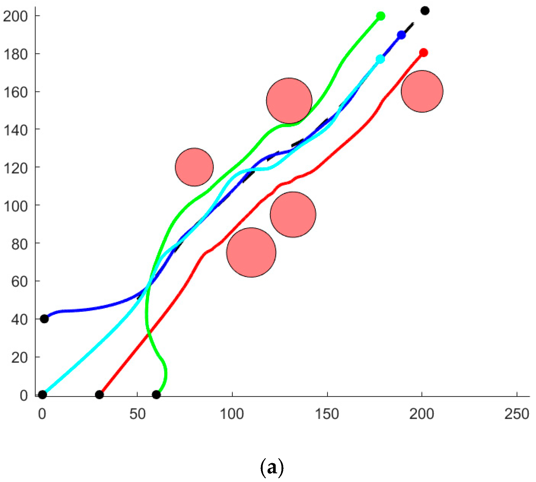
In a specified area, four SA units are distributed with their initial positions and heading angles defined in the geodetic coordinate system as follows: SA1(1, 40, 45°), SA2(30, 0, 45°), SA3(60, 0, 45°), and SA4(0, 0, 45°). The minimum velocity amplitude $V_{\min }$ for all units is set at 1 m/s. The maximum velocity amplitudes $V_{\max }$ are recorded as 17 m/s for SA1, 18 m/s for SA2, 16 m/s for SA3, and 15 m/s for SA4. The angular velocity interval $\Re =\left[r_j\min =-1,r_j\max =1\right]$ is expressed in radians per second; ${\varsigma }_{j2}={\varsigma }_{j3}=5,{\varsigma }_j^{jj}=8$. The relaxation variable ${\mathrm{\Xi }}_j$ is 36; the coefficient of the angular velocity quadratic term $l_{jr}$ within the linear component of the quadratic programming problem is designated as 0.1; the fixed time exponential parameters ${\mathcal{l}}_{j2},{\mathcal{l}}_j^{jj}$ are uniformly set to 2 for all instances; the coefficient of the velocity amplitude quadratic term $l_{jV}$ in the linear aspect of the quadratic programming problem is also specified as 0.1; regarding EIFDS parameters, for the SA, the disturbance coefficient ${\rho }_k$ is assigned a value of 3, while the deviation coefficient ${\sigma }_k$ and post-disturbance coefficient $\rho 2_k$ are both set to 2. The prioritization of SAs is established as SA1 > SA2 > SA4 > SA3, with a designated safety distance of 10 m maintained between formation members. The obstacles are positioned at coordinates (110, 75), (130, 155), (200, 160), (80, 120), and (132, 95), each characterized by radii of 13 m, 12 m, 11 m, 10 m, and 12 m, respectively. The results from the simulation are presented next.

As illustrated in Figure 10a, all members of the formation successfully navigated obstacles, ultimately achieving the desired formation pattern. Figure 10b presents the velocity amplitude output signals for each SA under the streamline formation structure and FTCBF constraints. Meanwhile, Figure 10c displays the angular velocity output signals for each SA subjected to EIFDS and FTCLF constraints. 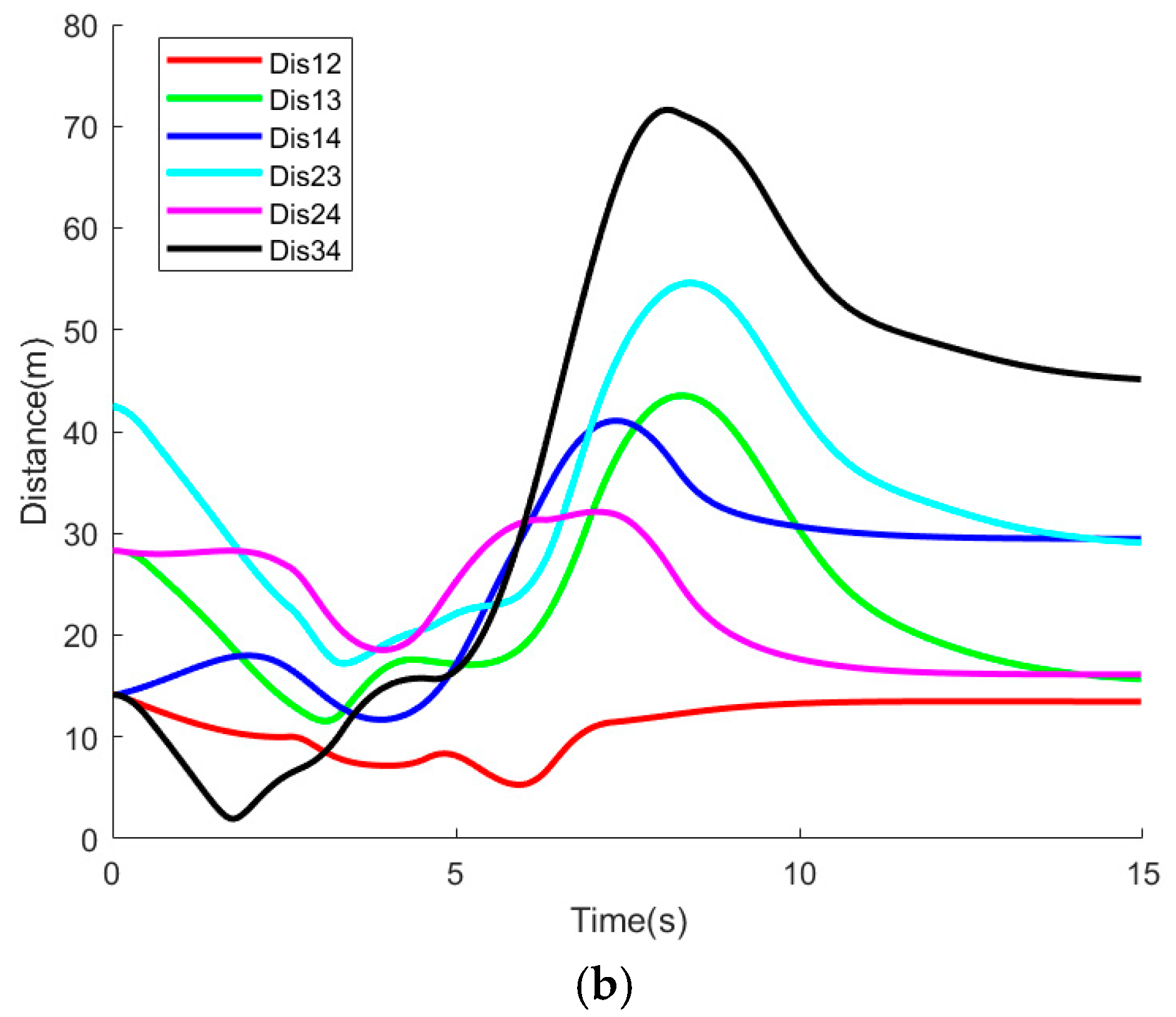Figure 10d illustrates the inter-member distances within the formation, demonstrating that under the FTCBF constraint, members maintain a separation exceeding 10 m. This observation underscores the efficacy of the quadratic programming controller and confirms that no collisions occur among formation members.

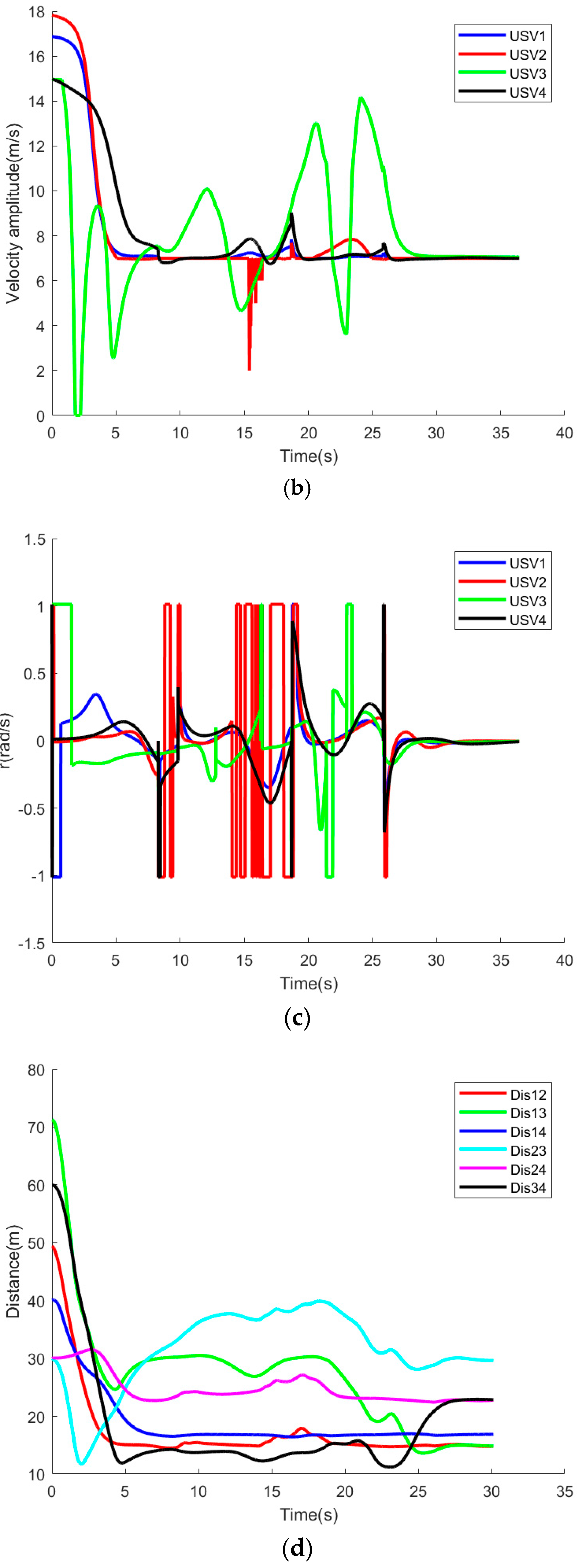
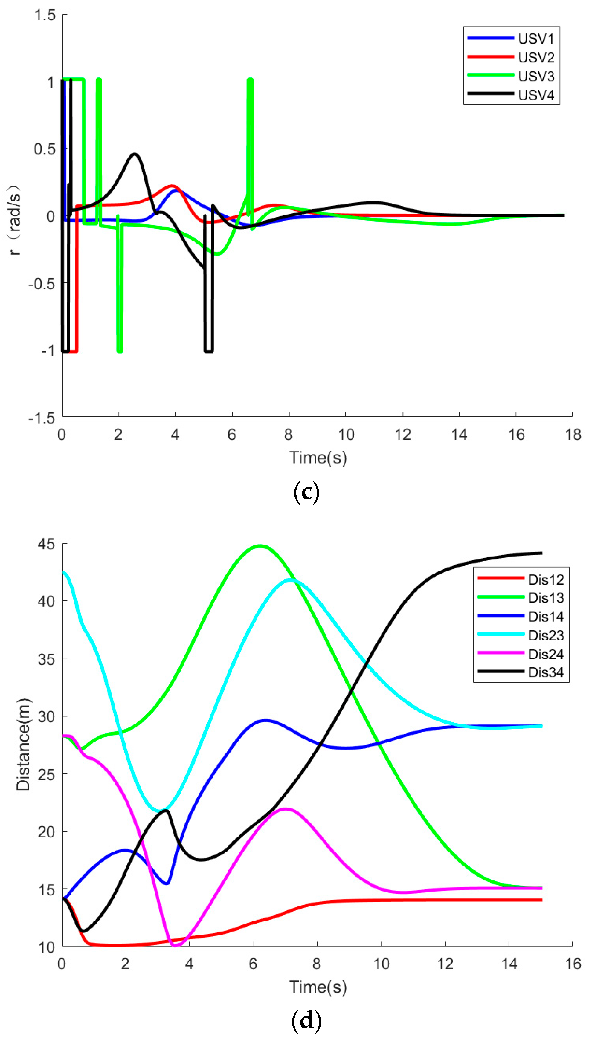
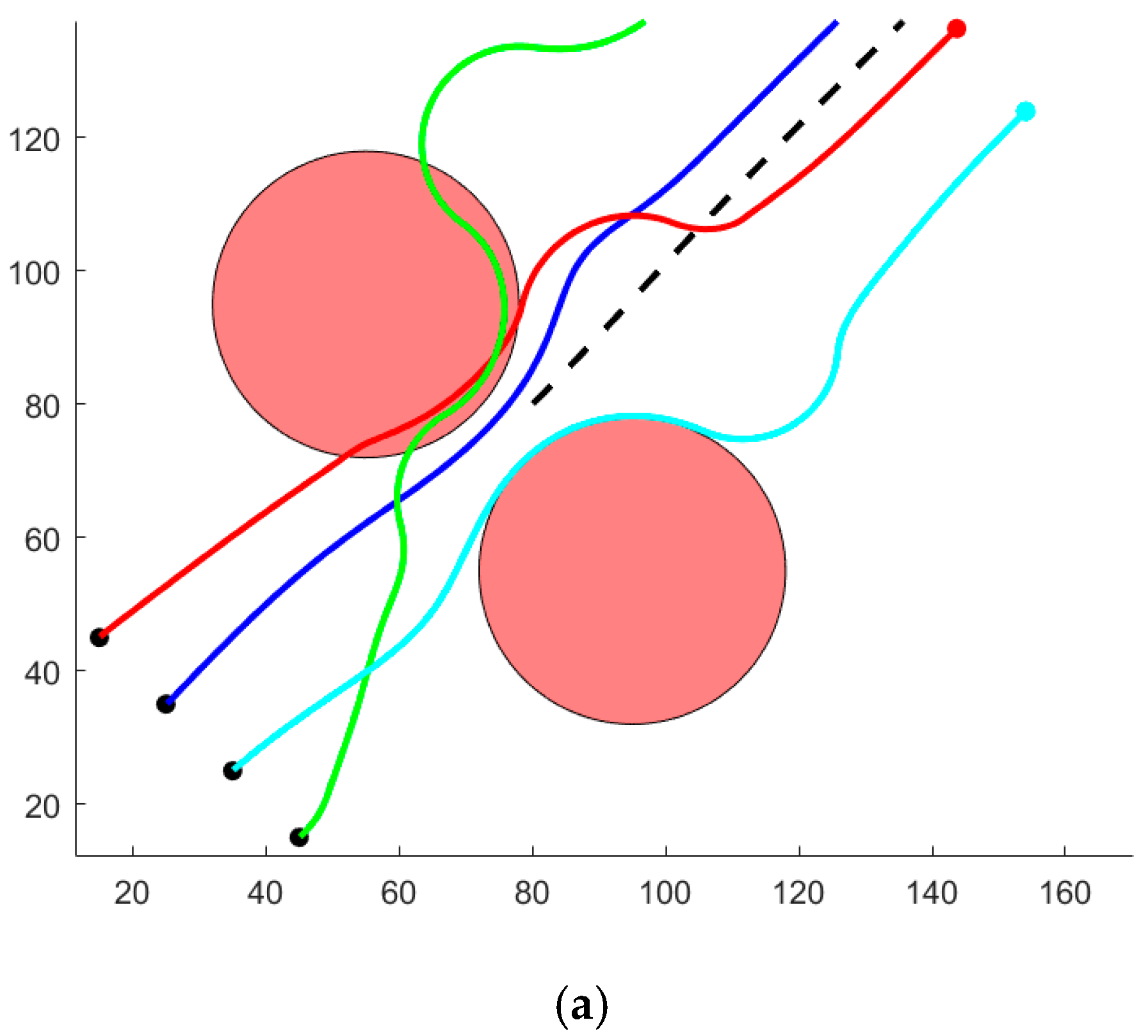
5.3. Formation Obstacle Avoidance in Wall Barrier Environments

To assess the efficacy of the proposed formation’s obstacle avoidance strategy, a comparative analysis is conducted between the decision-making framework presented in this paper and that of the IFDS formation when confronted with a barrier obstacle. The simulation design environment is outlined as follows:

The initial position of the virtual leader within the Earth coordinate system is defined as (80, 80). The amplitude of the virtual leader’s velocity, denoted as $V_{virl}$ is set at 7 m/s. The parameters for EIFDS governing the virtual leader are individually specified: the disturbance coefficient ${\rho }_k$ is established at 3, the deviation coefficient ${\sigma }_k$ is assigned a value of 2, and the post-disturbance coefficient $\rho 2_k$ is also designated as 2. Furthermore, in the formation coordinate system, each SA has predetermined positions: SA1(−7, 7), SA2(−7, −7), SA3(−7, 22), and SA4(−7, −22).

Four SAs are arranged linearly within a specified area, with their initial positions and heading angles defined in the geodetic coordinate system as follows: SA1(15, 45, 45°), SA2(25, 35, 45°), SA3(35, 25, 45°), and SA4(45, 15, 45°). The minimum velocity amplitude $V_{\min }$ for all units is set at 0.1 m/s; the maximum velocity amplitudes $V_{\max }$ are recorded as 17 m/s for SA1, 18 m/s for SA2, 16 m/s for SA3, and 15 m/s for SA4. The angular velocity interval $\Re =\left[r_j\min =-1,r_j\max =1\right]$ is expressed in radians per second;${\varsigma }_{j2}={\varsigma }_{j3}=5,{\varsigma }_j^{jj}=8$. The relaxation variable ${\mathrm{\Xi }}_j$ is 36. In the context of quadratic programming, the linear coefficient associated with the quadratic term of angular velocity $l_{jr}$ is set to 0.1. Additionally, the fixed time exponential parameters ${\mathcal{l}}_{j2},{\mathcal{l}}_j^{jj}$ are uniformly assigned a value of 2 across all instances. Similarly, the linear coefficient for the quadratic term $l_{jV}$ related to velocity magnitude in quadratic programming also holds a value of 0.1. Regarding EIFDS parameters for SA, the disturbance coefficient ${\rho }_k$ is designated as 3, while the deviation coefficient ${\sigma }_k$ and post-disturbance coefficient $\rho 2_k$ are both set to 2. The prioritization of the SA is as follows: SA1 > SA2 > SA4 > SA3, with a safety distance of 10 m maintained between formation members. The obstacles are positioned at coordinates (55, 95) and (95, 55), each with a radius of 23 m. The results from the simulation are presented below.

To assess the efficacy of the formation’s obstacle avoidance capabilities, a decision-making framework for IFDS formation obstacle avoidance was developed for comparative analysis. To maintain variable uniqueness, both the formation structure and parameters align with those presented in this study, while environmental factors and performance metrics for each vessel remain consistent (i.e., initial state, velocity amplitude constraints, and angular velocity constraints are uniform). In light of these conditions, the IFDS parameters for each SA have been established, with the disturbance coefficient ${\rho }_k$ set to 3 and the deviation coefficient ${\sigma }_k$ set to 2. The prioritization of SAs is as follows: SA1 > SA2 > SA4 > SA3. A safety distance of 10 m is maintained between formation members. The simulation results are presented below.

The simulation results presented above, particularly in Figure 11a and Figure 12a, demonstrate that all members of the formation successfully navigated around obstacles as per the avoidance strategy proposed in this paper, ultimately achieving a formation. In the context of IFDS formation obstacle avoidance, the constraints of a minimum inter-barrier distance of 10 m and a safe inter-boat distance of 10 m can easily lead to the emergence of a sudden trap area during navigation, potentially resulting in the failure of the SA to evade obstacles in a timely manner. As illustrated in Figure 11d and Figure 12b, the formation avoidance strategy proposed in this study, under the constraints of FTCBF, successfully maintains a separation distance exceeding 10 m among its members. This finding underscores the efficacy of the quadratic programming controller and confirms that no collisions occur between formation members. Nevertheless, in the context of IFDS formation avoidance, the presence of chaotic dynamics, REI issues, and the sudden emergence of trap zones within the flow field beneath barrier obstacles in a two-dimensional environment impede members from maintaining a safe inter-member distance. Figure 11b illustrates the velocity amplitude output signals of each SA under the formation avoidance strategy proposed in this study. Figure 11c presents the angular velocity output signals of each SA within the same framework. Consequently, a comparative analysis of these data substantiates the efficacy of this formation avoidance strategy.

6. Conclusions

This study presents a fixed-time streamline traction formation avoidance strategy for a fleet of vehicles navigating around obstacles. The formation structure is established based on the leader–follower approach, wherein a virtual leader is directed towards the target point of the formation task utilizing the EIFDS tractor. The designated positions for each member within the formation are determined by this virtual leader. Subsequently, both the SA and their corresponding designated positions are interconnected through the EIFDS. Owing to the inherent characteristics of the EIFDS, the SA consistently navigates towards its designated location while exhibiting obstacle avoidance capabilities, thus establishing its anticipated trajectory. To ensure the stability of the formation, a comprehensive approach utilizing flow field methodologies was employed to design the SA velocity amplitude under varying conditions, thereby determining the anticipated SA velocity amplitude accordingly. In addressing the challenge of preventing collisions between vessels, employing FTCBF to regulate velocity amplitude can effectively maintain a safe distance between boats. An FTCLF is employed to impose the angular velocity constraint, subsequently yielding the outputs of angular velocity and velocity amplitude through a quadratic programming controller. The effectiveness and superiority of the formation obstacle avoidance strategy proposed in this paper were validated through simulations of obstacle avoidance and comparative analysis with barrier obstacles.

In conclusion, this method offers novel theoretical support for the practical application of SA formation obstacle avoidance. However, in this paper, corresponding dynamic constraints have not been established, and the influences brought by environmental noises such as wind and waves and sea clutter have not been taken into account. It is merely based on the decision-making level of formation path planning. This might have an impact on the feasibility of SAs in the actual process of formation obstacle avoidance. In the future, based on the inspiration from MFC, a new predictive control algorithm will be devised to adjust the parameters in the EIFDS obstacle avoidance algorithm, so as to meet the dynamic constraints of SAs and deal with environmental noise. This will further decrease the need for parameter adjustment, enhance the autonomy of SA formation, and ensure its feasibility in practical environments.