An Offline Reinforcement Learning Approach for Path Following of an Unmanned Surface Vehicle

Abstract

Path following is crucial for enhancing the autonomy of unmanned surface vehicles (USVs) in water monitoring missions. This paper presents an offline reinforcement learning (RL) controller for USVs. The controller employs the soft actor–critic algorithm with a diversified Q-ensemble to optimize the steering control policy using a pre-collected dataset of USV path-following trials. A Markov decision process (MDP) tailored for path following is formulated. The proposed offline RL steering controller, trained on static datasets, demonstrates improved sample efficiency and asymptotic performance due to an expanded ensemble of Q-networks. The accuracy and adaptive learning capabilities of the RL controller are validated through simulations and free-running tests.

1. Introduction

As concerns about marine resource exploitation and maritime rights escalate, the demand for intelligent control and autonomous navigation in marine vessels is steadily growing. Path following, encompassing navigation, guidance, control, and actuation, is pivotal for enabling autonomous travel. Accurate tracking of predefined waypoints is crucial to ensure safety.

Designing efficient control systems for underactuated marine vessels poses several challenges, including developing mathematical models that accurately capture complex vehicle dynamics and environmental disturbances. To tackle these, various control algorithms have been devised and tested through simulations and field trials, such as proportional–integral–derivative (PID) control [1], fuzzy control [2], adaptive control, and nonlinear model predictive control (NMPC) [3]. Further research in control engineering has focused on enhancing performance by utilizing parameter estimation and system identification techniques to learn the unmanned surface vehicle (USV) model and its parameters.

However, model-based controllers often rely heavily on prior system knowledge, limiting their robustness against disturbances and modeling uncertainties. To overcome these limitations, self-learning approaches have been proposed that do not require prior knowledge of USV dynamics for controller design or parameter tuning.

Certain neural networks are designed to approximate model nonlinearities and disturbances, enhancing robustness against uncertainties [4]. Other studies concentrate on backpropagation (BP) [5] or self-learning policies to update parameters in PID [6] or NMPC controllers [7].

In recent years, deep reinforcement learning (DRL) algorithms have demonstrated remarkable success across various domains, including robotics [8], autonomous vehicles [9], unmanned aerial vehicles (UAVs) [10], and USVs [11]. Researchers have independently applied model-free online RL algorithms to design self-learning controllers for tasks such as path following [12], formation control [13], path planning [14], and collision avoidance [15].

For discrete action spaces, the deep Q-learning network (DQN) [16] and Rainbow are commonly used; however, they struggle with high-dimensional continuous action spaces and often exhibit low training efficiency. In continuous action domains, algorithms like deep deterministic policy gradient (DDPG) [17] have been successfully applied to USV path-following [18]. The twin-delayed DDPG (TD3) algorithm, an improvement on Double Q-learning, reduces overestimation by considering the minimum value between two critics [19]. Another promising approach is the soft actor–critic (SAC) algorithm, a stochastic policy method, which has also been explored for USVs [6,20].

A significant drawback of online reinforcement learning algorithms is their reliance on active learning, which necessitates continuous interaction with the environment during training [21]. This trial-and-error approach can be risky and costly in real-world applications, such as autonomous navigation, where exploratory actions may cause significant harm to the vehicle or its surroundings.

Offline learning, also known as batch learning [22], has gained traction due to its ability to eliminate the need for real-time interactions with the environment. This is particularly advantageous in scenarios where data collection is expensive, risky, or otherwise challenging [23]. Offline reinforcement learning allows the use of pre-collected datasets or expert demonstrations without the risk of untrained agents causing harm. However, offline learning presents challenges, primarily due to extrapolation error. To address this, methods like clipped Q-learning have been developed to penalize out-of-distribution data with high uncertainty [24]. Some approaches introduce penalty terms or constraints to refine policy evaluation.

The main contributions of this paper are as follows: First, we propose a novel model-free, offline learning method, a soft actor–critic with diversified Q-ensemble (SAC-N) steering controller, for continuous control in USV path following. Second, we validate our offline learning approach by comparing its performance against various controllers through simulations and real-world experiments on a full-scale USV.

The rest of the paper is organized as follows: Section 2 describes the dynamics of the USV and the path-following system, along with the background of the deep reinforcement learning (DRL) algorithm and the formulation of the SAC-N steering controller. Section 3 discusses the simulations and experiments, including full-scale USV path-following tests, results, and analysis. Finally, Section 4 concludes the paper with final remarks and additional discussions.

2. The Design of Offline Learning Controller

2.1. Model Dynamics

Motion equations are necessary to build a simulator for interaction training or makeup a model-based controller. By neglecting the pitch, roll, and heave motions, the three-degree-of-freedom motion equation of the USV is described as follows [25]:

$$\begin{array}{c}\hfill \mathbf{M}\dot{\mathbf{v}}+\mathbf{C}\left(\dot{\mathbf{v}}\right)\dot{\mathbf{v}}+\mathbf{D}\left(\dot{\mathbf{v}}\right)\dot{\mathbf{v}}=\mathit{\tau },\hfill \\ \hfill \dot{\mathit{\eta }}=\mathbf{J}\left(\mathit{\eta }\right)\dot{\mathbf{v}}\hfill \end{array}$$

(1)

where $\mathit{\eta }={\left[x,y,\psi \right]}^T$ represents the x and y in north-east-down (NED) frame, and $\psi$ is the yaw angle. The vector $\dot{\mathbf{v}}={\left[u,v,r\right]}^T$ corresponds to the surge velocity u, sway velocity v, and yaw rate r in the body-fixed reference frame.

In Equation (1), $\mathbf{M}$ is the combined mass matrix, consisting of the rigid body mass and added mass. It includes the USV’s mass m, the center of mass coordinates $x_g$, the moment of inertia about the z-axis $I_z$, and hydrodynamic coefficients. It is defined as

$$\mathbf{M}=\left[\begin{array}{ccc}m-X_{\dot{u}}& 0& 0\\ 0& m-Y_{\dot{v}}& m{x}_G-Y_{\dot{r}}\\ 0& m{x}_G-N_{\dot{v}}& I_z-N_{\dot{r}}\end{array}\right]$$

(2)

Equation (1) also includes the transformation matrix for velocity vectors between the body-fixed frame and NED frame.

$$\mathbf{J}\left(\mathit{\eta }\right)=\left[\begin{array}{ccc}cos\left(\psi \right)& -sin\left(\psi \right)& 0\\ sin\left(\psi \right)& cos\left(\psi \right)& 0\\ 0& 0& 1\end{array}\right]$$

(3)

The Coriolis matrix $\mathbf{C}\left(\mathbf{v}\right)$ accounts for the rigid body and added mass effects, while the damping matrix $\mathbf{D}\left(\mathbf{v}\right)$ captures hydrodynamic damping forces. The coupled coefficients have been neglected.

$$\mathbf{C}\left(\mathbf{v}\right)=\left[\begin{array}{ccc}0& 0& -m(x_{g}r-v)\\ 0& 0& mu\\ m{x}_{g}r& 0& 0\end{array}\right]$$

(4)

$$\mathbf{D}\left(\mathbf{v}\right)=\left[\begin{array}{ccc}{X}_{u\left|u\right|}\left|u\right|& 0& 0\\ 0& Y_v\left|v\right|& Y_r\left|r\right|\\ 0& N_v\left|v\right|& N_r\left|r\right|\end{array}\right]$$

(5)

The thrust forces $\mathit{\tau }$ are expressed as follows:

$$\mathit{\tau }=\left[\begin{array}{c}{\tau }_x\\ {\tau }_y\\ {\tau }_{\psi }\end{array}\right]=\left[\begin{array}{c}{T}_{port}+T_{stbd}\\ 0\\ {\displaystyle \frac{L_a}{2}}(T_{port}+T_{stbd})sin\delta \end{array}\right]$$

(6)

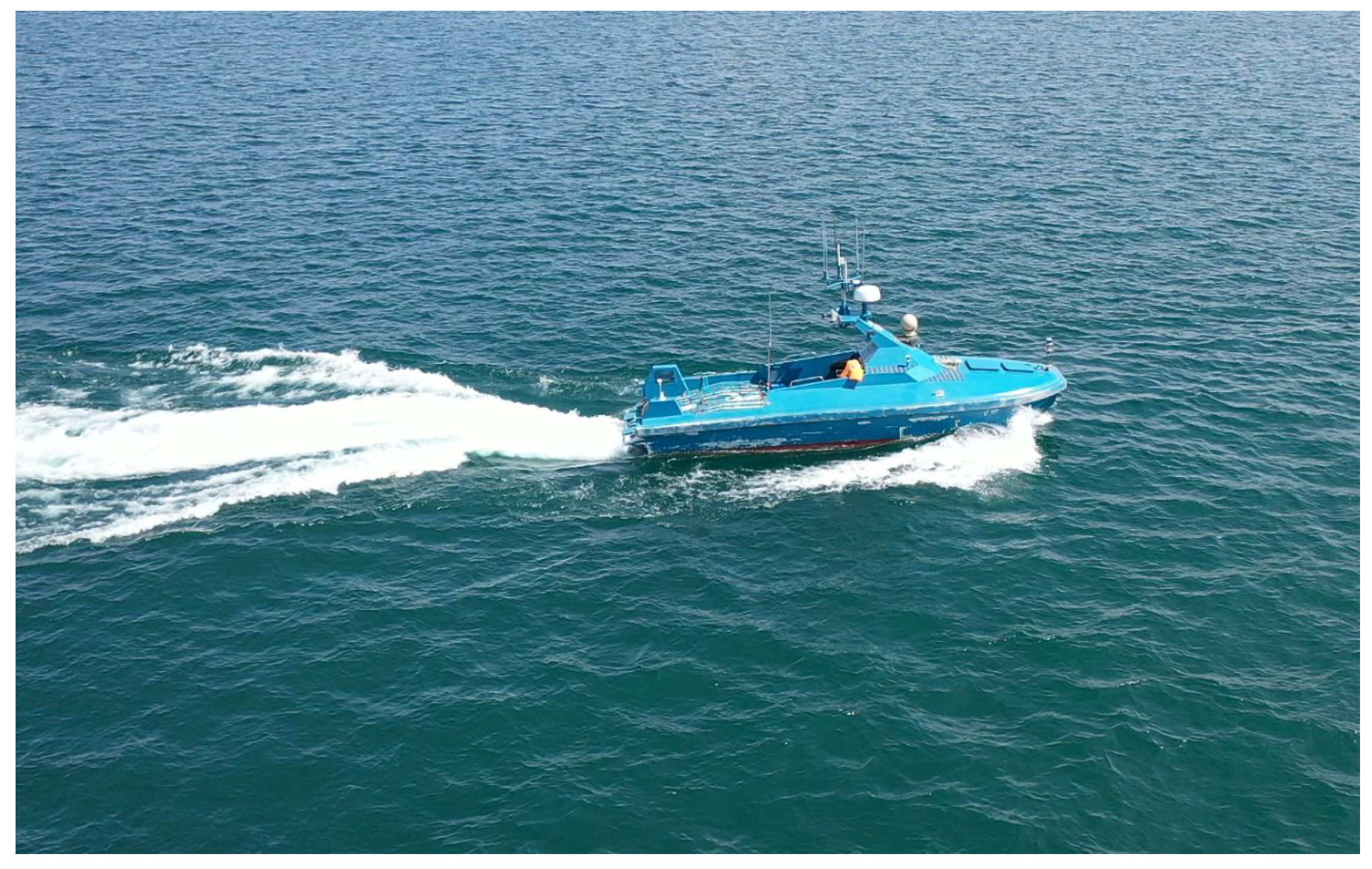
where $T_{port}$ and $T_{stbd}$ represent the thrust generated by the port and starboard thrusters, respectively, which can be derived from the thruster speeds. $\delta$ is the steering command angle of the full-scaled USV-900 (China Ship Scientific Research Center, Wuxi, China), features a dual-waterjet propulsion, offering enhanced maneuverability and stability for autonomous operations.

Despite a comprehensive understanding of the surface vehicle model, accurately estimating its hydrodynamic parameters remains a formidable challenge. These parameters, known as hydrodynamic coefficients, can be determined through either computational fluid dynamics (CFD) simulations or experiments [26]. Subsequently, the derived motion equation will serve as the foundation for training an online RL algorithm or for constructing a model-based controller, such as NMPC.

The USV-900, depicted in Figure 1, is a 12 m fiberglass unmanned surface vehicle designed and developed by the China Ship Scientific Research Center. The mass properties are presented in

Table 1. Model parameters.

Description	Symbol	Value
Length overall	$L_a$	12 m
Beam overall	$B_a$	3 m
Mass	m	7600 kg
Longitudinal center of gravity	$x_G$	0.23 m
Moment of inertia	$I_z$	51,193.3 kg ${\mathrm{m}}^2$

, and the hydrodynamic coefficients are shown in

Table 2. Non-dimensional hydrodynamic coefficients.

Coefficient	Value	Coefficient	Value
$X_{\dot{u}}^{\prime }$	−1.8 × 10−3	$Y_{\dot{v}}^{\prime }$	−3.66 × 10−2
$N_{\dot{v}}^{\prime }$	9.54 × 10−4	$N_{\dot{r}}^{\prime }$	−2.4 × 10−3
$X_{u\left|u\right|}^{\prime }$	−4.3 × 10−3	$Y_v^{\prime }$	−4.8 × 10−3
$Y_r^{\prime }$	−4.8 × 10−3	$N_v^{\prime }$	9.54 × 10−4
$N_r^{\prime }$	−2.4 × 10−3	/	/

.

2.2. Guidance Law for Path Following

We use the line-of-sight (LOS) based guidance method [25] to calculate during runtime the desired course angle. We first define a new desired vehicle point ${\mathbf{p}}_{los}(x_d,y_d)$. This point is positioned at a look-ahead distance $d>0$ from the vehicle’s direct projection onto the desired path. Here, the error vector between the desired position ${\mathbf{p}}_{los}$ and the current USV position $\mathbf{p}(x,y)$ is given by

$$\mathbf{e}={\mathbf{R}}_p^T\left({\alpha }_k\right)(\mathbf{p}-{\mathbf{p}}_{los})$$

(7)

$${\mathbf{R}}_p^T\left({\alpha }_k\right)=\left[\begin{array}{cc}cos{\alpha }_k& -sin{\alpha }_k\\ sin{\alpha }_k& cos{\alpha }_k\end{array}\right]$$

(8)

Equation (8) represents the rotation matrix between the NED frame and the path-parallel frame. The error vector $\mathbf{e}={[x_e,y_e]}^T$ consists of the along-track error $x_e$ and the cross-track error $y_e$. The cross-track error is the key control objective of the guidance law, which aims to drive this error to zero. It is defined as follows:

$$y_e=-\left[x\left(t\right)-x_k\right]sin{\alpha }_k+\left[y\left(t\right)-y_k\right]cos{\alpha }_k$$

(9)

The path-tangential angle, denoted as ${\alpha }_k$, signifies the intended heading along the specified path. Furthermore, the desired heading angle, ${\psi }_d$, which is given by $arctan(-y_e/d)$, indicates the relative heading angle intended to direct the vehicle’s heading towards the point ${\mathbf{p}}_{los}(x_{los},y_{los})$.

2.3. Markov Decision Process

In a MDP, defined by the tuple ($S,A,p,r$), both the state space S and action space A are continuous. The state transition probability p represents the likelihood of reaching the next state ${\mathbf{s}}_{t+1}\in S$ given the current state ${\mathbf{s}}_t\in S$ and action ${\mathbf{a}}_t\in A$. The environment provides a reward $r:S\times A\to \mathbb{R}$ for each state transition, which is used to train the stochastic policy $\pi \left({\mathbf{a}}_t\right|{\mathbf{s}}_t)$. The observation and action are defined as $\mathbf{s}=\left(e_{\psi },\dot{\psi },\delta \right)$ for path-following task. The reward function r is defined as

$$r(\mathbf{s},\mathbf{a})=-0.1e_{\psi }^2-{\dot{\psi }}^2-{\delta }^2$$

(10)

where $e_{\psi }={\psi }_d-\psi$ is heading angle error. The USV-900 steers by adjusting the nozzle angle $\delta$ during path-following. $\dot{\psi }$ is the yaw rate, and ${\psi }_d$ is the desired heading angle.

2.4. SAC-N Steering Controller

The SAC algorithm integrates three fundamental components: an actor–critic architecture with distinct policy and value function networks, an off-policy formulation to enhance data efficiency by reusing previously collected samples, and entropy maximization to promote stability and exploratory behavior. By increasing the number of Q-ensemble from 2 to N, SAC-N outperforms various offline RL algorithms by a large margin [24].

The primary goal of SAC-N is to maximize both the actor’s entropy and the expected reward. This dual objective ensures efficient learning while enhancing the system’s robustness. Entropy maximization promotes exploration by encouraging the actor to avoid deterministic decisions, thus improving stability and adaptability, which are particularly beneficial for uncertain environments like USV operations.

When applied to USVs, SAC-N offers substantial advantages in terms of training stability and control robustness. The constrained optimization problem can be reformulated as a dual problem, as shown in Equation (11), which seeks to balance reward maximization with entropy, allowing for improved exploration strategies in challenging maritime environments.

$$\underset{{\mathbf{a}}_t\ge 0}{min}\underset{{\pi }_t}{max}\mathbb{E}\left[r({\mathbf{s}}_t,{\mathbf{a}}_t)-{\alpha }_{t}log\pi \left({\mathbf{a}}_t\right|{\mathbf{s}}_t)\right]-{\alpha }_{t}H$$

(11)

where ${\alpha }_t$ is the dual variable. Furthermore, it can be rewritten as a optimization problem with regard to $\alpha$.

$$J\left(\alpha \right)={\mathbb{E}}_{a_t\sim {\pi }_t}\left[-\alpha log{\pi }_t\left({\mathbf{a}}_t\right|{\mathbf{s}}_t)-\alpha H\right]$$

(12)

The dual variable ${\alpha }_k$ and the entropy term H play critical roles in shaping the behavior of the SAC-N algorithm, facilitating a balanced approach to learning that emphasizes both reward accumulation and exploration. This balance is particularly advantageous when applied to USVs, where adaptive decision-making is vital for successful navigation and operation in dynamic environments.

In the policy evaluation step of soft policy iteration, we wish to compute the value of a policy $\pi$ according to the maximum entropy objective. For a fixed policy, the soft Q-value can be computed iteratively, starting from any function $Q:S\times A\to \mathbb{R}$ and repeatedly applying a modified Bellman backup operator given by

$$Q({\mathbf{s}}_t,{\mathbf{a}}_t)=r({\mathbf{s}}_t,{\mathbf{a}}_t)+\gamma {\mathbb{E}}_{{\mathbf{s}}_{t+1}\sim p}\left[V\left({\mathbf{s}}_{t+1}\right)\right]$$

(13)

where

$$V\left({\mathbf{s}}_t\right)={\mathbb{E}}_{{\mathbf{a}}_t\sim \pi }\left[\underset{j=1,...,N}{min}{Q}_{{\theta }_j}({\mathbf{s}}_t,{\mathbf{a}}_t)-\alpha log\pi \left({\mathbf{a}}_t\right|{\mathbf{s}}_t)\right]$$

(14)

Here, we use the minimum value of N parallel Q-networks to enforce their Q-value estimates to be more pessimistic.

The soft value function is trained to minimize the squared residual error,

$$J_V\left(\psi \right)={\mathbb{E}}_{{\mathbf{s}}_t\sim D}\left[{\displaystyle \frac{1}{2}}{\left(V_{\psi }\left({\mathbf{s}}_t\right)-{\mathbb{E}}_{{\mathbf{a}}_t\sim {\pi }_{\varphi }}\left[\underset{j=1,...,N}{min}{Q}_{{\theta }_j}({\mathbf{s}}_t,{\mathbf{a}}_t)-\alpha log{\pi }_{\varphi }\left({\mathbf{a}}_t\right|{\mathbf{s}}_t)\right]\right)}^2\right]$$

(15)

where D is the distribution of previously sampled states and actions, or a replay buffer.

The soft Q-function parameters can be trained to minimize the soft Bellman residual.

$$J_Q\left(\theta \right)={\mathbb{E}}_{({\mathbf{s}}_t,{\mathbf{a}}_t)\sim D}\left[{\displaystyle \frac{1}{2}}{\left(Q_{\theta }({\mathbf{s}}_t,{\mathbf{a}}_t)-\left(r({\mathbf{s}}_t,{\mathbf{a}}_t)+\gamma {\mathbb{E}}_{{\mathbf{s}}_{t+1}\sim p}\left[V_{\widehat{\psi }}\left({\mathbf{s}}_{t+1}\right)\right]\right)\right)}^2\right]$$

(16)

Finally, the policy parameters can be learned by directly minimizing the following expected Kullback–Leibler divergence Equation (17).

$$J_{\pi }\left(\varphi \right)={\mathbb{E}}_{\mathbf{s}\sim D}\left[D_{KL}\left({\pi }_{\varphi }\left(·|{\mathbf{s}}_t\parallel {\displaystyle \frac{exp\left(Q_{\theta }(\mathbf{s},·)\right)}{Z_{\theta }\left({\mathbf{s}}_t\right)}}\right)\right)\right]$$

(17)

A typical solution for minimizing $J_{\pi }$ is policy gradient methods, which is to use thee likelihood ratio gradient estimator without backpropagating the gradient through the policy and the target density networks. We reparameterize the policy using a neural network transformation,

$${\mathbf{a}}_t=f_{\varphi }({ϵ}_t;{\mathbf{s}}_t)$$

(18)

where ${ϵ}_t$ is an input noise vector, sampled from some fixed distribution, such as a spherical Gaussian. We rewrite the objective in Equation (18) as

$$J_{\pi }\left(\varphi \right)={\mathbb{E}}_{s_t\sim D,{ϵ}_t\sim N}\left[\alpha {log}_{{\pi }_{\varphi }}{\pi }_{\varphi }\left(f_{\varphi }({ϵ}_t;{\mathbf{s}}_t)\right|{\mathbf{s}}_t)-\left(\underset{j=1,...,N}{min}{Q}_{{\theta }_j}({\mathbf{s}}_t,{\mathbf{a}}_t)-V_{\psi }\left({\mathbf{s}}_t\right)\right)\right]$$

(19)

where ${\pi }_{\varphi }$ is defined implicitly in terms of $f_{\varphi }$. We can approximate the gradient of Equation (19) with

$${\widehat{\nabla }}_{\varphi }{J}_{\pi }\left(\varphi \right)={\nabla }_{\varphi }\alpha log\left({\pi }_{\varphi }\left({\mathbf{a}}_t|{\mathbf{s}}_t\right)\right)+\left({\nabla }_{{\mathbf{a}}_t}\alpha log\left({\pi }_{\varphi }\left({\mathbf{a}}_t\right|{\mathbf{s}}_t)\right)-{\nabla }_{{\mathbf{a}}_t}\underset{j=1,...,N}{min}Q({\mathbf{s}}_t,{\mathbf{a}}_t)\right){\nabla }_{\varphi }{f}_{\varphi }({ϵ}_t;{\mathbf{s}}_t)$$

(20)

where ${\mathbf{a}}_t$ is evaluated at $f_{\varphi }({ϵ}_t;{\mathbf{s}}_t)$.

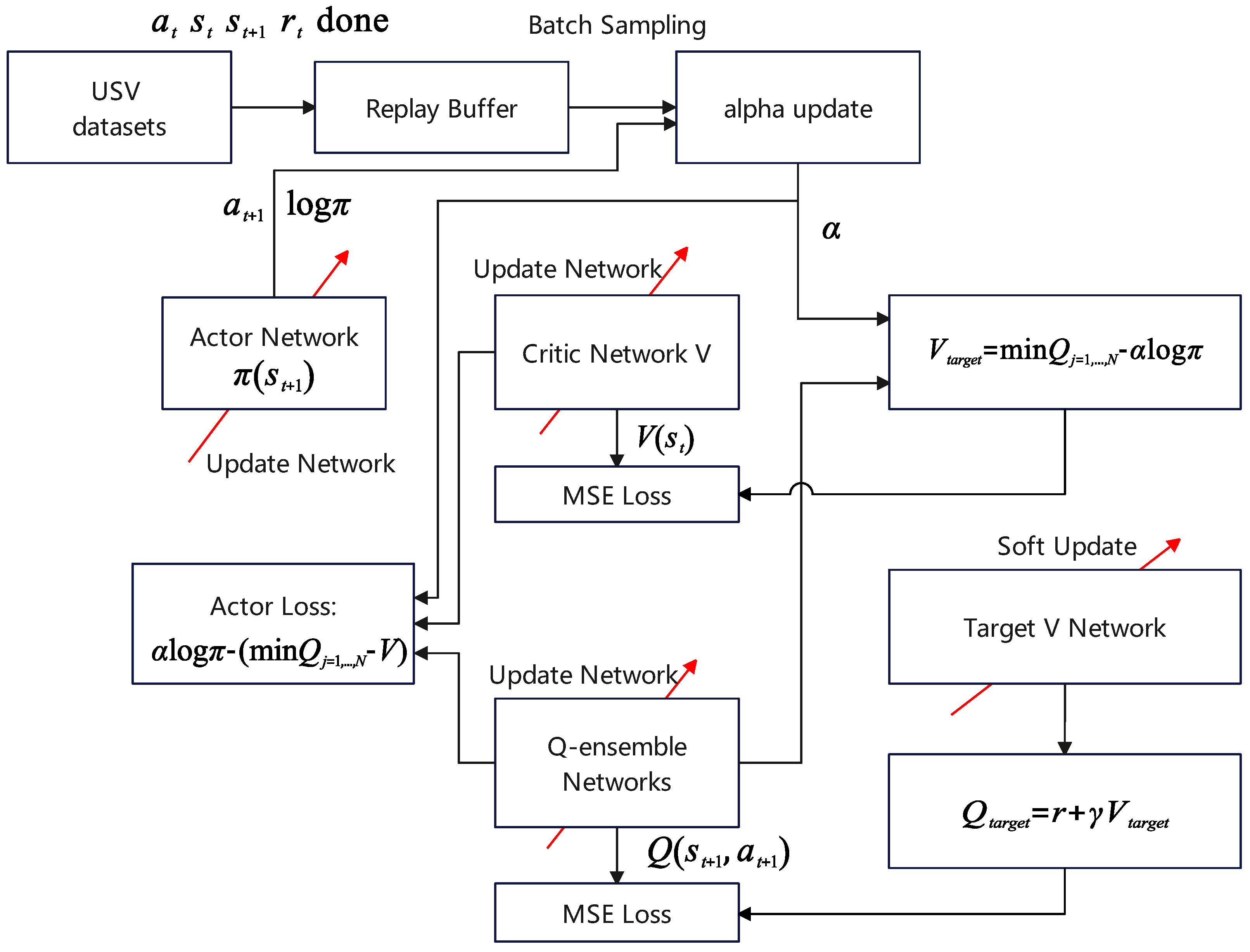
In Figure 2, we demonstrate the application of SAC-N for learning steering control directly from offline datasets. We utilize real-world trial datasets gathered from the USV-900, an unmanned surface vehicle propelled by waterjet systems. The action space encompasses steering commands, which are translated into the desired waterjet nozzle angle and precisely tracked via a PID controller. The observations encompass the desired heading angle, actual heading angle, angular velocity, and the current state of the waterjet nozzle angle. The reward function, specified in Equation (10), imposes penalties for large tracking errors, excessive angular velocities, and large nozzle angles.

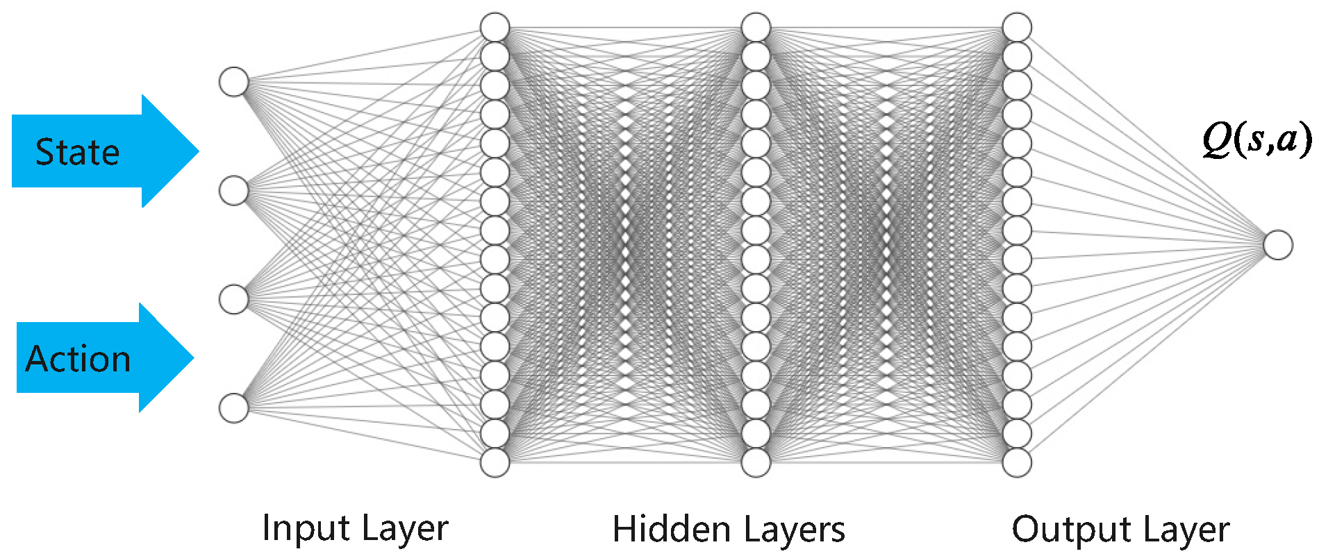
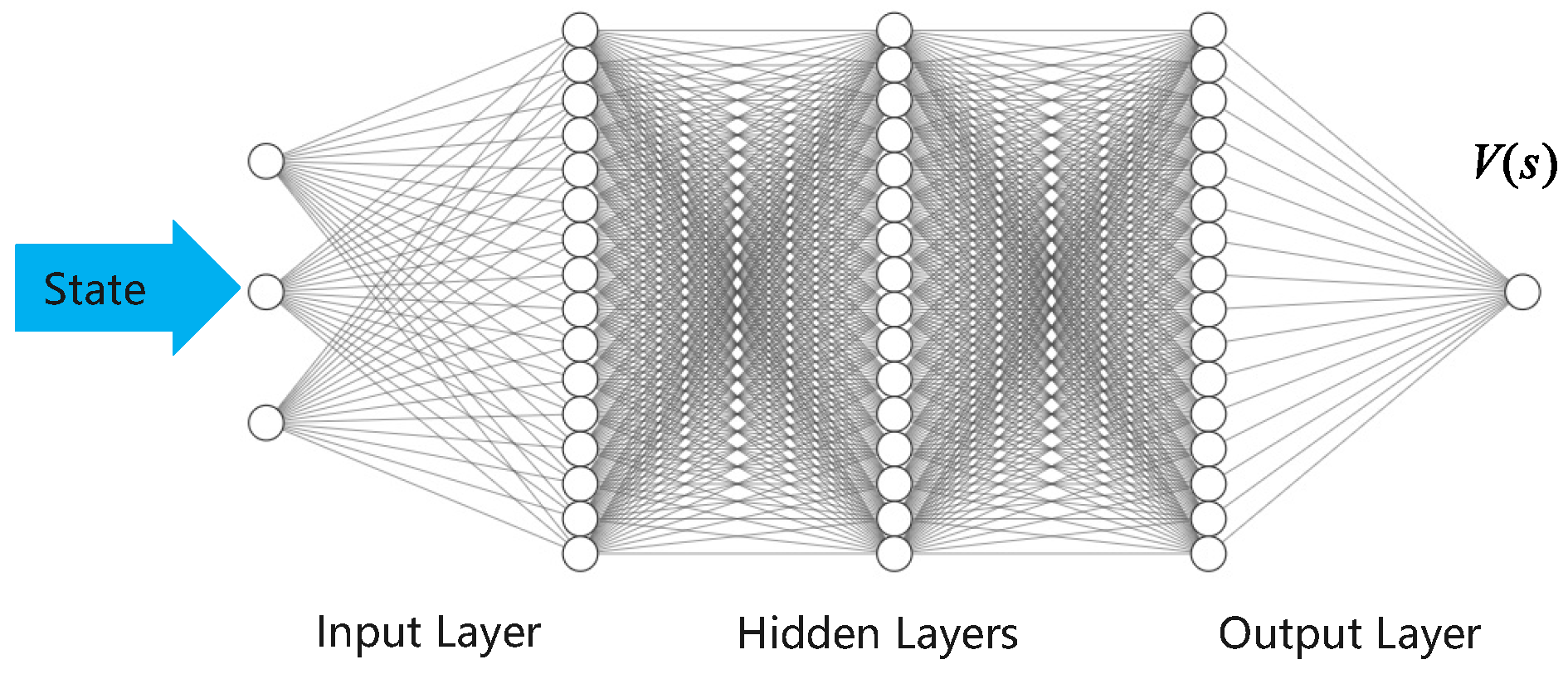
Our policy is represented by a feed-forward neural network consisting of two hidden layers, each with 64 neurons, as illustrated in Figure 3. The critic Q-function and value functions, illustrated in Figure 4 and Figure 5, are implemented using neural networks with two hidden layers, each comprising 64 neurons.

2.5. Training

SAC-N utilizes offline datasets collected from the USV-900 trials for training. To obtain the state variables during the experiments, we employed on-board navigation sensors, including an inertial measurement unit (IMU) and the BeiDou satellite system (BDS), to capture high-precision positional data. An embedded computer was utilized to record device-related information, such as engine speed and waterjet nozzle angle. The collected data were stored in an SQLite database.

All training was conducted on an Intel Core i5-11400H CPU (Integrated Electronics Corporation, Fresno, CA, USA) running at 2.70 GHz. During training, the Adam optimizer was employed to update the parameters of both the actor and value networks. The hyperparameters used are outlined in

Table 3. The hyperparameters selected for training the SAC-N controller.

Hypeparameter	Value
actor learning rate	3 × 10−4
critic learning rate	3 × 10−4
alpha learning rate	3 × 10−4
optimizer	Adam
max action	1.0
datasets size	200,000
batch size	128
soft target update parameter	5 × 10−3
gamma	0.99
hidden dimension	64
activate function	ReLU
log standard range	[−5, 2]

.

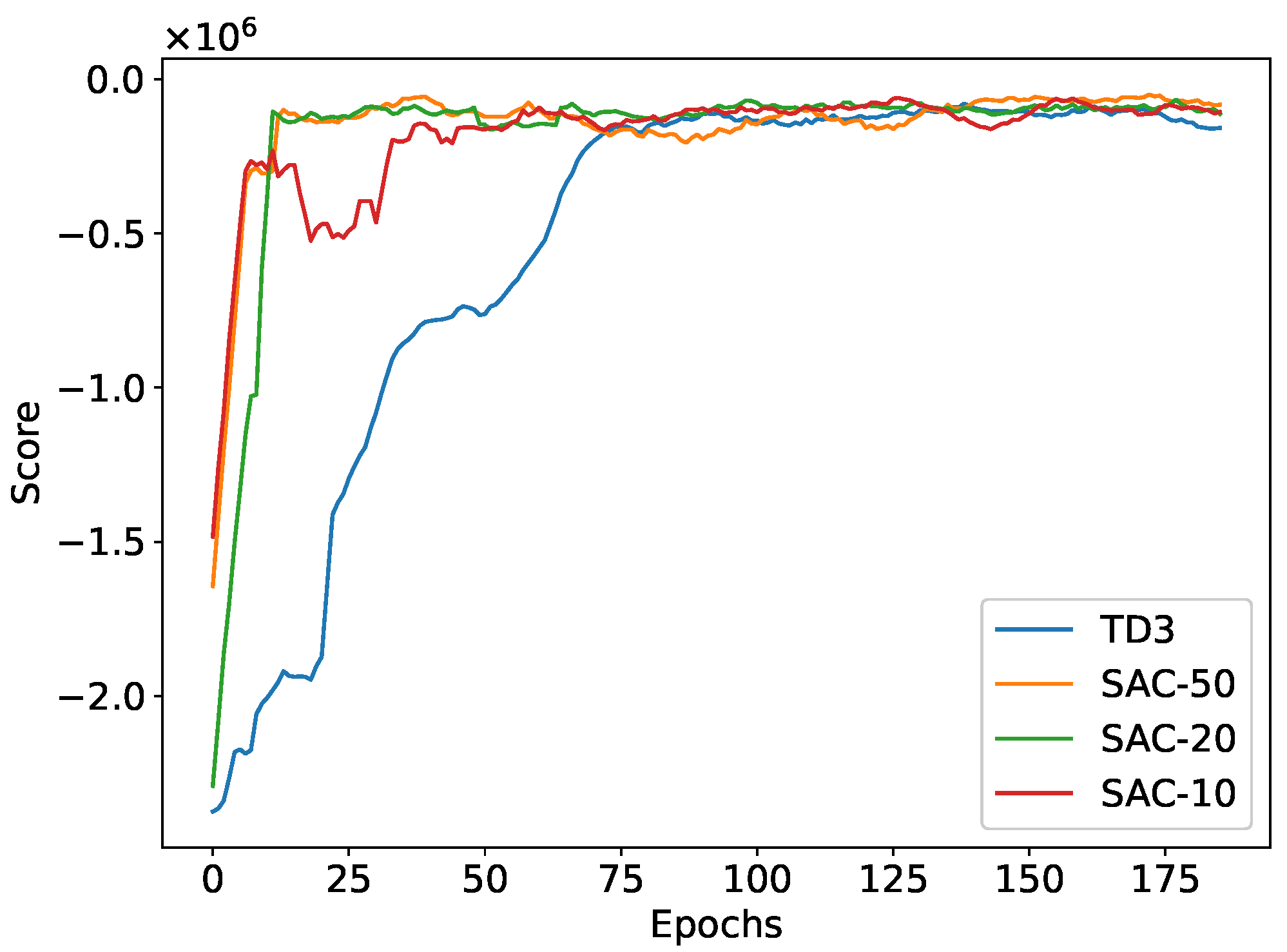
Figure 6 illustrates the average returns from evaluation rollouts during the training process for both TD3 and SAC-N. In SAC-N, the ensemble size N was incrementally increased to values of 10, 20, and 50, allowing the algorithm to achieve comparable performance to TD3 in a shorter training duration. SAC-N demonstrated higher data efficiency and stability, reaching optimal performance more rapidly than TD3. The final average return of SAC-N consistently improved with larger N values; notably, N = 50 achieved a higher average return than both N = 20 and N = 10, and all SAC-N variants outperformed TD3. For the USV path-following simulations and tests, SAC-50 was employed as the steering controller.

The superior performance of SAC-N can be attributed to its clipped Q-learning approach, which selects the minimum Q-value from the ensemble to produce a conservative estimate. This pessimistic estimation strategy significantly enhances SAC’s stability and robustness by mitigating the risk of overestimation. Consequently, it boosts overall training efficiency and effectiveness in achieving optimal control.

3. Validation

To evaluate the performance of our proposed SAC-N steering controller, we conducted several USV simulations and free-running tests using the USV-900. For validation, we completed a comparative analysis against several established controllers.

3.1. Simulation Results

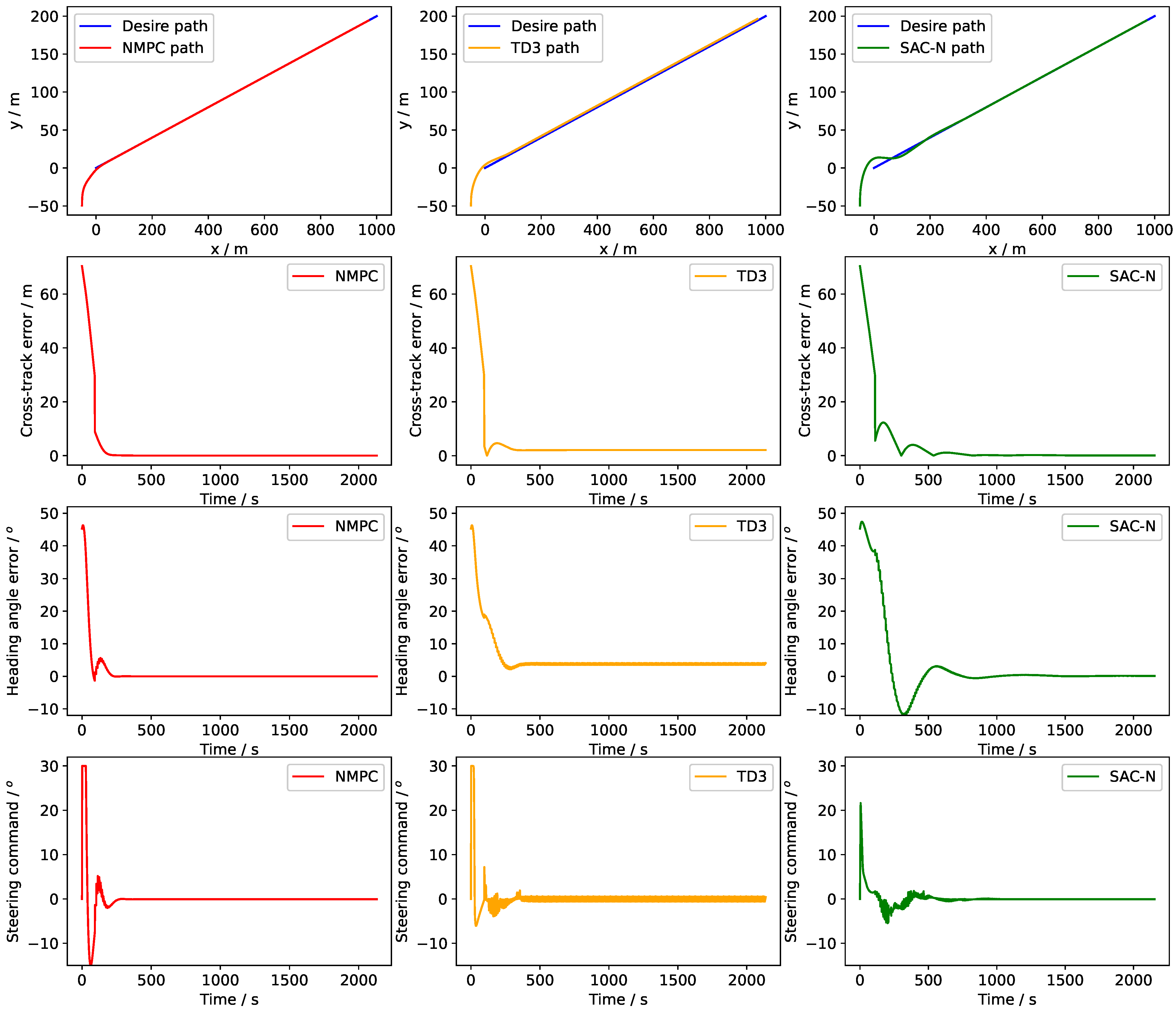
To evaluate the self-learning capability of the proposed method, we compared SAC-N with NMPC and TD3 in simulations. NMPC typically involves establishing complex multi-input multi-output (MIMO) discrete state-space equations for nonlinear dynamic models, and solving constrained quadratic programming problems in real-time to obtain a sequence of optimal control variables. Usually, the first element in this sequence is used for real-world control. It effectively guides the USV along a desired trajectory while taking into account nonlinear dynamics and environmental disturbances, such as currents and wind. TD3, an enhancement of DDPG, learns an optimal policy that directly outputs continuous steering commands. In the path-following simulation, the target path was defined as a straight line with a starting point at (0, 0) and an endpoint at (1000, 200).

The speed of the USV is set to 10 knots. The initial position of the USV is (−50,−50), with an initial heading angle of zero. The simulation time step was set to 0.1 s. In terms of performance indicators, we use the mean absolute error (MAE) of the heading angle, cross-track MAE, and steering commands to evaluate the performance.

Figure 7 compares the path-following performance of NMPC, TD3, and SAC-N. Compared to TD3, SAC-N shows better performance in terms of steady-state error, with the error approaching zero after stable line tracking. In contrast, TD3 exhibits persistent steady-state error and oscillations in the steering commands. Compared to NMPC, SAC-N generates smaller steering commands, which helps reduce the axial force reduction caused by steering. According to

Table 4. Comparison of simulation results using various controllers.

Controller	Heading Angle MAE (°)	Cross-Track MAE (m)	Mean Absolute Steering Command (°)
NMPC	2.4	1.1	0.9
TD3	4.4	5.4	0.8
SAC-N	3.7	4.4	0.5

, SAC-N and NMPC have smaller cross-track errors than TD3. Higher steering commands lead to increased energy consumption, and the nozzle angle can influence the axial force and surge velocity.

3.2. Test Results

To validate the path-following performance of the SAC-N controller, we conducted a comparison with PID, NMPC, and TD3 controllers in path-following tests on the USV-900. PID is a linear controller that operates without the need for a model, with tuning parameters set based on an engineer’s experience. In contrast, NMPC relies on the state-space equations of the USV-900. TD3, meanwhile, trains through online interaction with a simulator that employs the motion equations of the USV-900. SAC-N learns a steering policy by training on predefined datasets (https://huggingface.co/datasets/babaka/usv_tracking_sac_pretrain_dataset/tree/main (accessed on 25 November 2024)). These data were recorded during the manual operation of the USV and were subsequently organized into a dataset. The dataset comprises 200K transitions, each represented as $\left({\mathbf{s}}_t,{\mathbf{a}}_t,{\mathbf{r}}_t,{\mathbf{s}}_{t+1},done\right)$.

During the path-following tests, the USV was operated at a constant speed of around 10 knots to maintain consistent conditions throughout the trials. The experiments took place in a marine area with a sea state of level 3, ranging in height from 0.5 to 1.25 m, where conditions were influenced by random ocean currents, offering a realistic evaluation of the controller’s robustness and adaptability in dynamic environments.

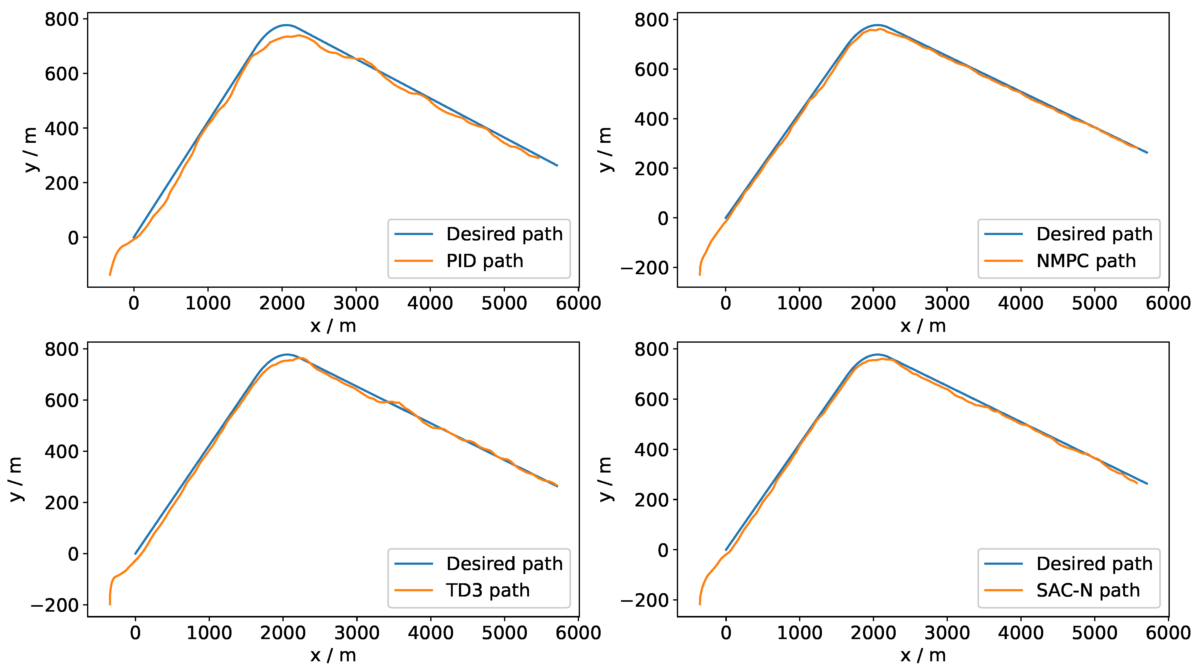
After adjusting the parameters and training the policy networks, each steering controller was implemented in Python 3.10.14 and Pytorch 2.3.0 and deployed onto an embedded computer on the USV-900. The reference path consists of two straight segments, with a circular arc of radius 300 m connecting them at the corner, tangent to both straight lines. The starting point of the reference path is (0, 0), and the endpoint is (5707.46, 263.31). The endpoints of the arc are (1637.26, 692.19) and (2198.89, 767.70). The desired path consists of 52 points in total. The USV employs LOS guidance to track discrete line segments.

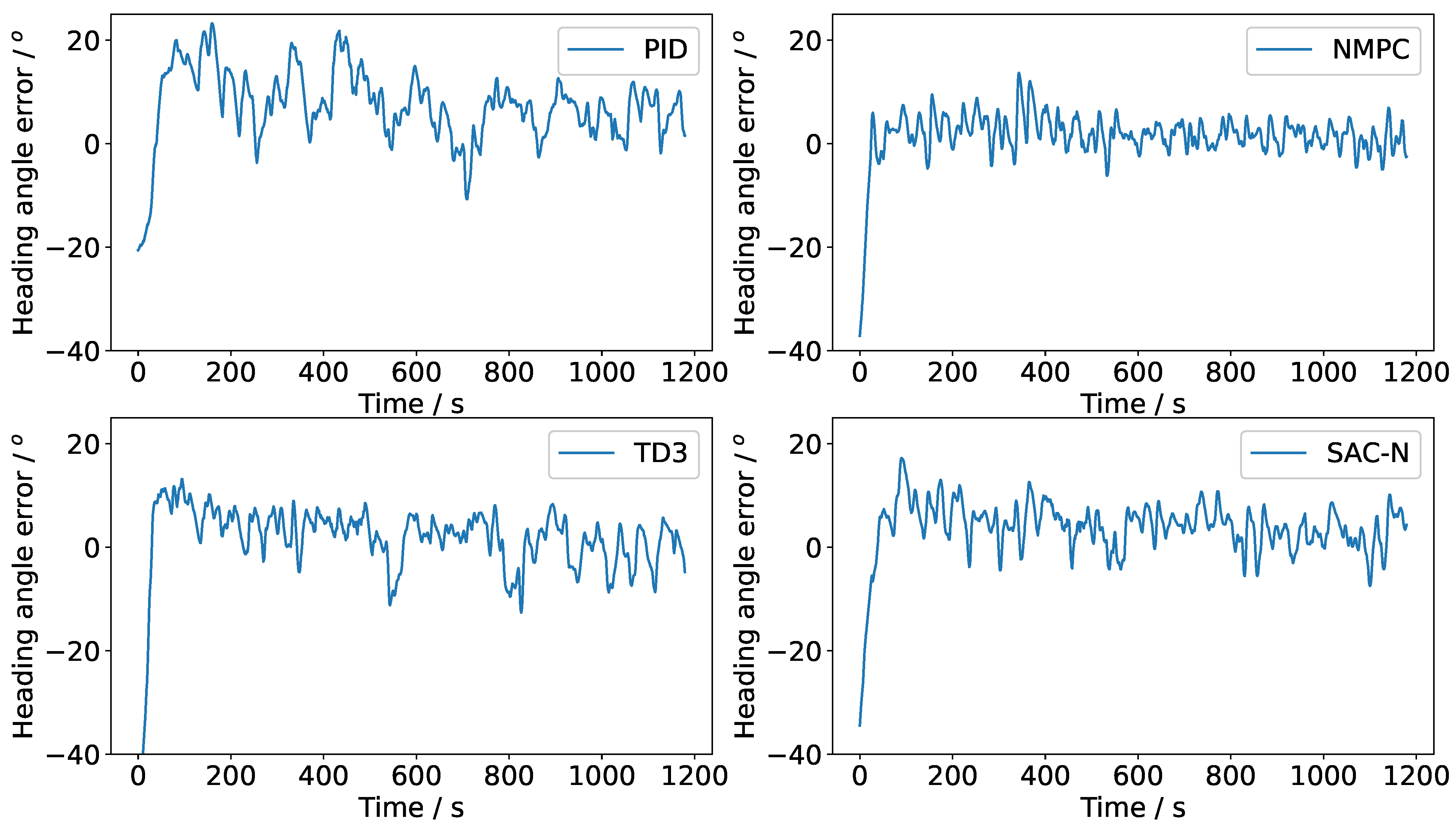
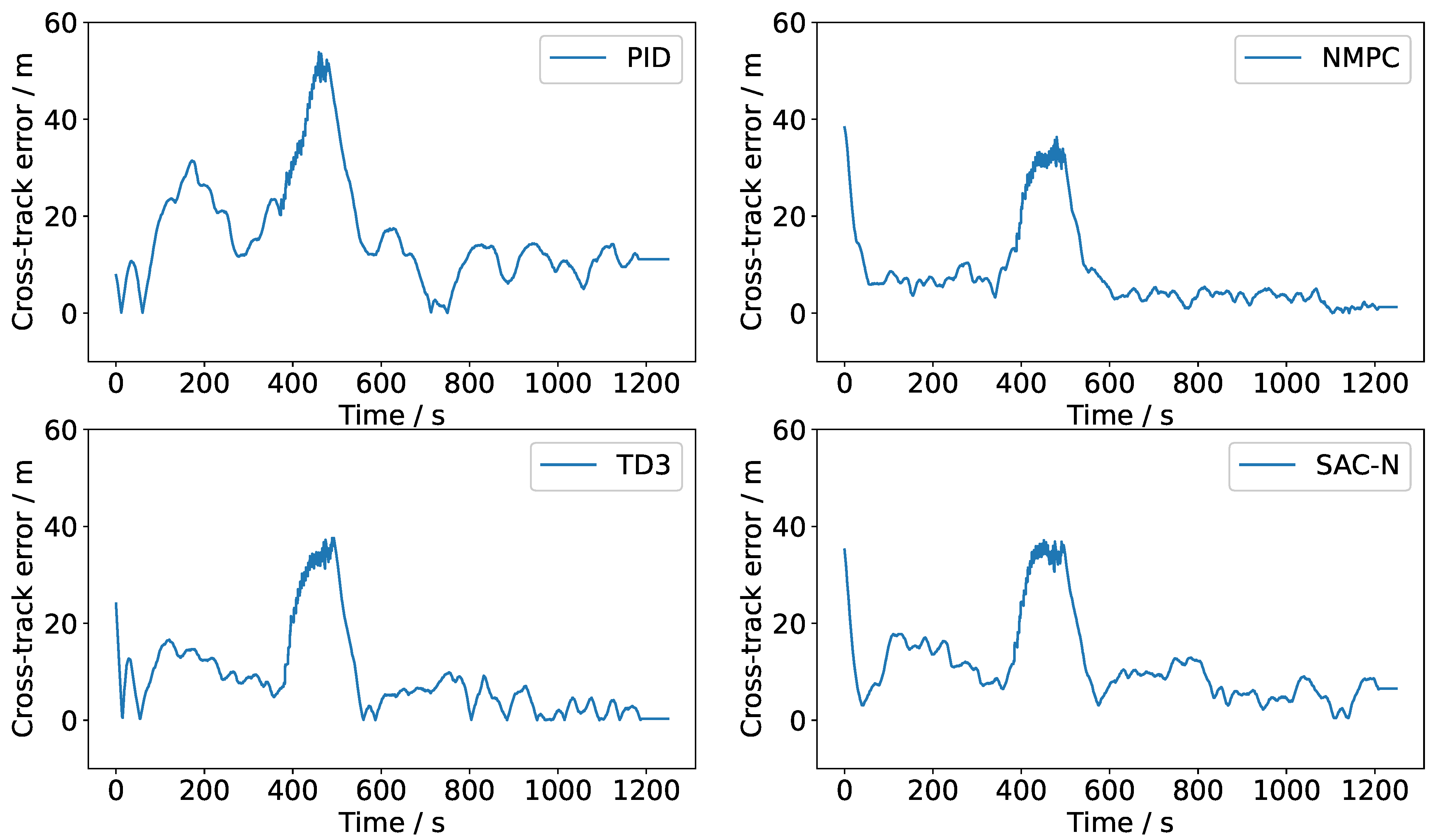
Figure 8 compares the path-following trajectories of various controllers, namely PID, NMPC, TD3, and SAC-N. The trajectory of the USV and the desired path are transformed from WGS84 coordinates to universal transverse mercator (UTM) coordinates, with the first point of the desired path set as the origin. Figure 9 and Figure 10 illustrate the changes over time in the heading angle error and cross-track error, respectively, during the path-following tests.

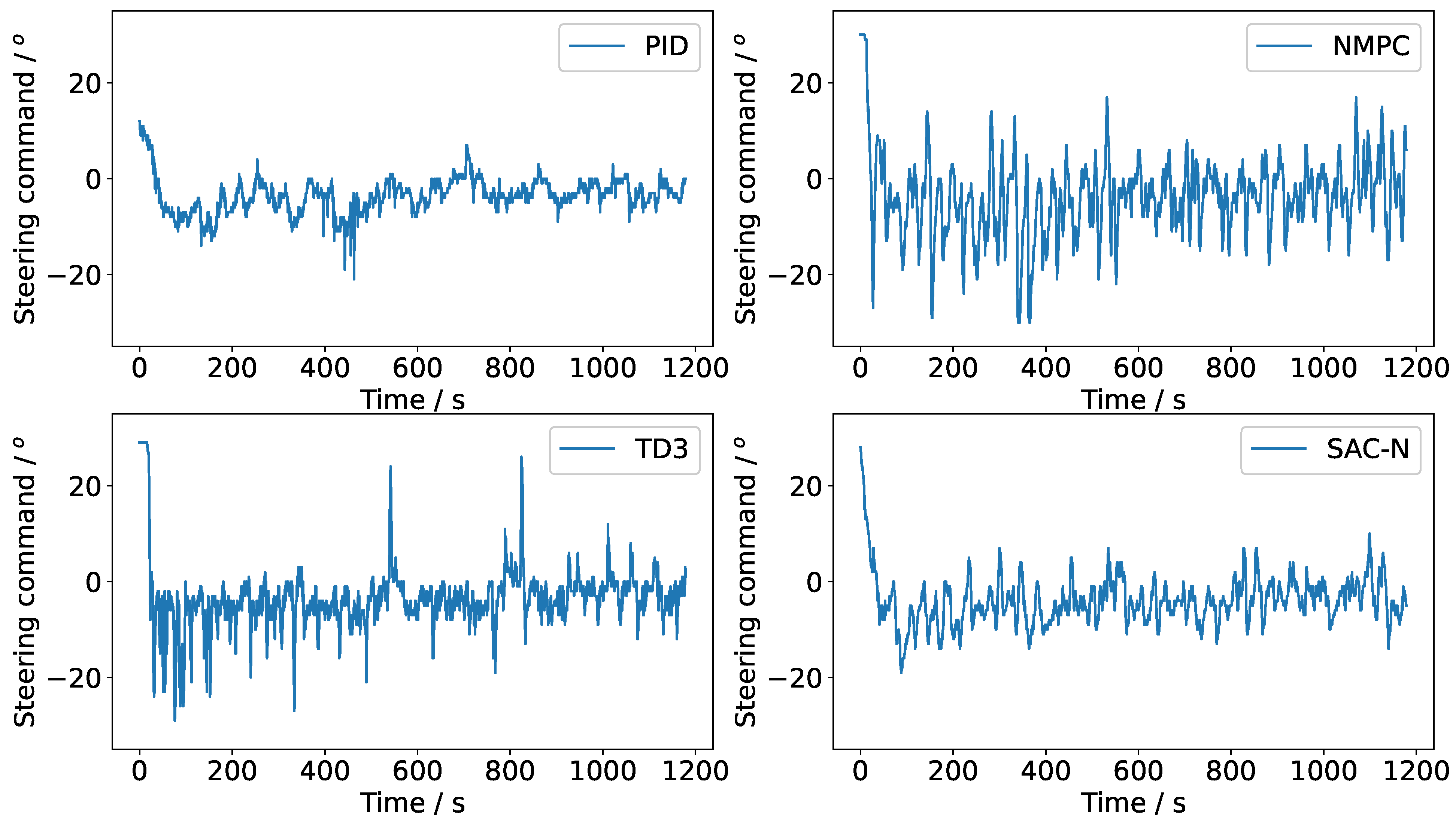
Figure 11 illustrates the steering command curves for various controllers. The experimental results indicate that NMPC, TD3, and SAC-N performed comparably. However, all controllers struggled to consistently converge towards zero error due to random disturbances from wind and wave loads. To mitigate these disturbances, the steering command was adjusted promptly. While NMPC is the optimal controller, the DRL-based controllers (TD3 and SAC-N) achieved a more favorable balance between precise tracking and steering maneuverability, demonstrating high tracking performance with minimal steering commands. Notably, the steering command angle of SAC-N was significantly smaller than that of NMPC, which typically results in reduced axial thrust loss. This highlights SAC-N’s advantage in attaining high performance with minimal steering effort.

Table 5. Performance of different controllers in path-following test with real-life USV. “Consumption time” is the average time needed for generating a single-step steering command.

Controller	Heading Angle MAE (°)	Cross-Track MAE (m)	Mean Absolute Steering Command (°)	Consume Time (ms)
PID	8.64	16.3	4.14	0.064
NMPC	3.18	7.9	6.67	16.29
TD3	5.18	8.6	5.42	1.86
SAC-N	5.31	11.3	5.33	2.62

provides a detailed comparison of the performance of various controllers. The cross-track error is defined as the perpendicular distance from the current position of the USV to the nearest point on the discrete tracking line segment. PID exhibits the fastest real-time performance due to its simple calculation process; however, its tracking accuracy is the lowest. In contrast, while NMPC achieves the highest tracking accuracy in terms of heading angle and cross-track error, it demands a significant amount of CPU time and generates large, high-frequency steering commands. Although NMPC demonstrates strong robustness, solving consecutive multi-step quadratic programming problems iteratively can hinder its real-time performance.

When comparing TD3 and SAC-N, TD3 performs better in terms of mean absolute error (MAE) indicators. However, SAC-N has the advantage of requiring only offline datasets, which eliminates the need for interactions with simulators or experimental setups, leading to significant savings in training costs. In contrast, TD3 cannot learn from fixed datasets and relies heavily on online interactions. As a result, online training on a real-world unmanned surface vehicle (USV) is slow, with each training step requiring more time due to actuator delays and the vehicle’s relatively low speed. Specifically, TD3 requires online training for 200,000 frames, resulting in a training time of 7.5 h. In contrast, SAC-N can be trained offline in just 1.2 h.

SAC-N utilizes the minimum Q-value from N Q-networks, which reduces the risk of overestimation. This allows it to achieve performance and stability comparable to TD3 when trained on offline datasets. This highlights the advantages of using offline model-free DRL controllers.

4. Conclusions

Classical online reinforcement learning methods for path-following control tasks require interaction with a real-world USV. On the one hand, the USV’s state changes occur over a relatively long period, leading to slow online training. On the other hand, online training may result in incorrect actions that could potentially damage the USV. To address this issue, this paper introduces the SAC-N steering controller. This offline, model-free deep reinforcement learning algorithm enables low-cost self-learning of control policies while ensuring robust control. The SAC-N steering controller was successfully trained using collected datasets and validated through simulations of the USV’s behavior along a straight path and in a real-world experiment. After training, the performance of SAC-N is comparable to TD3, but the training process is safer and faster, eliminating the need for online data. Therefore, when policy performance is similar, SAC-N offers superior efficiency.

We compared SAC-N with PID, NMPC, and TD3. The results demonstrate that our practical DRL algorithm, used to train a deep neural network policy, matches the performance of NMPC and TD3. Our experiments show that the SAC-N steering controller is robust and efficient for path-following tasks in underactuated USVs. In future work, we plan to extend its capabilities to collision avoidance and more complex tasks and to train offline RL algorithms using vision-based inputs.