Underwater Drag Reduction Failure of Superhydrophobic Surface Caused by Adhering Spherical Air Bubbles

Abstract

Underwater drag reduction using superhydrophobic surfaces is a promising method due to its simplicity and low energy consumption. However, most attempts to obtain drag reduction using superhydrophobic surfaces have failed. Explanations such as air layer or air bubble vanishment and surface roughness are proposed in the existing works. In this work, the drag increase caused by spherical air bubbles adhering to the superhydrophobic surface is reported, and the drag increase mechanism is revealed by numerical simulation. In the water tunnel and towing tank experiment, we found that the experimental samples exhibited drag increase around a specific velocity, and the recorded optical images showed that the superhydrophobic surfaces were adhered by spherical air bubbles. Through numerical simulation, we found that the spherical air bubbles not only reduced the frictional drag but also introduced pressure drag. The drag increase was produced when the introduced pressure drag exceeded the reduced frictional drag. This work might be helpful for the drag reduction application of the superhydrophobic surface.

1. Introduction

Due to the viscosity of water, objects experience frictional drag when they travel underwater. Reducing frictional drag will save energy and improve traveling speed. Ways to reduce frictional drag can be divided into two classes. The first class reduces frictional drag based on the principle of boundary layer control. This class includes riblet surface [1,2], vibrating surface [3,4], and polymer additive [5,6]. The second class reduces frictional drag using lubricant. Both air [7,8] and oil [9,10] can be utilized as the lubricant. The application of superhydrophobic surface has been widely studied for its capacity of trapping air bubbles.

The superhydrophobic surface is characterized with a contact angle (CA) larger than 150° and a sliding angle less than 10°. The superhydrophobic surface, such as lotus leaf, is water-repellent, and water droplets can easily roll off from it. The mechanism of super hydrophobicity is that the micro/nanocavities on the superhydrophobic surface are occupied with air. The superhydrophobic surface mainly consists of materials with low surface energy and micro-/nano-surface texture. Two common methods, dip coating [11] and spray coating [12], are capable of preparing superhydrophobic coating on a surface with a large area and curvature. The dip–coating method is one type of subtle method that protects the original surface texture. Zhang et al. [13] prepared hydrophobic coating on the grooved hydrophilic surface by the dip–coating method and successfully turned the hydrophilic surface into a hydrophobic surface. The surface grooves were intactly protected. Hu et al. [14] prepared superhydrophobic coating on a micro-column patterned surface by the dip–coating process. The superhydrophobic coating was successfully obtained, and the micro-columns were protected. The spray-coating method is one kind of quick and simple method which can be applied to a wide range of substrates. In the work of Celik et al. [15], hydrophobic silica nanoparticles and wax were dispersed into chloroform, and then the mixed solution were sprayed onto the substrate and successfully turned the substrate into superhydrophobic. Zhang et al. [16] reported that the spray coating of octadecyltrichlorosilane can be applied to materials like plywood, filter paper, aluminum, cotton fabric, and plastic. Chen et al. [17] reported to have prepared superhydrophobic coating on the large-scale stainless steel (300 mm × 300 mm × 1.5 mm) by the spray-coating method. These two methods make it realizable for the application of underwater superhydrophobic drag reduction.

The reported drag reduction performance of the superhydrophobic surface are consistent in the experiments conducted in the rheometers or the Taylor–Couette apparatus. For example, Barbier et al. [18] conducted experiments in a rheometer and obtained the drag reduction rate of 3∼25% on all the examined hydrophobic surfaces. Chen et al. [19] conducted experiments in a rheometer and obtained the drag reduction rate of 3∼35% on the examined superhydrophobic surface. Saranadhi et al. [20] conducted experiments in a Taylor–Couette apparatus and reported to obtained the drag reduction rate over 75%. Rajappan and McKinley [5] conducted experiments in a Taylor–Couette apparatus and obtained the drag reduction rate of 5∼30% for the examined superhydrophobic surface. The potential explanation to this consistent drag reduction might be the strong viscous force. For experiments conducted in the rheometers or the Taylor–Couette apparatus, the water flow is driven by the shearing force between the rotor and the water. In this condition, the viscous force is stronger than the inertia force. The air bubbles are good at reducing frictional drag and thus produce consistent drag reduction.

However, the reported drag reduction performance of the superhydrophobic surface are inconsistent in the experiments conducted in wall-bounded turbulent flows. Aljallis et al. [21] reported drag increase caused by the loss of air bubbles. Bidkar et al. [7] and Gose et al. [22] reported drag increase caused by the surface roughness. Bidkar et al. [7] concluded that the surface roughness should be smaller than the thickness of the viscous sublayer. Ling et al. [23], Abu Rowin and Ghaemi [24,25] conducted experiments in wall bounded turbulent flow to investigate the influence of the superhydrophobic surface on the near wall flow field. Their results showed that the surface roughness intensified the turbulence and increased the frictional drag. Reholon and Ghaemi [26] reported the drag reduction failure caused by the air bubble dissolution.

In this work, the drag reduction failure caused by the spherical air bubbles is reported. In the experiments conducted to investigate the drag reduction effect of the superhydrophobic surface, we found that the spherical air bubbles arise automatically around a specific velocity and the drag dramatically increases at the mean time. We suspect that the drag increase is caused by the spherical air bubbles and the numerical simulation is applied to verify our suspicion and reveal the drag increase mechanism.

2. Materials and Methods

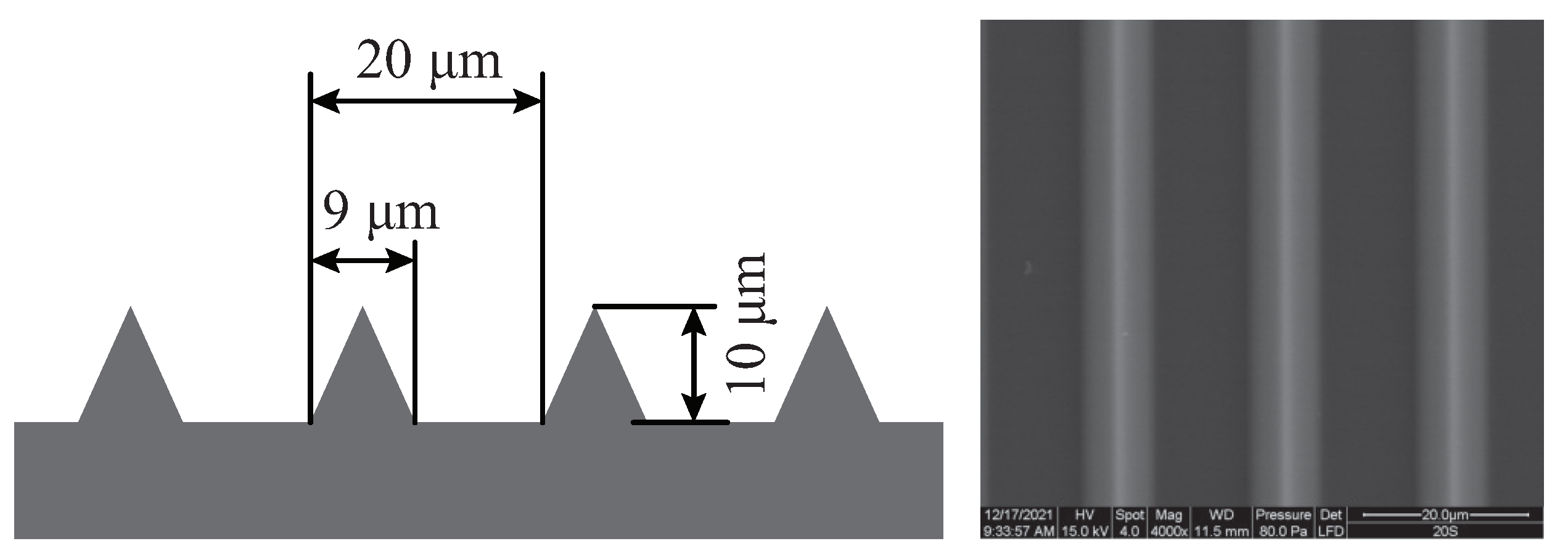
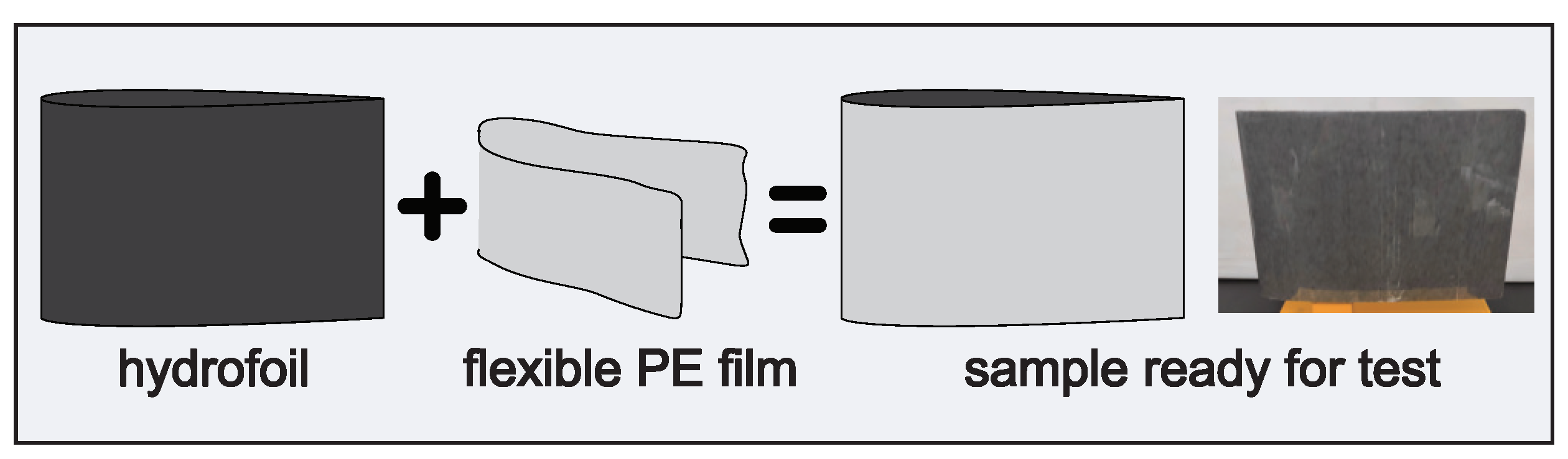
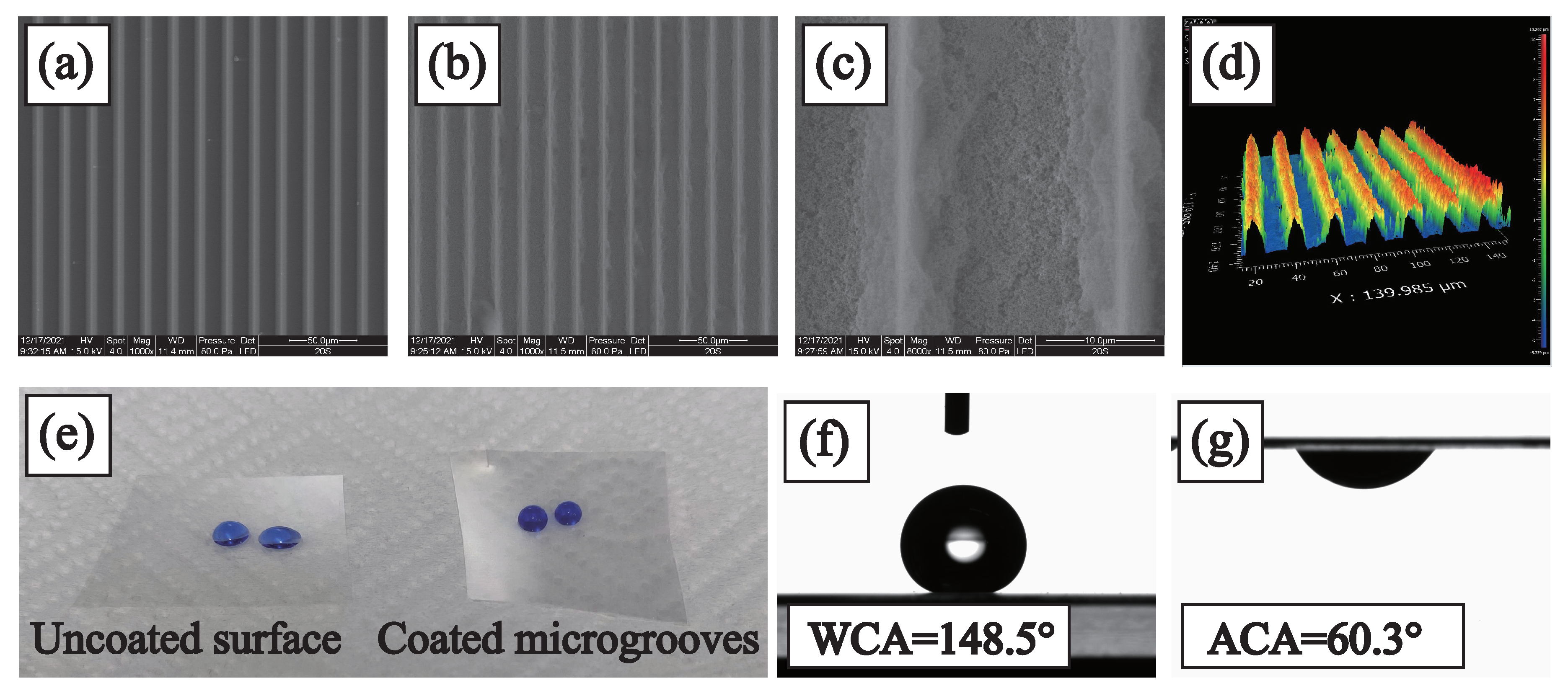
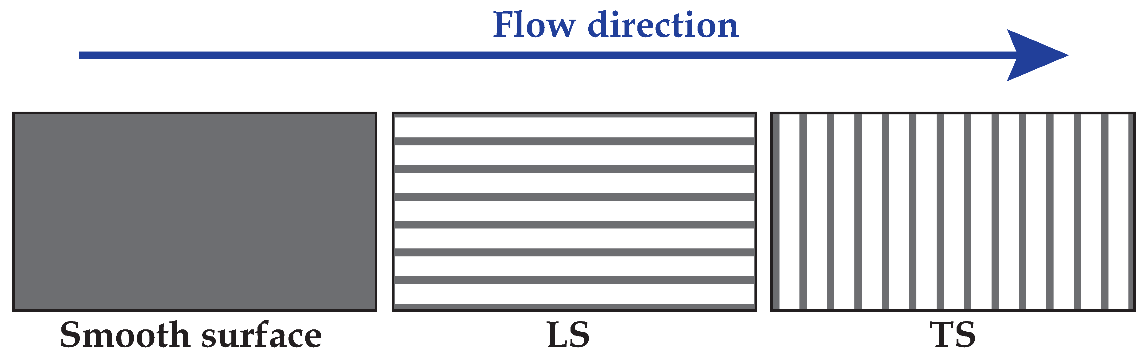
2.1. Sample Preparation

It is reported that superhydrophobic microgrooves exhibit good drag reduction performance [8,27]. Thus, the superhydrophobic surface used in this work is microgrooves coated with hydrophobic nanoparticles. The microgrooves are printed on flexible polyethylene (PE) film by ultraviolet light polymerization. The flexible PE film is about 100 µm thick, and more details about the PE film can be obtained from Kangdexin Composite Material Group, China. The used microgroove (Figure 1) is 10 µm in depth and 20 µm in width. The cross section of the rib is triangle and is 9 µm in width.

The original PE film is hydrophilic, which is unable to trap air. In order to modify the wettability of the PE film and avoid blocking the microgrooves, a dip-coating method was used (Figure 2). The cleaned PE film was firstly immersed into the ethanol solution of Evo-stick for 15 min. The Evo-stick (bought from www.taobao.com (accessed on 7 January 2021)) served as binder, and its mass fraction in the ethanol solution was 2%. After the immersion was finished, the PE film was dried in an oven at 60 °C for 15 min. Then, it was immersed into the ethanol solution of hydrophobic silica nanoparticles (HSNPs) for 15 min. The HSNP (Aerosil A972, bought from www.taobao.com) served as the hydrophobic agent, and its mass fraction in the ethanol solution was 3%. Finally, the PE film was dried in the oven at 60 °C for 15 min, and the superhydrophobic PE film was obtained.

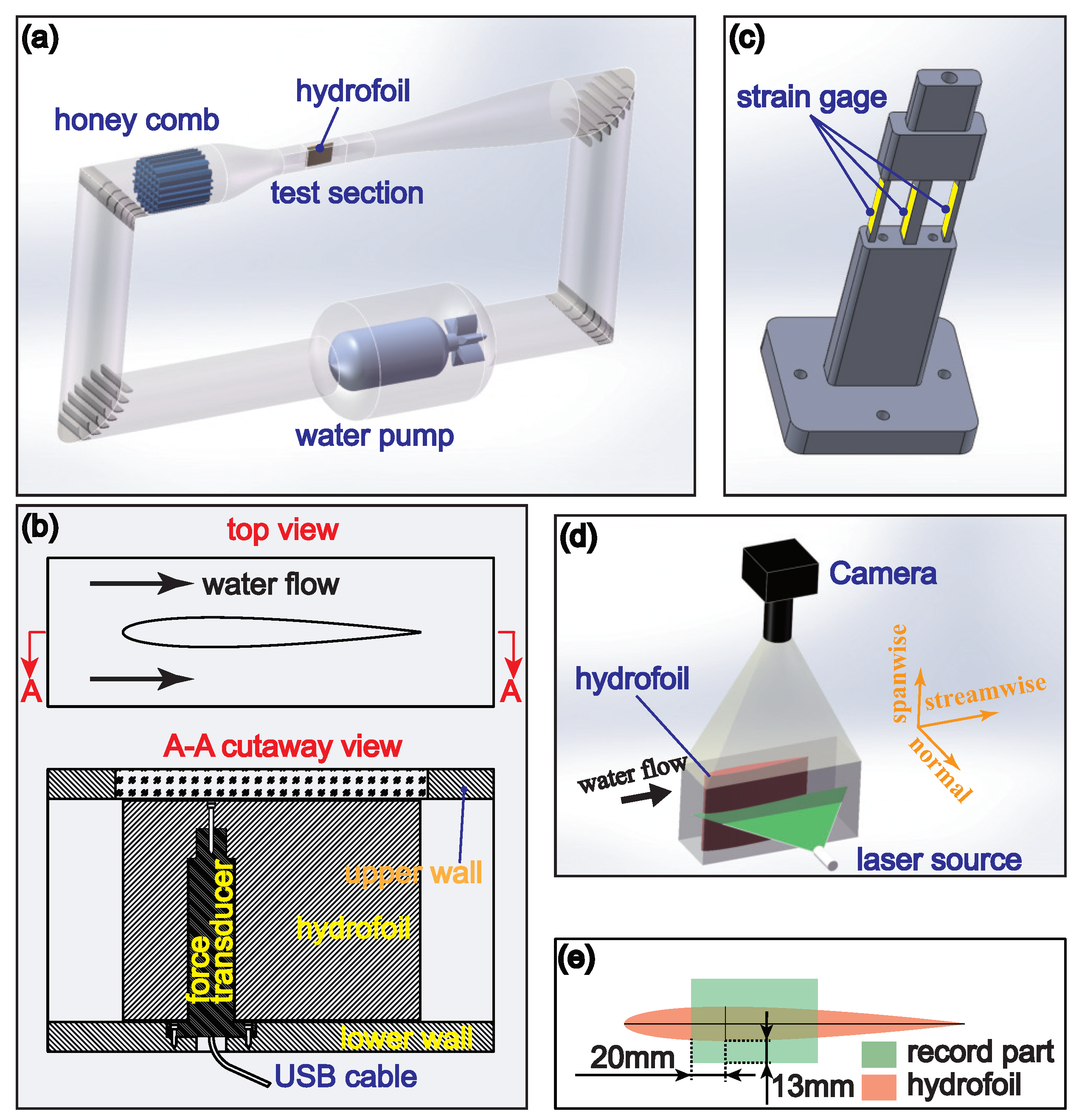
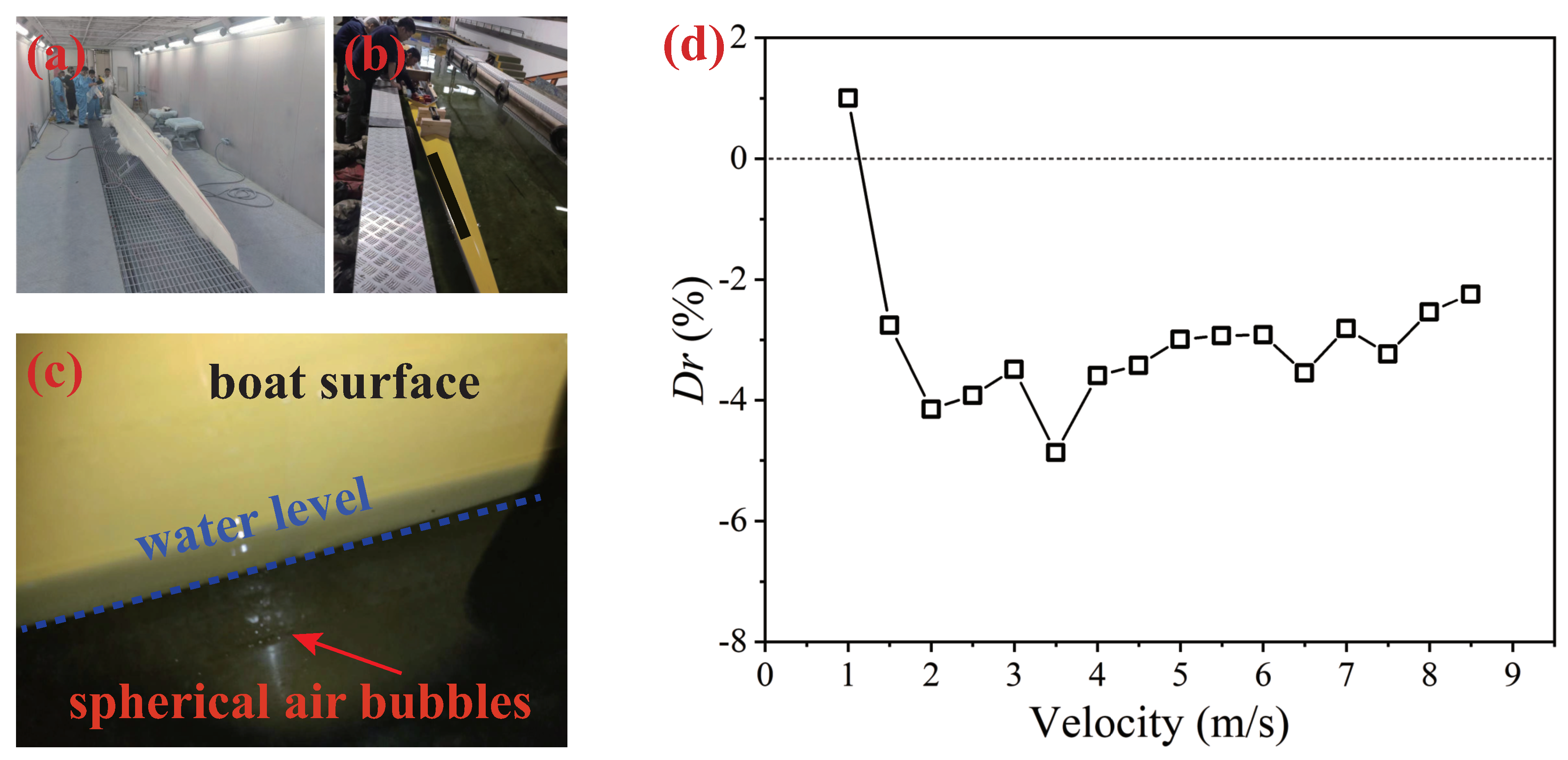
2.2. Hydrodynamic Experiment

The hydrodynamic experiment was conducted in a water tunnel (Figure 3a). The width, height, and length of the test section (Figure 3b) are 100 mm, 150 mm, and 300 mm, respectively. Within the test section, a force transducer (Figure 3c) was used to record the force. The force transducer is bought from the Aerodynamics Research Institute of Aviation Industry of China, and its measuring error is 0.02%. The standard NACA0010 hydrofoil (Figure 3b) was used as the sample holder. The chord length and height of the hydrofoil are 200 mm and 148 mm, respectively. The hydrofoil was mounted on the force transducer with a screw. The only contact area the hydrofoil made with the force transducer was the top of the force transducer, and the other part of the hydrofoil was afloat in water during all of the test.

The morphology of the spherical air bubbles was recorded with a high-resolution camera (Figure 3d). The camera has a complementary metal oxide semiconductor(CMOS) sensor of 6600 × 4400 pixel². A Nikon ED AF MICRO NIKKOR 200 mm 1:4D lens was used to help on focusing. The camera was placed above the test section, and a laser source was used to provide strong enough light. The record part (Figure 3e) of the camera was 74.3 × 49.5 mm² and was in the streamwise-normal plane.

The flexible PE film with/without hydrophobic microgrooves was sticked on the hydrofoil (Figure 4) with double-side anti-water tapes. The thickness of the tapes is 0.4 mm. The smooth PE film was regarded as the control sample. The PE film with hydrophobic microgrooves was regarded as the experimental sample and was compared with the smooth PE film.

The water in the water tunnel was pumped by an axial flow pump with rated power of 75 kW. The maximum velocity can reach over 20 m/s. The examined velocity in this work varied from 0.496 m/s to 10.8 m/s.

2.3. Characterization

Surface texture was characterized with environmental scanning electron microscope (FEI QUANTA 200 FEG) and three-dimensional white light interference surface topography instrument(ZYGONexView). In order to evaluate the thickness of the superhydrophobic coating, the ZYGONexView was used to access the depth of the grooves after the superhydrophobic coating. Surface wetting ability was characterized with optical contact angle measuring device(OCA 25). The volume of the water droplet used to measure the contact angle was 6 µL.

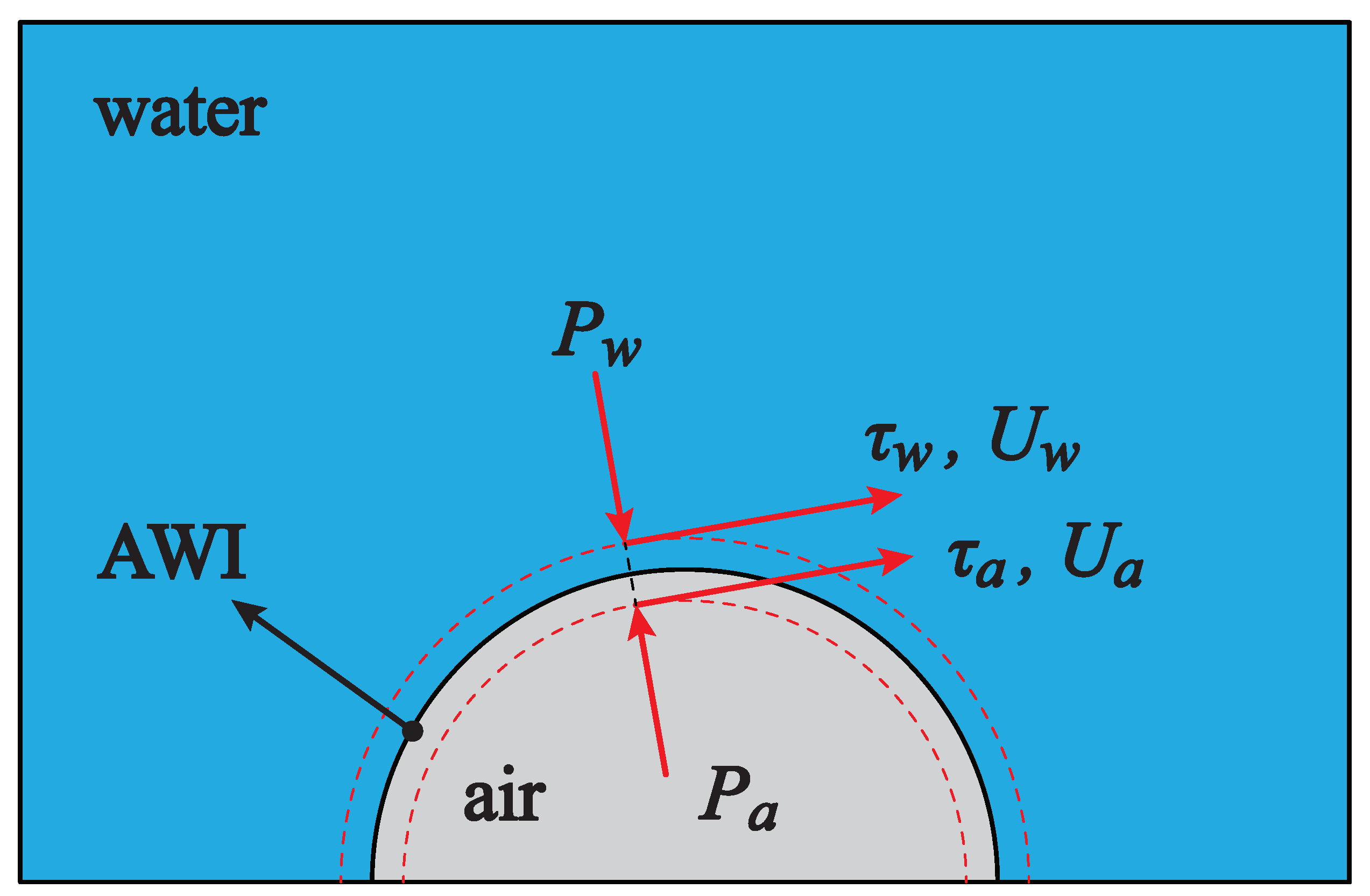
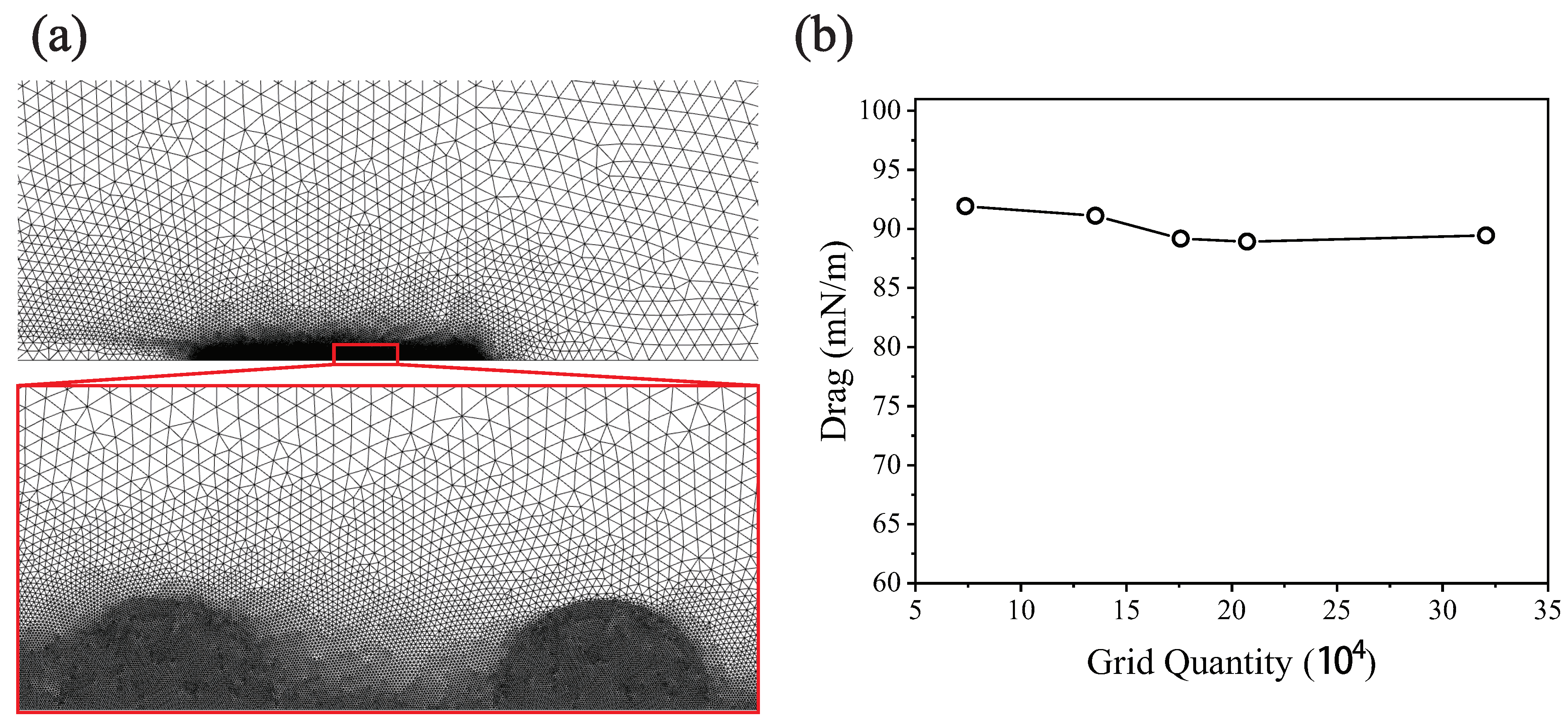
2.4. Numerical Method

Numerical simulation was performed with the Ansys Fluent 2021 R1. In order to simulate turbulent flow with low computational expense, the 2D standard k-$\epsilon$ model was used here. The governing equations are written as follows:

$${\displaystyle \frac{\partial \rho }{\partial t}}+\nabla ·\left(\rho \overrightarrow{v}\right)=0,$$

(1)

$${\displaystyle \frac{\partial \left(\rho \overrightarrow{v}\right)}{\partial t}}+\nabla ·\left(\rho \overrightarrow{v}\overrightarrow{v}\right)=-\nabla p+2\mu \nabla ·\mathbf{S},$$

(2)

$$\mathbf{S}={\displaystyle \frac{1}{2}}(\nabla \overrightarrow{v}+\nabla {\overrightarrow{v}}^T)-{\displaystyle \frac{1}{3}}\nabla ·v\mathbf{I},$$

(3)

where $\rho$, p, $\mu$ are the density, static pressure, and viscosity of the fluid, respectively. $\overrightarrow{v}$ is the velocity vector. $\mathbf{S}$ and $\mathbf{I}$ are the strain tensor and unit matrix, respectively. The transport equations for the standard k-$\epsilon$ model are written as follows:

$${\displaystyle \frac{\partial }{\partial t}}\left(\rho k\right)+\nabla ·\left(\rho k\overrightarrow{v}\right)=\nabla ·((\mu +{\displaystyle \frac{{\mu }_t}{{\sigma }_k}})\nabla ·k)+G_k-\rho \epsilon ,$$

(4)

$${\displaystyle \frac{\partial }{\partial t}}\left(\rho \epsilon \right)+\nabla ·\left(\rho \epsilon \overrightarrow{v}\right)=\nabla ·((\mu +{\displaystyle \frac{{\mu }_t}{{\sigma }_{\epsilon }}})\nabla ·\epsilon )+G_{\epsilon },$$

(5)

where k and $\epsilon$ are the turbulence kinetic energy and its rate of dissipation, respectively. $G_k$ and $G_{\epsilon }$ are added terms due to the generation of the turbulence kinetic energy. ${\mu }_{\tau }$ represents the turbulent viscosity. ${\sigma }_k$ and ${\sigma }_{\epsilon }$ are the turbulent Prandtl numbers for k and $\epsilon$, respectively.

The only model Ansys Fluent providing for the simulation of water flowing over air bubbles is the Volume of Fraction model, which can be coupled with the Level Set method. It is worth noting that the computation of Ansys Fluent is based on the control-volume formulation, and the surface tension is calculated as follows:

$$F_s=\sigma k_c\nabla \alpha ,$$

(6)

$$k_c=\nabla ·{\displaystyle \frac{\nabla \alpha }{∥\nabla \alpha ∥}},$$

(7)

where $\alpha$ is the volume fraction of one phase. In a real case, the grid is impossible to be fine enough to be isotropic. Thus, due to the anisotropy, there will be parasitic current and unwanted pressure gradient at the air–water interface (AWI).

In order to avoid the parasitic current and unwanted pressure gradient, an ideal lubricant interface model (ILIM) was proposed (Figure 5). The ILIM is based on four assumptions. The first assumption is that the adhering air bubble reaches a stable state and the AWI no longer transforms and moves. This assumption simplifies the model and helps the numerical work focusing on the slip effect and form effect of the adhering air bubble. The second assumption is that there is no mass transfer across the AWI. This assumption is naturally satisfied as air is almost immiscible in water. The third assumption is that the pressure drop across the AWI is balanced by the surface tension. The fourth assumption is that the shear stress and velocity are consecutive across the AWI. The third and fourth assumption are based on the balance force and no-slip boundary condition and can be written as follows:

$$(P_a-P_w)\overrightarrow{A}={\overrightarrow{F}}_s,$$

(8)

$${\overrightarrow{\tau }}_w={\overrightarrow{\tau }}_a,$$

(9)

$${\overrightarrow{U}}_w={\overrightarrow{U}}_a,$$

(10)

where P, $\overrightarrow{\tau }$, and $\overrightarrow{U}$ are the static pressure, shear stress, and velocity at the AWI, respectively. The subscript “w” and “a” denote the water side and the air side, respectively. The turbulent intensity at the velocity inlet is 5%. The ILIM was implemented through an user defined function.

The used domain for the simulation was a square two- dimensional region (Figure 6) with the leading part L1 = 300 mm, tailing part L2 = 200 mm, height H = 100 mm. It might be more suitable to apply a three-dimensional model. But, as clarified in Section 3.3, the grid quantity will exceed the affordable quantity. Thus, the two-dimensional model is applied here. In the middle of the leading part and tailing part, it was the bubbly region with adhering air bubbles (red hemi-circles in Figure 6). The total length of the bubbly region was 10 mm. The distance W between two adjacent bubbles was 1 mm. The inlet was a uniform velocity inlet. The outlet was pressure outlet. The shear stress of the upper wall was set to be 0 Pa. The lower wall was wall without slip. The enhanced wall treatment was applied here to make sure that the first layer of the grid with wall y* less than 11.25 could be solved.

3. Results and Discussion

3.1. The Result of Water Tunnel Experiment

The surface texture and wetting ability of the uncoated/coated microgrooves are presented in Figure 7. Before the dip-coating process, the microgrooves are smooth in the nanoscopic scale (Figure 7a) and is hydrophilic (Figure 7e). The hydrophilic surface is unable to trap air bubbles and the superhydrophobic coating is obtained by the dip-coating process (Figure 3). The dip-coating process uses the ethanol as a solvent due to its capability of dissolving the HSNPs and high volatility. The HSNPs are used as the superhydrophobic agent due to its super hydrophobicity. The microgrooves were immersed into the ethanol solution of the HSNPs and then lifted up. A thin liquid film of ethanol containing HSNPs formed on the microgrooves. After dried in an oven, the ethanol evaporated and left the HSNPs randomly accumulating in the microgrooves, forming a porous layer of HSNPs (Figure 7b,c).

From a large scale (Figure 7b) and a 3D perspective (Figure 7d), no cluster blocks the microgrooves. According to the 3D profile of the ZYGONexView, the depth of the coated grooves is about 9 µm. Comparing the depth of the coated grooves with the uncoated grooves, the difference means the thin layer of the HSNPs is about 1 µm thick and makes no change to the microscopic texture. After the dip-coating process, the coated microgrooves turns superhydrophobic and water droplets are repelled by it (Figure 7e). The static contact angle was measured with the OCA 25. The water contact angle (WCA) with the coated microgrooves in air is 148.5° (Figure 7f). The air contact angle (ACA) with the coated microgrooves in water is 60.3° (Figure 7g). The WCA and ACA mean that the coated microgrooves prefer to contact with air than water. The super hydrophobicity of the coated microgrooves guarantees that the microgrooves are filled with air during the hydrodynamic experiment.

In the water tunnel experiment, the bulk velocity varied from 0.50 m/s to 10.80 m/s. The smooth surface was used as the control sample, and the coated microgrooved surfaces were used as the experimental sample (Figure 8). The coated microgrooves were arranged in longitudinal direction (LS) and transverse direction (TS), respectively. The morphology of the adhering air bubbles on the sample LS and sample TS and its impact on the drag were tested in the water tunnel experiment by sticking the samples on the hydrofoil (Figure 4). For each sample, the morphology and the drag were recorded for three times.

The drag reduction rate $Dr$ of the sample LS and sample TS are presented in Figure 9. The $Dr$ is calculated as follows:

$$Dr=(1-{\displaystyle \frac{F}{F_s}})\times 100\%,$$

(11)

where the F and $F_s$ represent the drag of the experimental sample and the control sample, respectively. Both the sample LS and TS exhibit drag reduction performance at the velocity of 0.50 m/s. Then, both of them exhibit drag increase at the velocity around 0.93∼2.21 m/s. The drag increase reaches its maximum at the velocity of 1.36 m/s. The $Dr$ rises again when the velocity keeps increasing. The sample LS exhibits drag reduction at the velocity greater than 2.21 m/s, and the $Dr$ is around 3∼5%. The sample TS exhibits drag increase at the velocity greater than 2.21 m/s, and the $Dr$ is around −10%.

It is puzzling that both the sample LS and sample TS exhibit drag increase at the velocity around 0.93∼2.21 m/s. In order to explain the drag reduction performance of the experimental samples, the morphology of the adhering air bubbles are presented in Figure 10. The AWI can reflect light and is bright in the optical images. The air bubbles are pointed by white arrows in the optical images. It can be found that spherical air bubbles arise and adhere on both the sample LS and TS at the velocity of 0.5 m/s (Figure 10a,d). For the sample LS, the spherical air bubbles gradually disappear, and then banded bubbles arise when the velocity increases (Figure 10a–c). The spherical air bubbles gradually disappear and only the banded air bubbles are left at the velocity greater than 0.5 m/s. For the sample TS, the spherical air bubbles become smaller and smaller when the velocity increases (Figure 10d–f). The spherical air bubbles become invisible and is hard to be identified in the optical images at the velocity greater than 2.21 m/s.

According to the drag reduction performance and the morphology of the air bubbles, it is suspected that the spherical air bubbles cause the drag increase. It is shown in Figure 9 that both the sample LS and sample TS exhibit drag increase at the velocity around 0.93∼2.21 m/s. It is shown in Figure 10 that both the sample LS and sample TS are adhered by spherical air bubbles at the velocity around 0.93∼2.21 m/s. The similarity between the drag reduction performance and the air bubble morphology indicates that the spherical air bubbles are related to the drag increase. It is also shown in Figure 9 that the sample LS exhibits drag reduction while the sample TS exhibits drag increase at the velocity greater than 2.21 m/s. It is shown in Figure 10 that the sample LS is gradually adhered by banded air bubbles while the sample TS is still adhered by spherical air bubbles at the velocity greater than 0.5 m/s. The difference between the sample LS and sample TS indicates that the drag reduction in the sample LS is related to the banded air bubbles while the drag increase in the sample TS is related to the spherical air bubbles.

The size of the spherical air bubbles has influence on the drag and is presented in Figure 11. The size of the air bubbles is measured from the optical images shown in Figure 10. Because of the formation of the banded air bubbles on the sample LS, there are only diameters counted from the optical images obtained at the velocity of 0.50 m/s and 0.93 m/s. For the sample TS, the spherical bubbles are too small to be identified at the velocity greater than 2.21 m/s, and there are only diameters at the velocity less than 2.21 m/s. The diameter of the adhering spherical air bubbles decreases with the increasing velocity and varies from 0.09 mm to 0.31 mm (Figure 11a).

The diameter of the spherical air bubbles is compared with the viscous sublayer and is nondimensionalized with viscous length (Figure 11b). The dimensionless diameter $D^{+}$ is calculated as follows [7]:

$$D^{+}={\displaystyle \frac{D\sqrt{{\tau }_s/\rho }}{v}}={\displaystyle \frac{D\sqrt{F_s/\rho A}}{v}},$$

(12)

where the D, $\rho$, A, and v are the diameter of the spherical air bubble, the density of water, the total frictional area, and the kinematic viscosity of water. The dimensionless thickness of the viscous sublayer is 5, and the viscous force dominates in this layer. Out of this layer, the inertia force gradually dominates. It is shown in Figure 11b that the dimensionless diameter of the spherical air bubbles is around 13.6∼22.6, which is almost 2.7 times the thickness of the viscous sublayer. This indicates that the spherical air bubbles protrude out of the viscous sublayer and might block the flow in the boundary layer. Thus, the drag increase caused by the spherical air bubbles might be related with the pressure drag. It can also be found in Figure 11b that both the drag increase and $D^{+}$ reach the maximum at the velocity of 1.36 m/s. This confirms our suspicion that the drag increase is caused by the spherical air bubbles.

3.2. The Result of Towing Tank Experiment

In an attempt to obtain drag reduction with the superhydrophobic surface, a boat with a smooth surface and a boat with longitudinal microgrooves and hydrophobic coating were examined in the towing tank experiment. The width, depth, and length of the towing tank were 7 m, 7 m, and 435 m, respectively. The length and maximum width of the boats were about 8 m and 0.4 m, respectively. The longitudinal microgrooves (Figure 1) were printed onto the boat surface (Figure 12a). In the water tunnel experiment, the sample is small, and the hydrophobic coating is prepared by the dip-coating process. However, for the boat surface, it is technically difficult to use the dip-coating process, and the hydrophobic coating is sprayed onto the boat surface.

During the towing tank experiment, we found that the superhydrophobic boat surface is adhered by spherical air bubbles (Figure 12c) and only exhibits a drag reduction rate of 1% at the velocity of 1 m/s. At the velocity greater than 1 m/s, the drag reduction rate is around −3% (Figure 12d). The drag reduction rate $Dr$ slightly increases when the velocity increases. This result is similar to the sample TS in the water tunnel experiment. Our suspicion is that the drag increase is also related with the spherical air bubbles.

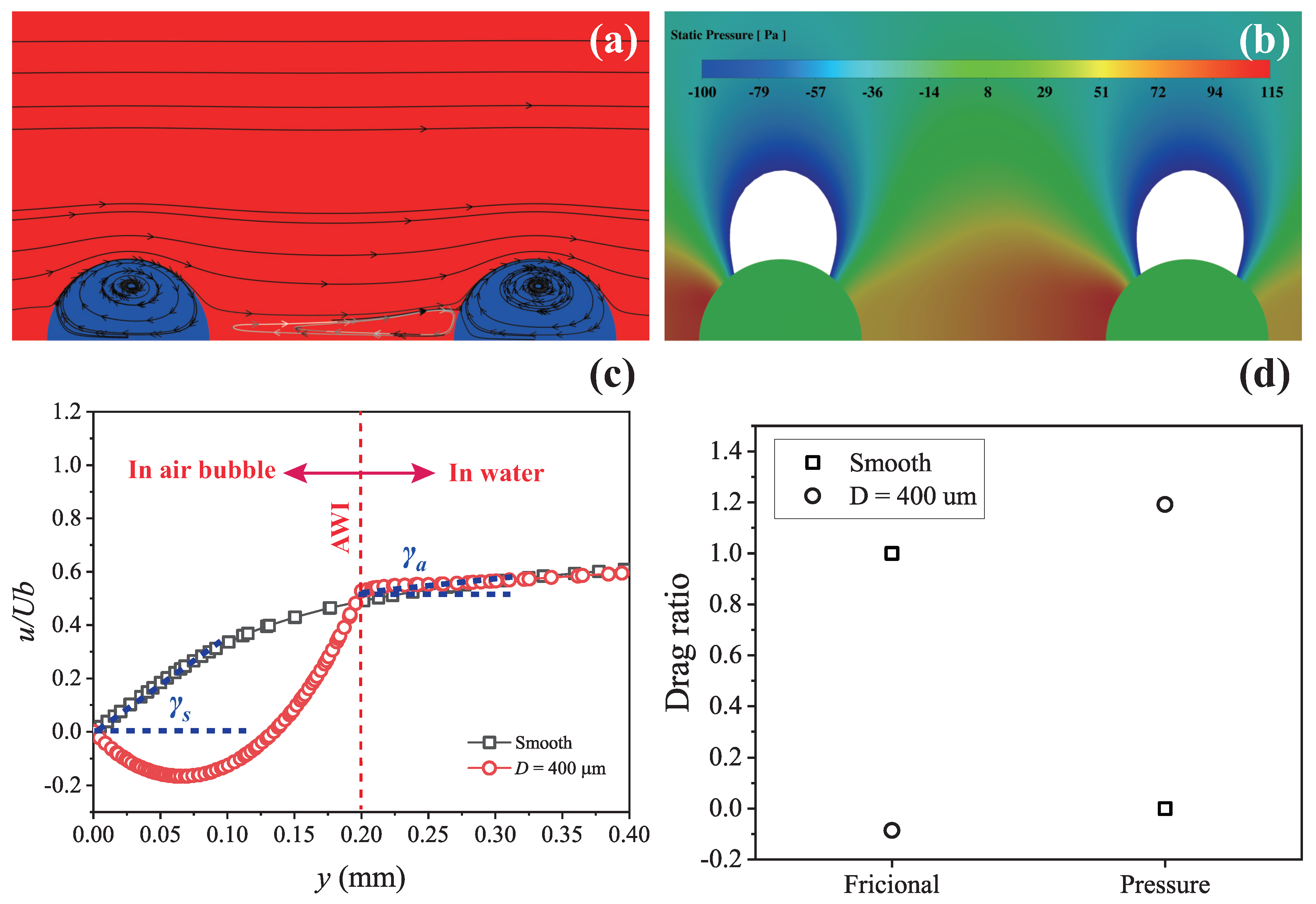
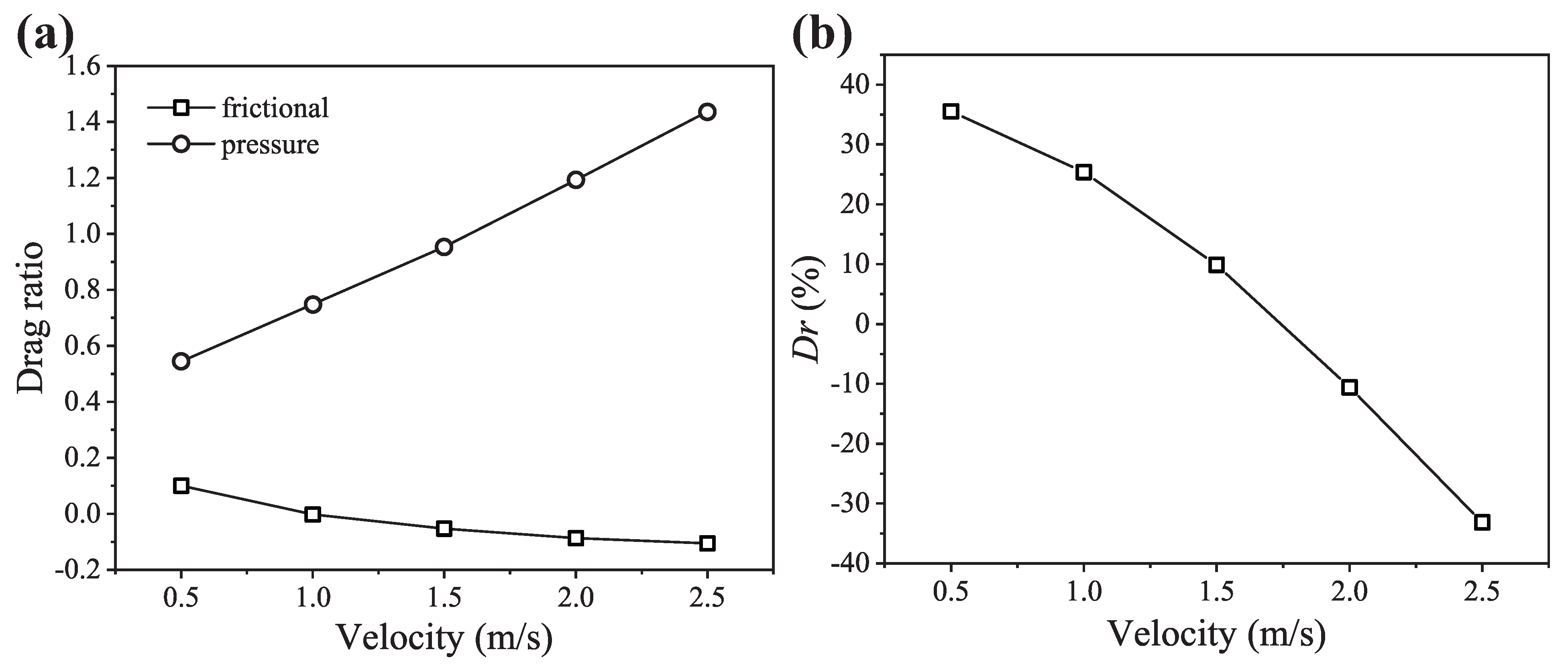
3.3. The Results of Numerical Simulation

In order to verify our suspicions and reveal the drag increase mechanism, the numerical simulation is conducted. The computational domain used in this simulation is shown in Figure 6. The total length and height of the domain are 510 mm and 100 mm, respectively. The diameter of the spherical air bubbles varies from 50 µm to 500 µm. Fine enough grids guarantee the accuracy of the calculated drag but cost much computational resource. In order to obtain accurate drag with acceptable computational expense, the computational domain was meshed into 1 mm triangular facets and refined around the bubbly region (Figure 13a).

In order to guarantee that the computational solution is independent with the grid quantity, the drag of the spherical air bubbles with diameter of 500 µm was calculated at the inlet velocity of 2 m/s and grid quantity varying from 73,600 to 321,000 (Figure 13b). The result shows that the grid quantity greater than 176,000 has little impact on the drag, confirming the grid independence. In this work, the grid quantity of 321,000 is chosen. The grid quantity of 321,000 instead of smaller grid quantity is chosen in order to guarantee the grid quality for the bubble diameter of 50 µm.

In Figure 14, the influence of the spherical air bubbles with diameter of 400 µm on the flow field at the velocity of 2 m/s are presented. It is shown in Figure 14a that the spherical air bubbles block the water flow around them and force the pathline to turn upward. Vortexes occur in the spherical air bubbles and the near wall region between the adjacent air bubbles. Because of the blockage of the spherical air bubbles, there exists pressure difference around the air bubbles (Figure 14b). The upstream pressure is higher than the downstream pressure, which indicates pressure drag. In Figure 14c, the x component of the velocity along the y axis shows that the velocity gradient near the smooth surface is greater than that near the AWI. The decrease in the velocity gradient means that the air bubbles can reduce the frictional drag. This is because that the viscosity of air is much smaller than that of water, and the frictional drag is proportional to the fluid viscosity. Thus, the air bubbles adhering on the surface can reduce the frictional drag.

In Figure 14d, the drag ratio of the drag component (the frictional drag and pressure drag) is plotted. The drag ratio is calculated as follows:

$$Dragratio={\displaystyle \frac{Dragcomponent}{Totaldragofsmoothsurface}}.$$

(13)

For the smooth surface, the surface is flat and the drag ratio of the pressure drag and frictional drag are 0 and 1, respectively. For the surface adhered with spherical air bubbles, the drag ratio of the pressure drag and frictional drag are −0.09 and 1.19, which means a drag increase of 10%. The frictional drag ratio of −0.09 confirms that the spherical air bubbles can effectively reduce frictional drag, which is the cause of the drag reduction in the sample LS and sample TS in the water tunnel experiment. The pressure drag ratio of 1.19 means pressure drag is introduced by the spherical air bubbles and explains the drag increase in the sample LS and sample TS in the water tunnel experiment. This result confirms our suspicion that spherical air bubbles adhering to the superhydrophobic surface will cause drag increase. The drag increase mechanism is that the adhering air bubbles not only reduce frictional drag but also introduce pressure drag and the introduced pressure drag exceeds the reduced frictional drag.

For a specific air bubble diameter of 400 µm, the influence of the air bubbles on the frictional drag and pressure drag at different velocity is presented in Figure 15. It is found in Figure 15a that the drag ratio of the pressure drag increases while the drag ratio of the frictional drag decreases when the velocity increases. This indicates that both the reduced frictional drag and introduced pressure drag increase when the velocity increase. It is also found in Figure 15a that the increasing speed of the introduced pressure drag is higher than the decreasing speed of the frictional drag. This implies that the spherical air bubbles exhibit drag reduction at low velocity but drag increase at high velocity. The drag reduction rate $Dr$ is plotted in Figure 15b. This result confirms that the spherical air bubbles can exhibit drag reduction at low velocity but will cause drag increase at high velocity. This result also explains the drag reduction in the sample LS and sample TS in the water tunnel experiment at the velocity of 0.5 m/s.

For a specific velocity of 2 m/s, the influence of the air bubble diameter on the frictional drag and pressure drag is presented in Figure 16. It is found in Figure 16a that the drag ratio of the pressure drag increases while the drag ratio of the frictional drag decreases when the air bubble diameter increases. This indicates that large air bubble not only reduce more frictional drag but also cause more pressure drag. In Figure 16b, the drag reduction rate $Dr$ is plotted. The result shows that the drag reduction rate first increases then decreases when the air bubble diameter increases.

4. Conclusions

In this work, the underwater drag reduction failure caused by the spherical air bubbles adhering to the superhydrophobic surface is reported, and the drag increase mechanism is revealed through the numerical simulation. In the water tunnel experiment, the superhydrophobic surface exhibits drag reduction of 20∼40% at the velocity of 0.5 m/s. The drag reduction turns to the drag increase of 10∼20% at the velocity 1.36 m/s. According to the optical images of the air bubbles adhering on the superhydrophobic surface, the drag increase is related to the spherical air bubbles. In the towing tank experiment, the superhydrophobic surfaces exhibited drag reduction at the velocity of 1 m/s. The drag reduction turns to the drag increase when the surfaces were adhered by spherical air bubbles. The numerical simulation indicates that the adhering spherical air bubbles not only reduce frictional drag but also introduce pressure drag. The drag increase is produced when the introduced pressure drag exceeds the reduced frictional drag. The numerical simulation also indicates that the reduced frictional drag and introduced pressure drag increase when the size of the spherical air bubbles or the velocity increases. But, the increasing speed of the introduced pressure drag is higher than that of the reduced frictional drag. This means that the spherical air bubbles only produce drag reduction when the bubble size or the velocity is small. This work might be helpful for researchers who are seeking for a drag reduction application of the superhydrophobic surface.

References

1. Zhang, X.; Zhang, D.Y.; Pan, J.F.; Li, X.; Chen, H.W. Controllable Adjustment of Bio-Replicated Shark Skin Drag Reduction Riblets. Appl. Mech. Mater. 2013, 461, 677–680. [Google Scholar] [CrossRef]
2. Walsh, M.J.; Weinstein, L.M. Drag and heat-transfer characteristics of small longitudinally ribbed surfaces. AIAA J. 1979, 17, 770–771. [Google Scholar] [CrossRef]
3. Choi, K.S.; Clayton, B.R. The mechanism of turbulent drag reduction with wall oscillation. Int. J. Heat Fluid Flow 2001, 22, 1–9. [Google Scholar] [CrossRef]
4. Gatti, D.; Guttler, A.; Frohnapfel, B.; Tropea, C. Experimental assessment of spanwise-oscillating dielectric electroactive surfaces for turbulent drag reduction in an air channel flow. Exp. Fluids 2015, 56, 110. [Google Scholar] [CrossRef]
5. Rajappan, A.; McKinley, G.H. Cooperative drag reduction in turbulent flows using polymer additives and superhydrophobic walls. Phys. Rev. Fluids 2020, 5, 114601. [Google Scholar] [CrossRef]
6. Fichman, M.; Hetsroni, G. Electrokinetic aspects of turbulent drag reduction in surfactant solutions. Phys. Fluids 2004, 16, 4346–4352. [Google Scholar] [CrossRef]
7. Bidkar, R.A.; Leblanc, L.; Kulkarni, A.J.; Bahadur, V.; Ceccio, S.L.; Perlin, M. Skin-friction drag reduction in the turbulent regime using random-textured hydrophobic surfaces. Phys. Fluids 2014, 26, 18. [Google Scholar] [CrossRef]
8. Xu, M.; Yu, N.; Kim, J.; Kim, C.J.C. Superhydrophobic drag reduction in high-speed towing tank. J. Fluid Mech. 2020, 908, A6. [Google Scholar] [CrossRef]
9. Kim, H.N.; Kim, S.J.; Choi, W.; Sung, H.J.; Lee, S.J. Depletion of lubricant impregnated in a cavity of lubricant-infused surface. Phys. Fluids 2021, 33, 022005. [Google Scholar] [CrossRef]
10. Yao, W.H.; Wu, L.; Sun, L.D.; Jiang, B.; Pan, F.S. Recent developments in slippery liquid-infused porous surface. Prog. Org. Coat. 2022, 166, 106806. [Google Scholar] [CrossRef]
11. Tong, W.; Xiong, D.S.; Zhou, H.J. TMES-modified SiO2 matrix non-fluorinated superhydrophobic coating for long-term corrosion resistance of aluminium alloy. Ceram. Int. 2020, 46, 1211–1215. [Google Scholar] [CrossRef]
12. Guo, D.Y.; Chen, J.H.; Wen, L.F.; Wang, P.; Xu, S.P.; Cheng, J.; Wen, X.F.; Wang, S.F.; Huang, C.Y.; Pi, P.H. A superhydrophobic polyacrylate film with good durability fabricated via spray coating. J. Mater. Sci. 2018, 53, 15390–15400. [Google Scholar] [CrossRef]
13. Zhang, Y.; Wang, T.; Lv, Y.J. Durable Biomimetic Two-Tier Structured Superhydrophobic Surface with Ultralow Adhesion and Effective Antipollution Property. Langmuir 2023, 39, 2548–2557. [Google Scholar] [CrossRef] [PubMed]
14. Hu, Y.M.; Zhu, Y.; Zhou, W.; Wang, H.; Yi, J.H.; Xin, S.S.; He, W.J.; Shen, T. Dip-coating for dodecylphosphonic acid derivatization on aluminum surfaces: An easy approach to superhydrophobicity. J. Coat. Technol. Res. 2016, 13, 115–121. [Google Scholar] [CrossRef]
15. Celik, N.; Torun, I.; Ruzi, M.; Esidir, A.; Onses, M.S. Fabrication of robust superhydrophobic surfaces by one-step spray coating: Evaporation driven self-assembly of wax and nanoparticles into hierarchical structures. Chem. Eng. J. 2020, 396, 125230. [Google Scholar] [CrossRef]
16. Zhang, L.S.; Zhou, A.G.; Sun, B.R.; Chen, K.S.; Yu, H.Z. Functional and versatile superhydrophobic coatings via stoichiometric silanization. Nat. Commun. 2021, 12, 982. [Google Scholar] [CrossRef]
17. Chen, X.Y.; Yuan, J.H.; Huang, J.; Ren, K.; Liu, Y.; Lu, S.Y.; Li, H. Large-scale fabrication of superhydrophobic polyurethane/nano-Al2O3 coatings by suspension flame spraying for anti-corrosion applications. Appl. Surf. Sci. 2014, 311, 864–869. [Google Scholar] [CrossRef]
18. Barbier, C.; Jenner, E.; D’Urso, B. Drag reduction with superhydrophobic riblets. In Proceedings of the ASME International Mechanical Engineering Congress and Exposition, Houston, TX, USA, 9–15 November 2012; pp. 199–205. [Google Scholar]
19. Chen, Q.D.; Duan, J.; Hou, Z.B.; Hou, G.X.; Deng, L.M. Effect of the surface pattern on the drag property of the superhydrophobic surface. Phys. Fluids 2022, 34, 114113. [Google Scholar] [CrossRef]
20. Saranadhi, D.; Chen, D.Y.; Kleingartner, J.A.; Srinivasan, S.; Cohen, R.E.; McKinley, G.H. Sustained drag reduction in a turbulent flow using a low-temperature Leidenfrost surface. Sci. Adv. 2016, 2, 9. [Google Scholar] [CrossRef]
21. Aljallis, E.; Sarshar, M.A.; Datla, R.; Sikka, V.; Jones, A.; Choi, C.H. Experimental study of skin friction drag reduction on superhydrophobic flat plates in high Reynolds number boundary layer flow. Phys. Fluids 2013, 25, 14. [Google Scholar] [CrossRef]
22. Gose, J.W.; Golovin, K.; Boban, M.; Mabry, J.M.; Tuteja, A.; Perlin, M.; Ceccio, S.L. Characterization of superhydrophobic surfaces for drag reduction in turbulent flow. J. Fluid Mech. 2018, 845, 560–580. [Google Scholar] [CrossRef]
23. Ling, H.; Srinivasan, S.; Golovin, K.; McKinley, G.H.; Tuteja, A.; Katz, J. High-resolution velocity measurement in the inner part of turbulent boundary layers over super-hydrophobic surfaces. J. Fluid Mech. 2016, 801, 670–703. [Google Scholar] [CrossRef]
24. Abu Rowin, W.; Ghaemi, S. Streamwise and spanwise slip over a superhydrophobic surface. J. Fluid Mech. 2019, 870, 1127–1157. [Google Scholar] [CrossRef]
25. Abu Rowin, W.; Ghaemi, S. Effect of Reynolds number on turbulent channel flow over a superhydrophobic surface. Phys. Fluids 2020, 32, 075105. [Google Scholar] [CrossRef]
26. Reholon, D.; Ghaemi, S. Plastron morphology and drag of a superhydrophobic surface in turbulent regime. Phys. Rev. Fluids 2018, 3, 104003. [Google Scholar] [CrossRef]
27. Park, H.; Sun, G.; Kim, C.J. Superhydrophobic turbulent drag reduction as a function of surface grating parameters. J. Fluid Mech. 2014, 747, 722–734. [Google Scholar] [CrossRef]
Figure 1. The surface texture before the hydrophobic coating.
Jmse 12 02170 g001
Figure 2. The dip-coating process.
Jmse 12 02170 g002
Figure 3. Hydrodynamic experimental apparatus. Full view (a) and test section (b) of the water tunnel. The structure of the force transducer (c), the placement of the high-resolution camera (d), and its record part (e).
Jmse 12 02170 g003
Figure 4. Flexible PE film was stuck onto the hydrofoil.
Jmse 12 02170 g004
Figure 5. Schematic diagram of the ILIM.
Jmse 12 02170 g005
Figure 6. Schematic diagram of the 2D domain for the simulation.
Jmse 12 02170 g006
Figure 7. Images of surface texture and wetting ability. SEM image (a) for uncoated microgrooves and (b,c) for coated microgrooves; (d) is the 3D profile of the coated microgrooves; (e) for dyed water droplets on uncoated surface and coated microgrooves; (f) for the WCA with the coated microgrooves in air; (g) for the ACA with the coated microgrooves in water.
Jmse 12 02170 g007
Figure 8. The schematic of the smooth surface and LS and TS.
Jmse 12 02170 g008
Figure 9. The drag reduction rate D r for the sample LS and sample TS.
Jmse 12 02170 g009
Figure 10. Optical images of the morphology of the adhering air bubbles on the sample LS and sample TS. (af) are images obtained in the stream-wise normal plane. The location of the sample is represented by the green dashed line. The hydrofoil is above this line, and the water is below this line. The red scale bar is 1 mm. (ac) for LS and (df) for TS. (a,d), (b,e), (c,f) are recorded at the velocity of 0.50 m/s, 1.36 m/s, and 2.21 m/s, respectively. (g,h) are recorded videos (MP4 file) for the sample LS and sample TS at the velocity of 2.21 m/s, respectively.
Jmse 12 02170 g010
Figure 11. The diameter (a) and dimensionless diameter D + (b) of the spherical air bubbles on the sample LS and sample TS.
Jmse 12 02170 g011
Figure 12. (a) is the process of printing the microgrooves onto the boat surface. (b) is the boat prepared for the towing tank experiment. (c) is the adhering air bubbles on the boat surface. (d) is the drag reduction rate.
Jmse 12 02170 g012
Figure 13. Grids of the computational domain (a) and verification of the grid independence (b).
Jmse 12 02170 g013
Figure 14. The influence of the spherical air bubbles with diameter of 400 µm on the flow field at the velocity of 2 m/s. (a) is the pathline, (b) is the static pressure, (c) is the velocity profile along y axis, and (d) is the drag ratio. The red color and blue color in (a) represent water and air, respectively. The white holes in (b) represent static pressure lower than −100 Pa. The static pressure here is calculated as the difference between the actual static pressure and the reference pressure (1 atm).
Jmse 12 02170 g014
Figure 15. Variation in the drag ratio (a) and drag reduction rate D r (b) with the velocity.
Jmse 12 02170 g015
Figure 16. Variation in the drag ratio (a) and drag reduction rate D r (b) with the air bubble diameter.
Jmse 12 02170 g016
Disclaimer/Publisher’s Note: The statements, opinions and data contained in all publications are solely those of the individual author(s) and contributor(s) and not of MDPI and/or the editor(s). MDPI and/or the editor(s) disclaim responsibility for any injury to people or property resulting from any ideas, methods, instructions or products referred to in the content.