A Fast Adaptive AUV Control Policy Based on Progressive Networks with Context Information

Abstract

Deep reinforcement learning models have the advantage of being able to control nonlinear systems in an end-to-end manner. However, reinforcement learning controllers trained in simulation environments often perform poorly with real robots and are unable to cope with situations where the dynamics of the controlled object change. In this paper, we propose a DRL control algorithm that combines progressive networks and context as a depth tracking controller for AUVs. Firstly, an embedding network that maps interaction history sequence data onto latent variables is connected to the input of the policy network, and the context generated by the network gives the DRL agent the ability to adapt to the environment online. Then, the model can be rapidly adapted to a new dynamic environment, which was represented by the presence of generalized force disturbances and changes in the mass of the AUV, through a two-stage training mechanism based on progressive neural networks. The results showed that the proposed algorithm was able to improve the robustness of the controller to environmental disturbances and achieve fast adaptation when there were differences in the dynamics.

1. Introduction

As marine exploration develops,  AUVs are being used for a variety of tasks, including marine surveys, demining, and bathymetry data collection in marine and riverine environments [1]. AUV trajectory tracking control is a prerequisite for achieving most advanced tasks. However, the actual operating scenarios of AUVs are usually complex, diverse, and unpredictable. The tracking controller will be affected by highly nonlinear vehicle dynamics and external time-varying disturbances. These effects make the dynamics of an AUV difficult to measure or difficult to measure in the underwater environments being investigated, causing various uncertainties [2]. Therefore, designing a robust AUV tracking controller is a meaningful and challenging problem.

In previous studies, model-based control methods have been widely adopted due to their intuitiveness and reliability. Yang et al. combined neural networks and AUV control to realize AUV adaptive terminal sliding mode trajectory tracking [3]. The work of Khodayari et al. [4] combined fuzzy control and a PID controller; used Mamdani fuzzy rules to adjust PID parameters; and applied this to speed, depth, and heading control. Liang et al. [5] proposed an adaptive robust control system using backstepping and sliding mode control, realizing AUV three-dimensional path tracking under the conditions of parameter uncertainty and external interference. Zhang et al. transformed the tracking control problem into a standard convex quadratic programming problem that is easy to calculate online, and designed a tracking controller based on the model predictive control (MPC) method. Simulations were conducted under two different three-dimensional trajectories to verify the feasibility and robustness of the algorithm. The design of the above method relies on accurate AUV dynamic and kinematic models. The control performance depends on the accuracy of the model. When there are errors in the model, the control performance will significantly decrease.

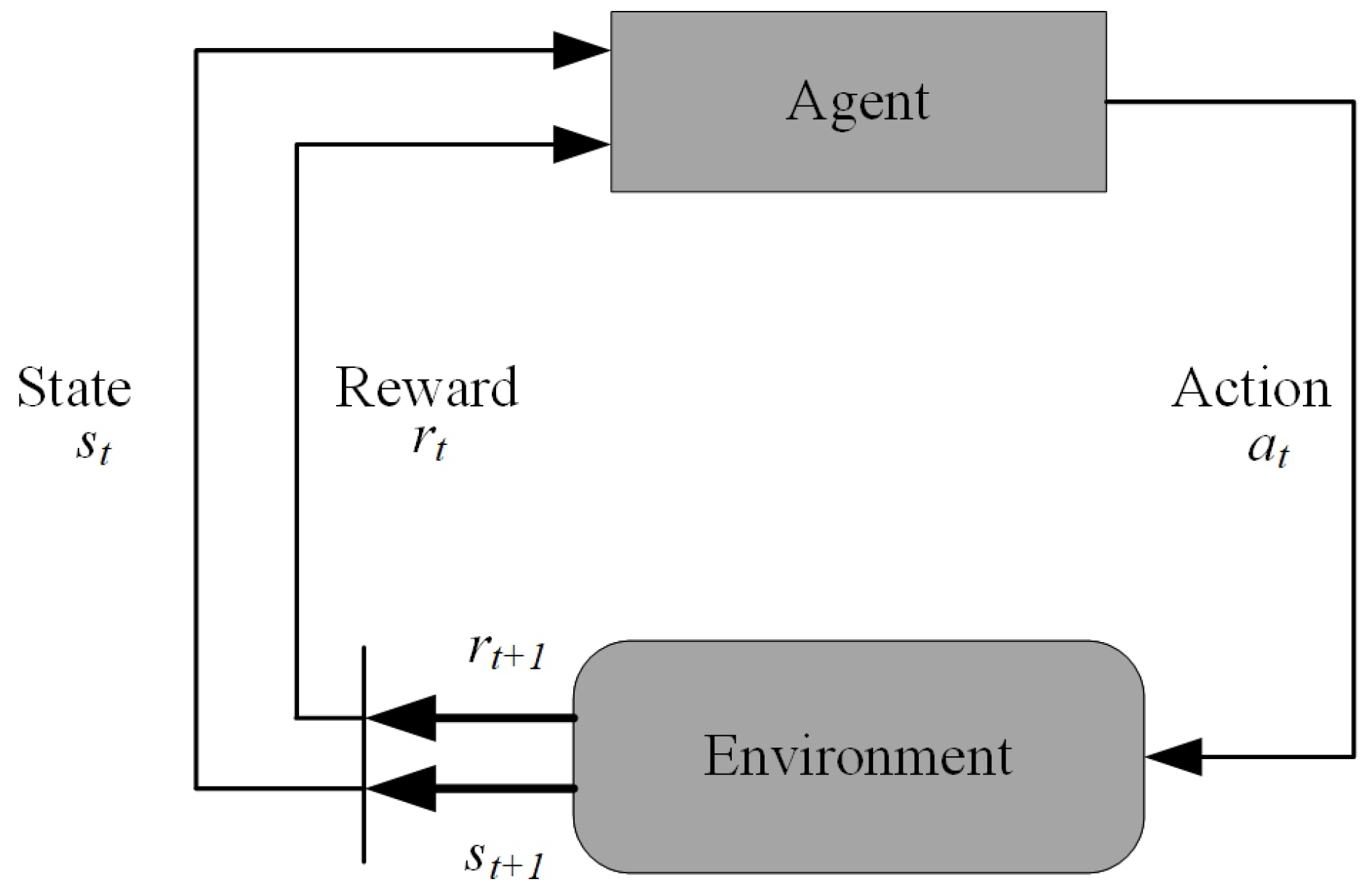
In recent years, deep reinforcement learning (DRL) [6], as an emerging method for solving optimal control problems for nonlinear systems, has shown great potential for a variety of robot control tasks, such as underwater robots and unmanned aerial vehicles. Compared with traditional controllers, DRL has less precise requirements for system modeling, and the controller converges through interaction with and exploration of the environment. Wu et al. [7] proposed a DRL controller based on the deterministic policy gradient theorem, which showed better results than nonlinear model predictive control (NMPC) and linear quadratic Gaussian (LQG) methods in experiments. Sun et al. [8] designed a three-dimensional path tracking controller based on the deep deterministic policy gradient (DDPG) algorithm, and effectively reduced the steering frequency by using the rudder angle and its change rate as new terms in the reward function. Furthermore, in order to enable the controller to observe ocean current disturbances and adjust output, an ocean current disturbance observer was proposed. Du et al. [9] proposed a DRL control strategy based on a reference model, introducing a reference model into the actor–critic structure to provide a smoothed reference target for the DRL model, giving the controller improved robustness, while eliminating response overshoot and control command saturation. When training DRL-based reinforcement learning controllers, there may be sparse reward and local convergence issues. Mao et al. [10] proposed a multi-agent GAIL (MAG) algorithm based on generative adversarial imitation, enabling AUVs to overcome the difficulty of slow initial training of a network. Shi et al. [11] improved experience replay rules and used an experience replay buffer to store and destroy samples, so that time series samples could be used to train neural networks. Experimental results showed that the algorithm had a fast and stable learning effect. Palomeras et al. [12] proposed an AUV control architecture and used an actor–critic reinforcement learning algorithm in the reaction layer. The AUV using this control structure successfully completed vision-based cable following in a real scenario. Meanwhile, Liu et al. [13] modeled a pipeline following problem as an end-to-end mapping from an image to AUV velocity, and used proximal policy optimization (PPO) to train their network. However, most current DRL methods only conduct training in an ideal simulation environment, ignoring the dynamic differences between a training environment and a working environment. An AUV is a nonlinear time-varying system, and the underwater environment has a fluid force interferences that is difficult to model. Therefore, the performance of models trained in simulation environments often decreases in the real environments, which is called the “reality gap” [14].

In order to close this gap, domain randomization has become a common approach, i.e., randomizing certain parameters of the training environment during training. For example, Peng et al. [15] randomly selected several environmental parameters at the beginning of each round of training: connecting rod mass, joint damping, ice hockey mass, table height, etc. Andrychowicz et al. [16] not only randomized the physical parameters in a simulation environment, but also modeled additional effects specific to the robotic arm and accelerated policy convergence through large-scale distributed training. Tan et al. [17] believed that the information transmission delay that exists in reality but does not exist in a simulation is the reason for the oscillation of a simulation strategy in a real environment, and this delay was also simulated. The parameter range of the domain randomization method relies on artificial prior knowledge. The wider the parameter range, the more robust the strategy, and the worse the control performance; therefore, domain randomization is a compromise that trades optimality for robustness. Another common way to overcome the reality gap is to introduce context into a DRL model. Yu et al. [18] utilized a fully connected network to map recent interaction history sequence data into model parameters, and used the network output as part of the DRL model input. Zhou et al. [19] used an interaction strategy alone to interact with the environment to generate the most informative trajectory. Ball et al. [20] defined context variables as the ratio of state changes and implemented online context learning through a simple linear model, allowing the algorithm to be generalized to environments with changing dynamics. Compared with domain randomization, context-based methods can achieve online adaptation to an environment, but parameters such as the scope of the training environment and the length of the context need to be measured experimentally to accurately represent the real environment. The model performance still relies on human priors. Rusu et al. [21] proposed a progressive neural network (PNN), which uses a laterally connected network architecture to extract correlations between tasks, effectively improving the training efficiency while avoiding catastrophic forgetting, and applied it to a pixel-driven robot control problem [22]. However, the number of parameters of the PNN increases as the amount of tasks increases, and it is suitable for migration tasks between a small number of static environment tasks in the field of robot control. Each of the above methods has certain drawbacks, and they have been little applied in the field of AUV control.

To solve the above problems, this study combines the context concept and a PNN structure with the DRL algorithm, takes the context generated by embedding networks as part of the input to the policy network, and performs two-stage training based on the PNN architecture, so that the proposed method has the dual advantages of robustness to disturbances and fast adaptation. The main contributions of this study are as follows.

• Context is introduced into the DRL controller through embedding networks. In the decision-making process, the embedding networks map the interaction history sequences onto latent variables representing the context, thus taking the current environment information as part of the decision-making factors, which gives the model the ability to adapt to the environment online.
• A PNN-based training architecture is formulated. The DRL model utilizes the PNN’s property of lateral connectivity to quickly adapt to new working environments and transfer between different dynamical environments.
• Several experiments were designed to validate the performance of the proposed method. These included tracking experiments for step signals, robustness experiments for various external disturbances, and adaptability experiments where the dynamics were changed.

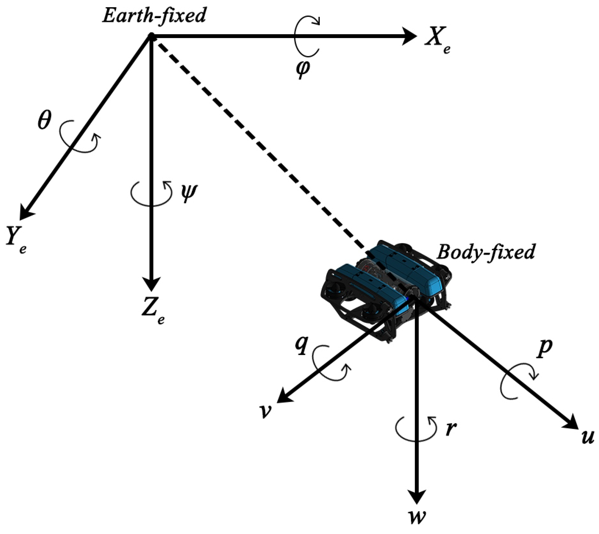
The rest of this paper is organized as follows: Section 2 presents the mathematical equations for the kinematics and dynamics model of the AUV system and briefly introduces the PPO model; Section 3 explains the structure and flow of the proposed algorithm; Section 4 presents the results of testing the proposed method in various environments and comparing the results with the results of the other algorithms; and, finally, Section 5 gives the conclusions and an outlook for the future.

2. Problem Formulation

2.1. Coordinate Systems of AUVs

The motion description of AUVs involves two sets of coordinates [23], namely the Earth-fixed coordinate frame and the body-fixed coordinate frame, as shown in Figure 1.

The absolute position of an AUV is described by $\eta ={[X,Y,Z,\phi ,\theta ,\psi ]}^T$, where ${\eta }_2={[\phi ,\theta ,\psi ]}^T$ represent the roll angle, pitch angle, and yaw angle of the AUV, respectively, and ${\eta }_1={[X,Y,Z]}^T$ represents the position of the AUV in the inertial coordinate system. The velocity vector is described by $v={[u,v,w,p,q,r]}^T$, where $v_1={[u,v,w]}^T$ represent surge, sway, and heave velocity, and $v_2={[p,q,r]}^T$ represent the roll, pitch, and yaw angular velocity. The motion relationship between the Earth-fixed coordinate frame and the body-fixed coordinate frame of the AUV is

$$J=\left[\begin{array}{c}J\left({\eta }_1\right)\\ J\left({\eta }_2\right)\end{array}\right]$$

(1)

$$\dot{\eta }=J\left({\eta }_2\right)\dot{v}$$

(2)

$$J_1\left({\eta }_2\right)=\left[\begin{array}{ccc}\cos \psi \cos \theta & -\sin \psi \cos \phi +\cos \psi \sin \theta \sin \phi & \sin \psi \sin \phi +\cos \psi \cos \phi \sin \theta \\ \sin \psi \cos \theta & \cos \psi \cos \phi +\sin \phi \sin \theta \sin \psi & -\cos \psi \sin \phi +\sin \theta \sin \psi \cos \phi \\ -\sin \theta & \cos \theta \sin \phi & \cos \theta \cos \phi \end{array}\right]$$

(3)

$$J_2\left({\eta }_2\right)=\left[\begin{array}{ccc}1& \sin \phi \tan \theta & \cos \phi \tan \theta \\ 0& \cos \phi & -\sin \phi \\ 0& {\displaystyle \frac{\sin \phi }{\cos \theta }}& {\displaystyle \frac{\cos \phi }{\cos \theta }}\end{array}\right]$$

(4)

The mathematical expression of the motion equation [24] of a six-degree-of-freedom AUV is

$$M\dot{v}=C\left(v\right)v+D\left(v\right)v+g\left(\eta \right)=\tau +{\tau }^{\prime }$$

(5)

$$M=M_{rb}+M_a$$

(6)

$$C\left(v\right)=C_{rb}\left(v\right)+C_a\left(v\right)$$

(7)

$$g\left(\eta \right)=\left[\begin{array}{c}(W-B)\sin \theta \\ -(W-B)\cos \theta \sin \phi \\ -(W-B)\cos \theta \cos \phi \\ -(y_{G}W-y_{G}B)\cos \theta \cos \phi +(z_{G}W-z_{B}B)\cos \theta \cos \phi \\ (z_{G}W-z_{B}B)\sin \phi +(x_{G}W-x_{B}B)\cos \theta \cos \phi \\ -(x_{G}W-x_{B}B)\cos \theta \sin \phi -(y_{G}W-y_{B}B)\sin \theta \end{array}\right]$$

(8)

Here, M represents the mass matrix, comprising both the rigid body mass matrix and the added masses specific to the AUV system. $C\left(n\right)$ denotes the Coriolis force matrix, encompassing both the Coriolis force matrix and the additional mass-induced Coriolis force matrix. $D\left(v\right)$ stands for the damping matrix. $g\left(\eta \right)$ is the reversion moment matrix, which consists of gravity W and buoyancy B. The vectors $r_G={[x_g,y_g,z_g]}^T$ and $r_B={[x_b,y_b,z_b]}^T$ represent the coordinates of the center of gravity and center of buoyancy, respectively. $\tau$ is the vector of forces and moments generated by the propeller, and ${\tau }^{\prime }$ is generalized forces generated by unknown factors such as environmental disturbances.

2.2. AUV Vertical Plane Target Tracking Task Description

Our definition of the target tracking task is similar to SHI et al. [11], who decomposed the AUV target tracking task into tracking tasks in the vertical plane and surge direction, as shown in Figure 2. In this study, we modeled the BlueROV Heavy developed by the American company BlueRobotics [4]. This vehicle can be viewed as an overdriven AUV system that can generate forces and moments in each of the six degrees of freedom by setting the thrust ratios of the eight thrusters. Without loss of generality, we investigated the tracking problem in the Y-Z vertical plane. In addition, we also made two reasonable assumptions based on the characteristics of the AUV used in our experiments:

(1)

The center of buoyancy of the underwater vehicle coincides with the center of gravity.

(2)

The AUV completes target tracking through translation in the sway direction and heave direction. Yaw, pitch, and roll motions are ignored during motion.

Based on the above assumptions, the motion equation of the AUV in the vertical plane can be expressed as

$$m\dot{v}=Y_{\left|v\right|v}v\left|v\right|+Y_{\dot{v}}\dot{v}+Y+Y^{\prime }$$

(9)

$$m\dot{w}=Z_{\left|w\right|w}w\left|w\right|+Z_{\dot{w}}\dot{w}+Z+Z^{\prime }$$

(10)

$$v=v+\dot{v}△t$$

(11)

$$w=w+\dot{w}△t$$

(12)

where $△t$ is the time interval, Y and Z are the thrust forces generated by the thruster in the sway direction and the heave direction, and $Y^{\prime }$ and $Z^{\prime }$ are the generalized forces on the AUV in the sway direction and the heave direction. The values of the hydrodynamic coefficient are shown in

Table 1. The nonlinear hydrodynamic coefficients of the AUV model.

Coefficient	Value
m (kg)	13.5
Z|w|w (kg/m)	190.0
Y|v|v (kg/m)	217.0
${\mathrm{Z}}_{\dot{w}}$ (kg)	18.68
${\mathrm{Y}}_{\dot{v}}$	7.12

.

2.3. DRL Algorithm PPO Description

Reinforcement learning is a machine learning method that maximizes rewards by learning policies during interaction with the environment. A common model of reinforcement learning is the Markov decision process (MDP). Its basic process can be described as follows: the agent perceives the current environmental state $S_t$ at time t, makes an action $a_t$ through a policy, and the action acts on the environment to cause a state transition to $S_{t+1}$. At the same time, the environment feeds back a reward value to the agent based on a potential reward function, as shown in Figure 3.

The goal of the MDP is to maximize the cumulative discount reward obtained by the policy ${\pi }_{\theta }$ in the environment. The optimization objective can be expressed as

$$\underset{\theta }{\max }J\left(\theta \right)=\underset{\theta }{\max }{E}_{\tau \sim {\pi }_{\theta }}R\left(\tau \right)=\underset{\theta }{\max }\sum _{\tau }P(\tau \mid \theta )R\left(\tau \right)$$

(13)

where $P(\tau \mid \theta )$ is the probability of the policy ${\pi }_{\theta }$ generating a trajectory $\tau$. Usually, for maximization problems, we can use a gradient ascent algorithm to find the maximum value:

$${\theta }^{*}=\theta +\alpha {\nabla }_{\theta }J\left({\pi }_{\theta }\right)$$

(14)

A policy gradient (PG) [25] is a type of reinforcement learning algorithm that directly models and optimizes policies. The basic idea is to increase the probability of choosing an action if it increases the cumulative reward, and to decrease the probability of choosing the action if it does not. The policy gradient functions by computing the derivatives of the objective function with respect to the policy parameters:

$${\nabla }_{\theta }J\left(\theta \right)=\underset{\tau \sim {\pi }_{\theta }}{E}\left[{\nabla }_{\theta }\log P(\tau \mid \theta )R\left(\tau \right)\right]=\underset{\tau \sim {\pi }_{\theta }}{E}\left[\sum _{t=0}^T{\nabla }_{\theta }\log {\pi }_{\theta }\left(a_t\mid s_t\right)R\left(\tau \right)\right]$$

(15)

The theoretical calculation formula of a policy gradient is a mathematical expectation. A specific implementation can adopt the Monte Carlo method; that is, sampling a large number of the trajectories of the interactions between the policy and the environment, and approximately expressing the expectation by averaging. A significant disadvantage of the PG method is that the data sampling efficiency is low. Every time a parameter is updated, the trajectory data need to be resampled, because the PG requires the same policy for sampling data as for updating parameters. Proximal policy optimization (PPO) [26] achieves data reuse through importance sampling, using a set of data to update model parameters multiple times. To ensure the effectiveness of importance sampling, PPO-clip limits the difference between old and new policies by performing a clipping operation on the objective function:

$$L\left(\theta \right)=E\left[\min \left(r_t\left(\theta \right)A\left(s_t,a_t\right),\mathrm{clip}\left(r_t\left(\theta \right),1-\epsilon ,1+\epsilon \right)A\left(s_t,a_t\right)\right)\right]$$

(16)

where $r_t\left(\theta \right)={\displaystyle \frac{{\pi }_{\theta }\left(a_t\mid s_t\right)}{{\pi }_{{\theta }_0}\left(a_t\mid s_t\right)}}$ represents the probability ratio, ${\pi }_{\theta }\left(a_t\mid s_t\right)$ and ${\pi }_{{\theta }_0}\left(a_t\mid s_t\right)$ are, respectively, the probability of action $a_t$ taken by the current policy ${\pi }_{\theta }$ and the data sampling policy ${\pi }_{{\theta }_0}$ when the agent is in the state $S_t$. $A\left(s_t,a_t\right)$ is the advantage function, which represents the relative advantage of receiving rewards for behavior $a_t$ in the state $S_t$. A critic network $V_{\varphi }$ is usually used to calculate generalized advantage estimation (GAE):

$$A\left(s_t,a_t\right)=r_t^r+\gamma V\left(s_{t+1}\right)-V\left(s_t\right)$$

(17)

The form of the clip function is

$$clip\left(r_t\left(\theta \right),1-\epsilon ,1+\epsilon \right)=\left\{\begin{array}{cc}1+\epsilon ,& r_t\left(\theta \right)\ge 1+\epsilon \hfill \\ 1-\epsilon ,& \left.r_t\left(\theta \right)\le 1-\epsilon \right)\hfill \\ r_t\left(\theta \right),& \mathrm{else}\hfill \end{array}\right.$$

(18)

When $A\left(s_t,a_t\right)$, the PPO-clip algorithm increases the probability ${\pi }_{\theta }\left(a_t\mid s_t\right)$ of this state–action pair through the optimization goal $L\left(\theta \right)$, but the probability ratio $r_t\left(\theta \right)$ will not exceed $1+\epsilon$. On the contrary, the PPO-clip algorithm reduces the probability ${\pi }_{\theta }\left(a_t\mid s_t\right)$ of this state–action pair through the optimization goal $L\left(\theta \right)$, but the probability ratio $r_t\left(\theta \right)$ will not be less than $1-\epsilon$.

3. Proposed Method

3.1. Context-Based Policy Architecture

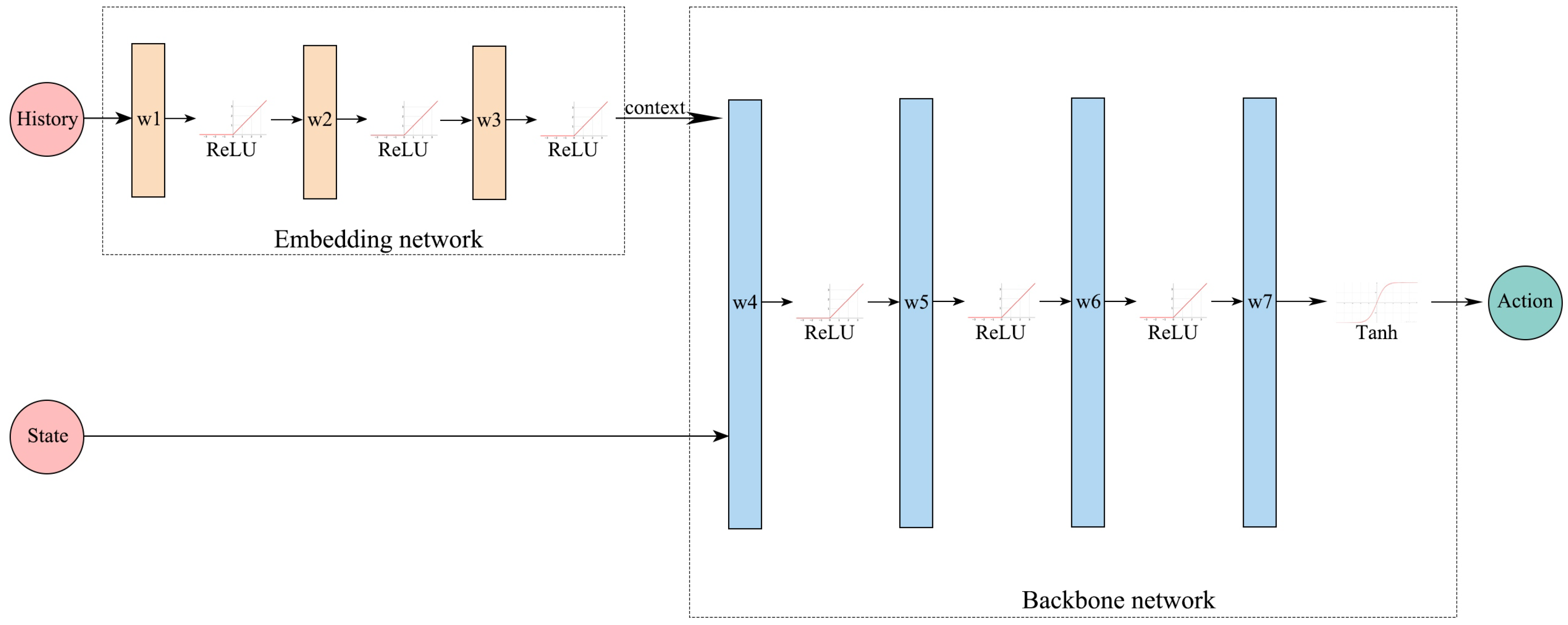
Previous reinforcement-learning-based controllers have typically only used the error vector at the current time as the state [27,28]. However, this approach limits the model’s ability to effectively infer the trend of environmental changes, resulting in excellent control performance only in the dynamic of training environments. Figure 4 shows that in this research, an embedding network is articulated at the input of the policy network to introduce context into the PPO model. This embedding network implicitly maps the motion trajectory sequences to contextual variables, thus including environmental information as part of the decision-making factors. The design has two main advantages: (1) Firstly, the context generated by the embedding network enables the policy to adapt to the environment online. (2) The training of the embedding network is integrated with the backbone network and the training process is more efficient compared to the alternating optimization approach [20].

The input of the policy contains two parts, the current state vector $state$ and the sequence of motion trajectory History, where $stat{e}_t$ is the state acquired by the AUV at the current moment t. Based on the task definition in Section 2.3, $state={[\Delta z,w,\Delta y,v]}^T$, $\Delta z$ and $\Delta y$ are the position error and velocity in the direction of $Heave$ and $Sway$, and w and v are the velocity in the direction of $Heave$ and $Sway$, respectively. Since the AUV model in this research is intrinsically stable in roll and pitch, the tracking control of roll and pitch can be neglected [29]. For a general torpedo body AUV, we propose to include angles in the state vector to describe the direction of the relative motion velocity. The motion track sequence $History$ consists of a sequence of states and actions in past moments: $Histor{y}_t=\left\{stat{e}_{t-N},u_{t-N}\dots stat{e}_{t-1},u_{t-1}\right\}$, N is the size of window. 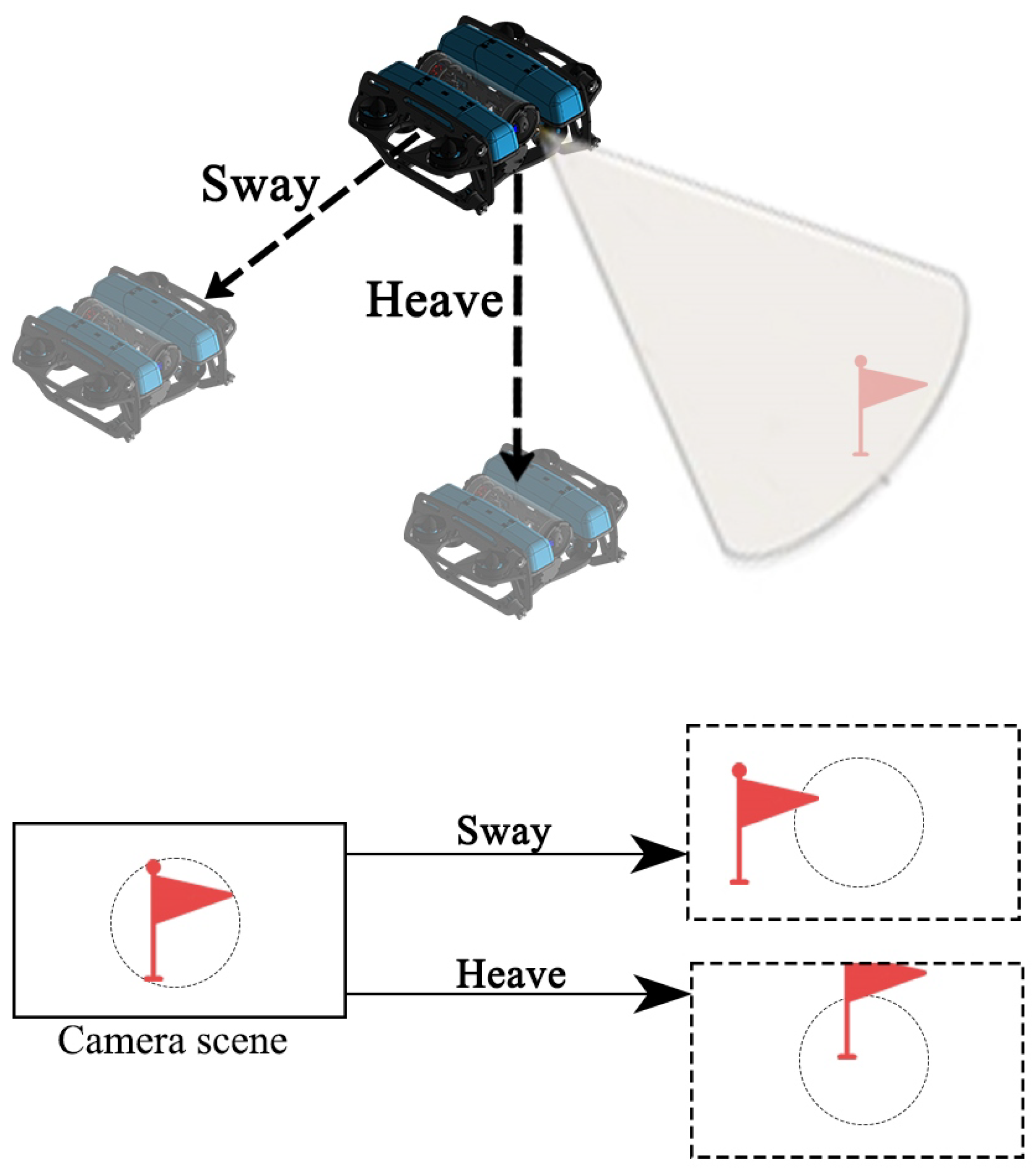The action u is defined as the propulsive force received in the sway direction and the heave direction: $u={[Y,Z]}^T$. The input dimension of the embedding network is $(4+2)\ast N$, while the input dimension of the policy network is $(4+2)\ast N+4$. The output dimension of the policy network is four, representing the mean and variance of the normal distributions of Y and Z. The critic network comprises three hidden layers that take the current state as input, and the output is a scalar value. Both the policy and the critic networks have 64 neurons in each hidden layer.

For the AUV target tracking task, not only the absolute error and response time of the system, but also the amount of overshooting and energy loss, should be considered. Therefore, the design reward function is mathematically expressed as follows:

$$r=-{\lambda }_1\sqrt{\Delta z^2+\Delta y^2}-\lambda \parallel a\parallel$$

(19)

The first term of the reward function is used to motivate the controller to reduce the error as quickly as possible to achieve a fast response to the position error. The second term motivates the controller to produce a smaller control amount to avoid overshooting, as well as to output limit values. ${\lambda }_1$ and ${\lambda }_2$ are scaling factors, which are used to adjust the weights of these two items.

For robot motion control, differences in dynamics resulting from modeling errors or external environmental forces can be represented as generalized forces $u^{\prime }=[Y^{\prime },Z^{\prime }]$ on the right-hand side of the dynamics equations. Valassakis et al. [30] proposed the use of generalized forces to describe modeling errors, which have a better profile and manipulability than randomizing environmental parameters and performed better in experiments. Therefore, this study created diverse training environments by sampling generalized forces. Specifically, before the start of each episode, $Y^{\prime }$ and $Z^{\prime }$ were sampled twice from a uniform distribution: $Y^{\prime }\sim U[-Y_{max,Y_{max}}]$, $Z^{\prime }\sim U[-Z_{max},Z_{max}]$, where $Y_{max}$ and $Z_{max}$ are the limit values of the sampling interval. As shown in Figure 5, the two sampled values were connected by a folded line to form a generalized force function that varied during one episode. The aim of this design was to simulate sudden and gradual changes in dynamics, as well as maintaining constant dynamics in the training environment.

3.2. Progressive Network Training Mechanism

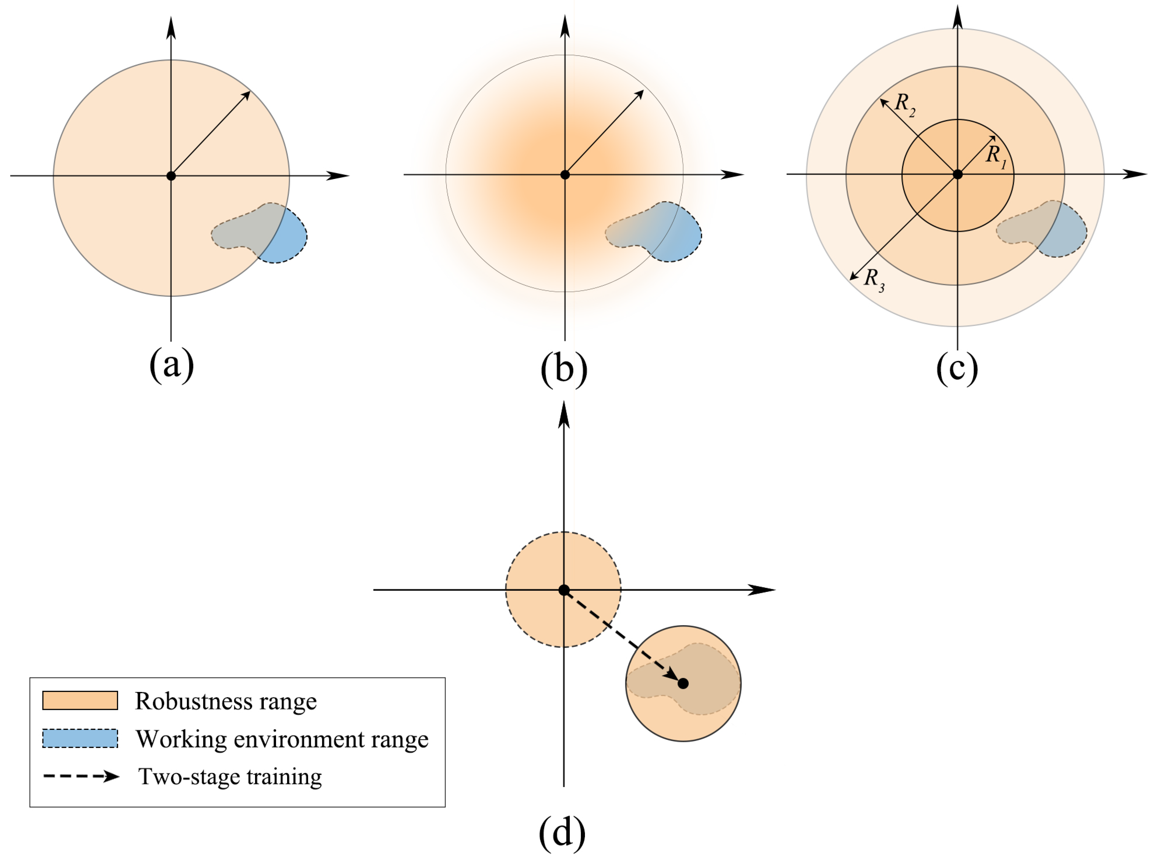
In order to build effective context mappings, i.e., to allow context information to characterize a wide variety of environments, it is first necessary to generate a large number of different training environments. A common approach is to use domain randomization, which generates environments randomly by sampling environmental parameters in a distribution [19]. Figure 6 shows a hyperplane representing the range of dynamics, with the origin at the center of the training environment’s dynamics and the orange region indicating the model’s range of robustness. The darker the color, the better the control performance of the model. In general, the dynamics of a real working environment is not fixed but varies within a certain range, so the dynamics range of the working environment is a region rather than a point in Figure 5. Figure 6a,b show the effect of sampling from uniform and normal distributions, respectively. Sampling from a normal distribution will make the model fully trained near the center of the dynamics, while the effect of a uniform distribution is more average. Figure 6c illustrates that a wider range of environments characterized by the context requires a larger training range to cover the unknown dynamics of the working environment, provided that the model size and the definition of the context remain the same. In order for the context mapping to cover the unknown dynamics of the working environment, a larger training range needs to be used, trading optimality for robustness.

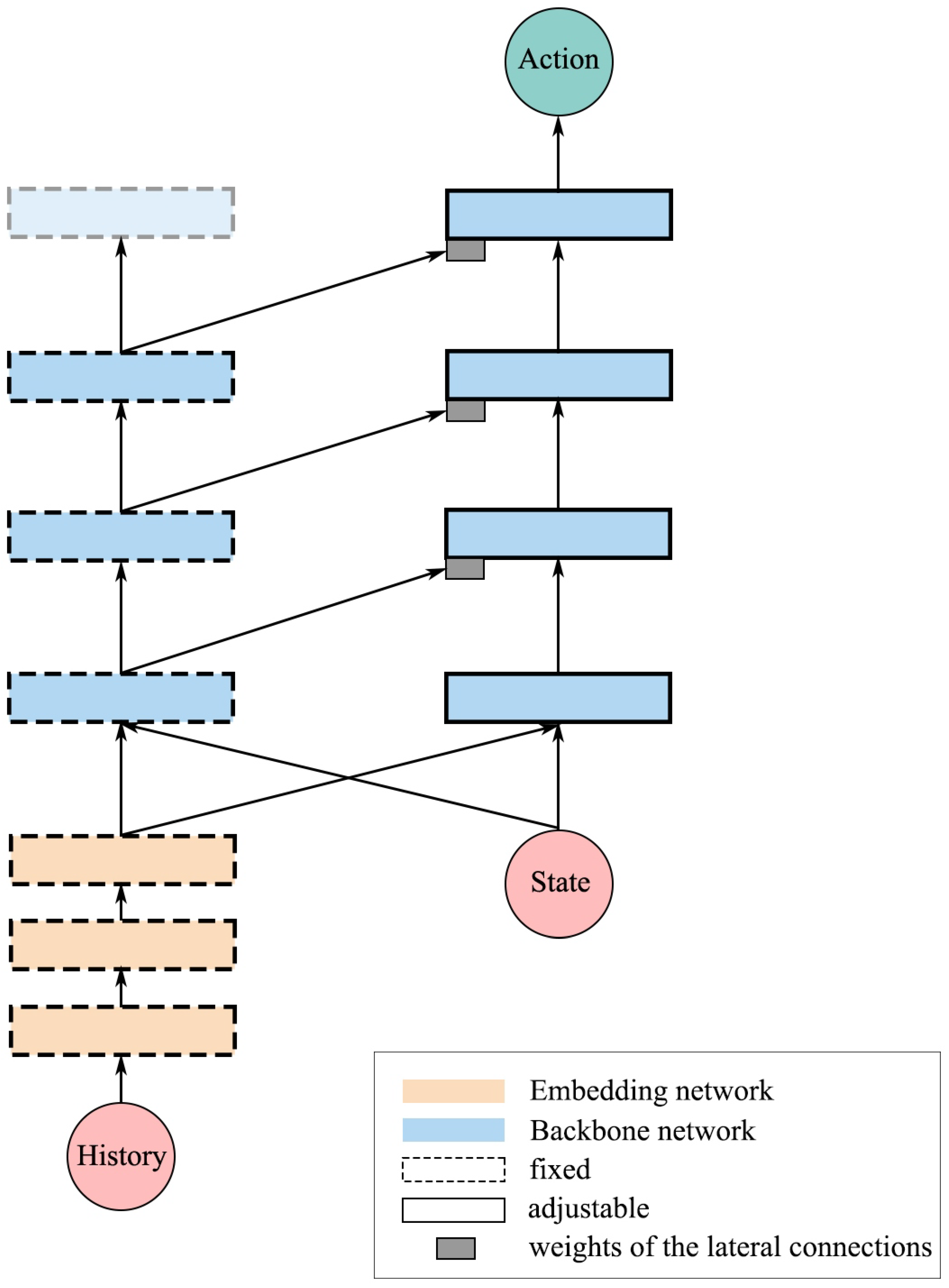
In order to solve the above problems, this study utilizes progressive neural networks to transfer the DRL model across various dynamics, as shown in Figure 7. The model comprises two network columns, with the left column representing the trained network and the right column representing the network that is to be optimized in the working environment. When trained in a working environment, the parameters of the left column are fixed, and the right column receives outputs from the network layers of the left column through lateral connections. These lateral connections enable the right column to extract useful features from the left column, which are adapted to the training environment, thus accelerating the learning process. As mentioned earlier, the work environment can vary within a certain range, making it impractical to add new columns whenever the environment changes. Therefore, the parameters of the embedding network are directly copied and fixed to enable the model to adapt online to small disturbances in the work environment. Figure 6d demonstrates that the two-stage training approach based on progressive network allows the model to transfer between very different dynamic environments, and the context-based policy architecture makes the model more robust to small perturbations.

3.3. Algorithm Process

A fast adaptive robust PPO (FARPPO) algorithm is proposed by combining a context-based policy architecture with a progressive network training mechanism. The training environment was created by uniformly sampling the generalized forces $Y^{\prime }$ and $Z^{\prime }$, a process known as domain randomization. We first initialized and fully trained a policy ${\pi }_{{\theta }_1}$, then initialized a policy ${\pi }_{{\theta }_2}$ and connected it laterally as shown in Figure 7. Finally, we trained FARPPO to convergence in the working environment. Algorithm 1 gives the main steps involved in the above process.

Algorithm 1: FARPPO for the target tracking of the AUV
	Input: initial critic network parameters $\varphi$; initial policy networks parameters ${\theta }_1$,${\theta }_2$; initial reply buffer B; the limit value of the sampling interval $Y_{max}^{\prime }$,$Z_{max}^{\prime }$
	Output: FARPPO policy network
1	for episode = 1:M do$\phantom{(}$$\phantom{(}$
2		Sample environment $env$ from $Y^{\prime }\sim U[-Y_{max}^{\prime },Y_{max}^{\prime }]$ and $Z^{\prime }\sim U[-Z_{max}^{\prime },Z_{max}^{\prime }]$
3		Collect transitions $(s,a,r,s^{\prime })$ from $env$ and store in B
4		if  B is full then
5			Compute GAE $A(s_t,a_t)$ based on the current Value function $V_{\varphi }$
6			for Reuse_times = 1:N do
7				Update policy network:${\theta }_1={\theta }_1+\alpha {\nabla }_{{\theta }_1}L\left({\theta }_1\right)$
8				Update critic network:$\varphi =\varphi +\beta {\nabla }_{\varphi }MSE\text{\_}Loss(V_{\varphi }\left(s_t\right),r_t+\gamma V_{\varphi }\left(s^{\prime }\right))$
9			end
10			clear B
11		end
12	end
13	Connect the two policy networks laterally as FARPPO according to Figure 7
14	Frozen ${\theta }_1$, initializes $\varphi$, clear B
15	Deploy FARPPO to the work environment $Env$
16	while not converged do
17		Collect transitions $(s,a,r,s^{\prime })$ from $Env$ and store in B
18		if B is full then
19			Compute GAE $A(s_t,a_t)$ based on the current Value function $V_{\varphi }$
20			for Reuse_times = 1:N do
21				Update policy network:${\theta }_2={\theta }_2+\alpha {\nabla }_{{\theta }_2}L\left({\theta }_2\right)$
22				Update critic network:$\varphi =\varphi +\beta {\nabla }_{\varphi }MSE\text{\_}Loss(V_{\varphi }\left(s_t\right),r_t+\gamma V_{\varphi }\left(s^{\prime }\right))$
23			end
24		end
25	end
26	return

3.4. Computational Complexity Analysis

We analyzed the time computational complexity of the FARPPO algorithm using big O notation denoted by $O[·]$.

Initialize the network parameters, such that the number of each network parameter is N. The time complexity required for initialization is $O\left[\mathrm{N}\right]$. In the main loop, the key steps include environment sampling, data collection and storage, updating the policy and critic network, and emptying the cache area, such that the number of iterations of the main loop is M and the state dimension is S. The time complexity required for a single main loop is $O\left[1\right]+O\left[1\right]+O\left[\mathrm{S}·\mathrm{N}\right]+O\left[\mathrm{N}·\mathrm{S}\right]+O\left[\mathrm{N}·\mathrm{S}\right]+O\left[1\right]$, this can be simplified as $O\left[\mathrm{N}·\mathrm{S}\right]$, so the overall time complexity is $O\left[{\sum }_{i=1}^{\mathrm{M}}\mathrm{N}·\mathrm{S}\right]$; the time complexity of the policy network combination and parameter freezing part is $O\left[\mathrm{N}\right]$, in the training phase, the main loop is trained continuously until convergence, each time. The key steps include the environmental interaction and the experience of the reuse and updating, so that the convergence and the number of iterations required is T, and then the time complexity is $O\left[{\sum }_{i=1}^{\mathrm{T}}\mathrm{N}·\mathrm{S}\right]$. Synthesizing the above analysis, the total time complexity of the whole algorithm is $O\left[\mathrm{N}\right]+O\left[{\sum }_{i=1}^{\mathrm{M}}\mathrm{N}·\mathrm{S}\right]+O\left[\mathrm{N}\right]+O\left[{\sum }_{i=1}^{\mathrm{T}}\mathrm{N}·\mathrm{S}\right]$, This can be simplified as $O\left[{\sum }_{i=1}^{\mathrm{M}+\mathrm{T}}\mathrm{N}·\mathrm{S}\right]$. where N: number of network parameters; S: dimensions of the state space; M: number of iterations in training phase 1; T: number of iterations required for convergence in the deployment phase.

The space complexity is mainly related to the number of network parameters and the size of the experience playback buffer, and when the number of network parameters in the assumption above is N, then the complexity is $O\left[\mathrm{N}\right]$. Let the buffer size be set to B, assuming that the storage of state, action, reward, and other information requires space $O[\mathrm{S}+\mathrm{A}+1]$, where A is the dimension of the action space, so the space complexity is $O[\mathrm{B}·(\mathrm{S}+\mathrm{A}+1\left)\right]$. The overall space complexity is $O\left[\mathrm{N}\right]+O[\mathrm{B}·(\mathrm{S}+\mathrm{A}+1\left)\right]=O[\mathrm{N}+\mathrm{B}·(\mathrm{S}+\mathrm{A}+1\left)\right]$. This indicates that the proposed algorithm is capable of being implemented in real-time operations.

The FARPPO algorithm involves multiple policy and value network update operations, especially internal nested loops, which increase the stability of the policy and the accuracy of the decision but also imply a high computational load. In order to prevent a combinatorial explosion from causing difficulties in solving the problem, we recommend that the number of state network parameters (N) be kept within the thousand-digit range, and that the number of state-space dimensions (S), the number of iterations in the training phase1 (M), and the number of iterations required for convergence in the deployment phase (T) be kept within the hundred-digit range.

4. Experiments

4.1. Experiment Settings

The computing platform used in this study was an Intel(R) Core(TM) i7-6700H@2.60GHz and NVIDIA GeForce GTX 1060 (Intel, Santa Clara, CA, USA). The OS was Ubuntu18.04. The numerical simulation environment, implemented in Python 3.7.11 using numpy, used the fourth-order Rung–Kutta method to solve a differential equation at each time step with a time step size of 0.1 s. The neural network was implemented in Python using pytorch, and parameter settings related to the algorithm in this paper are shown in

Table 2. Parameters of algorithm.

Parameters	Value
Discount factor $\gamma$	0.98
Clip epsilon $\epsilon$	0.2
Batch size	64
Max train episode M	500
Episode max step	100
Limit value of sampling $Y_{max}$	70
Limit value of sampling $Z_{max}$	50
Fixed time node $T_1$	30
Fixed time node $T_2$	60
Reuse_times N	8
Scale factor ${\lambda }_1$	1
Scale factor ${\lambda }_2$	0.01
Learning rate of the policy network $\alpha$	0.0002
Learning rate of the critic network $\beta$	0.0002

.

Discount factor ($\gamma$): The discount factor is used to weigh immediate rewards against future rewards in reinforcement learning. A value close to 1 means that future rewards are almost as important as immediate rewards, while a lower value means that immediate rewards are valued more highly. A value of 0.98 is a common choice, which indicates that future rewards are valued slightly less than immediate rewards. Clip epsilon ($\epsilon$): $\epsilon$ determines the balance between exploration (trying new behaviors) and exploitation (using the best known behaviors). $\epsilon =0.2$ ensures that the exploration behavior is within a certain range; Batch size: Batch size determines the number of samples used in each training iteration. Larger batch sizes provide more stable gradient estimates, but can lead to memory problems and longer training times; 64 is a common compromise. Max train episode (M): The maximum number of training episodes determines how many full learning cycles the algorithm will run. This value needs to be large enough for the algorithm to learn and adapt to the environment. Episode max step: The maximum number of steps per episode limits the length of a single episode, which helps prevent infinite loops and ensures that the algorithm can finish learning in a reasonable amount of time. Limit value for sampling ($Y_{max},Z_{max}$): These parameters are used to limit the maximum value of the variables in the sampling process, to prevent them from becoming too large, which would affect the stability and performance of the algorithm. Fixed time node ($T_1,T_2$): These fixed time nodes are used for evaluating or adjusting the behavior of the algorithm at a specific point in time, during the strategy evaluation phase in reinforcement learning. Reuse times (N): This parameter refers to the number of times the data are reused, where a higher number of reuse times improves efficiency. Scale factor (${\lambda }_1,{\lambda }_2$): The scale factor is used to adjust the weights of the components in the algorithm. Learning rate of the policy network ($\alpha$): The learning rate of the policy network determines how often the network weights are updated in each training iteration. A lower learning rate leads to a more stable training process. Learning rate of the critic network ($\beta$): Similarly to the policy network, the learning rate of the critic network determines the frequency of updating the weights. In many algorithms, these two learning rates are set to be the same, to maintain a balance between the two.

4.2. Robustness Simulation Experiments

In order to verify the robustness of FARPPO to environmental disturbances, we tracked the depth step response using FARPPO and the original PPO-Clip, where PPO-Clip did not include an embedding network in the actor network, its input was the current state, and it was trained in an environment without generalized forces.

Currents and undercurrents are two types of environmental disturbances to which AUVs are often subjected when operating in underwater environments. Currents change very slowly and can be regarded as stable constant disturbances; in deep water, the effect of currents on the vertical plane of motion of an AUV is weak, and the main disturbances suffered by the AUV are transient disturbances from undercurrents. In the experiment, the AUV moved from an initial position (0, 0) to a target depth of 5 m in 100 s and moved in the Y-axis to a target point with coordinates of 3 m. We set up three kinds of disturbances in the $Heave$ axis, which included constant values, step signals, and sine waves.

In Figure 8, we give the step response of FARPPO and PPO-Clip in an environment with interference. The first, second, and third rows of pictures show the step response of the AUV under constant force interference, step force interference, and sinusoidal force interference. As a reference, we give the control performance indicators of each algorithm in depth step response in

Table 3. Control performance indicators for step response.

Disturbance	Indicators	FARPPO	PPO
constant	steady-state error (m)	0.03	0.8
	overshoot (%)	3.3	0
	adjustment time (s)	23.2	17.6
step	steady-state error (m)	0	0.5
	overshoot (%)	2.0	4.6
	adjustment time (s)	10.7	12.7
sinusoidal	steady-state error (m)	0.05	0.6
	overshoot (%)	5.4	54.5
	adjustment time (s)	31.6	63.3

. The adjustment time is the time required for the controlled object to reach the steady-state, the overshoot indicates the ratio of the maximum offset to the steady-state depth, and the steady-state error indicates the difference between the desired depth and the actual depth.

As can be seen from Figure 8 and Table 3, the step response of the PPO-Clip algorithm showed a significant steady state error when there was constant value interference in the environment. This phenomenon is expected when thinking from a controller design perspective. This is because when designing a DRL controller in the conventional way, the inputs to the controller are the error and state at the current moment and the outputs are the level of actuator action (e.g., propeller speed) of the AUV. In this case, the DRL model was adapted during training to achieve precise control in the dynamics of the training environment. When a constant force was present in the environment, the DRL model was still controlled in terms of the characteristics of the training environment dynamics, and when the relative error between the AUV and the desired depth reached a specific value, the amount of action output from the DRL model canceled out the constant force disturbance, and this specific value was the steady-state error that occurred in the DRL model. This again explains the response of PPO-Clip in the presence of a step disturbance in the environment. In contrast, FARPPO had almost no steady-state error in the presence of a step disturbance and could maintain a much smaller overshoot and faster response. When a step disturbance was present in the environment, the tracking curve of FARPPO showed only a small float and adapted quickly to the new environment. When continuously varying sinusoidal disturbing forces were present in the environment, the PPO-Clip was no longer able to complete the tracking control task, while the FARPPO maintained good control performance.

4.3. Adaptability Simulation Experiments

In order to verify the ability of FARPPO to quickly adapt to new working environments, we set up two control algorithms: Two-stage and $Zero$. The policy network of both algorithms followed the design of Figure 4. Two-stage was first trained in the simulation environment and then deployed to a new working environment for two-stage training, but it did not use a progressive network-based training mechanism. $Zero$ started training directly in the working environment.

An AUV may encounter certain scenarios where the mass changes while working, such as water sample collection and dropping target missions, or with an AUV in the deep sea where the mass changes due to pressure effects. Control methods based on accurate models may no longer be effective in these cases, due to the unknown mass change. In addition, according to Equation (5), compared with the generalized force, a mass change leads to a change of several term coefficients, which makes the dynamical model more complicated. Therefore, we chose a representative task with mass changes to test the adaptability of the algorithm. In the simulation, we reduced the mass of the AUV by 10% (12.15 (kg)) and 25% (10.13 (kg)), and then increased it by 10% (14.85 (kg)) and 25% (16.87 (kg)), respectively, while all the other parameters remained constant.

As network training involves randomness, we trained each set of algorithms 10 times with different random seeds. The reward curves in Figure 9 show that the Two-stage algorithm took longer to tune in the new dynamics when there was a change in mass. When the difference in dynamics was significant (at 25% change in mass), the Two-stage model required more data to converge than the $Zero$ model. This shows that the direction of parameter optimization for a DRL agent in environments with significant differences in dynamics may vary considerably. The training speed of a two-stage algorithm may be slower than the method of initializing and training the parameters directly in the new environment. In contrast, FARPPO exhibited the fastest training speed in all environments, and the training process was notably stable, providing evidence that the training mechanism proposed in this study was effective. The lateral connections enabled the policy network to leverage useful features extracted from the training environments, thereby accelerating the learning process.

An experiment was conducted on the relationship between adaptation and robustness. In this experiment, the sampling parameter for the training environment was the mass of the AUV, as shown in Figure 10. Two sets of control experiments were conducted, where Model A and Model B randomly sampled the mass within the ranges of $[0.9mass,1.1mass]$ and $[0.8mass,1.2mass]$ during the training period. The mass was subsequently sampled in both training ranges, and two masses, M and N, were randomly selected as working environments. The study proposed a training mechanism to transfer A to a dynamic environment centered on 0.8 mass. The working environment Q was selected for a comparison of the depth step response between the two models at points M, N, and Q. Figure 10 shows that both M and N fell within the training range of models A and B. Although the step responses of both models were satisfactory, the response curves of model B, which had a larger training range, exhibited slightly more fluctuations. Point Q fell outside the training range of model B, and the response curves of model B at point Q no longer met the general control requirements. This suggests that the policy’s robustness, gained through the context, may have fallen outside the training range. The response curve of model A remained satisfactory after migration, fully demonstrating the effectiveness of FARPPO in the process.

4.4. Simulation Result Analysis

Figure 8 shows that the control performance of the conventional DRL model decreased significantly when the environmental dynamics changed. From a controller design perspective, a DRL controller without context is equivalent to a PID controller without integration and differentiation, except that in DRL, the proportional element “P” in PID is a nonlinear mapping composed of a neural network. While neural networks have shown impressive performance in certain tasks, they cannot fully replace the role of integral and differential elements. In Figure 8, the control performance of FARPPO is significantly better than that of PPO-Clip, because the embedding network provided the policy with the ability to resist disturbances within a certain dynamic range by mapping the motion trajectory data onto more complex contextual information than integration and differentiation.

Figure 9 shows that the FARPPO algorithm outperformed the two-stage training method in terms of training speed and stability. The field of transfer learning faces a problem known as ‘catastrophic forgetting’, which refers to a model’s inability to process previously learned tasks after adapting to a new one. The optimization of parameters may not be similar for similar tasks, and parameters trained on different dynamics may not be suitable as initialization parameters. However, in practice, few AUV researchers have directly collected training data using a real AUV, and most still use the two-stage training method. Therefore, the training architecture of FARPPO provides a new concept for future work. Thanks to its lateral connections, FARPPO can extract useful information from the previous dynamical context. This makes the training process more efficient, with faster convergence of the reward curves and less variance. Figure 10 illustrates that the robustness of the policy obtained from the context was related to the training range, which could be migrated using the training method based on a progressive network. This further confirmed the effectiveness of the context-based policy architecture and the progressive network training mechanism. It can be seen that the FARPPO algorithm, through its advanced architecture and training mechanism, demonstrated significant advantages in both control performance and training efficiency, especially when dealing with changes and disturbances in environmental dynamics. Meanwhile, the asymptotic network and context-based policy architecture provide effective solutions to address challenges in transfer learning.

4.5. Depth Control Experiment

4.5.1. Experimental Platform Design

The experimental platform chosen for this paper was FindROV C20H (Intel Corporation, Santa Clara, CA, USA), a small high-performance remotely operated underwater robot. Compared with BlueROV Heavy, the control compartment of the FindROV C20H used in this study is made of more pressure-resistant materials, and its weight is increased by 0.5 kg, while other aspects are the same as the BlueROV Heavy. In terms of thruster configuration, it is equipped with eight T200 thrusters (Blue Robotics, CA, USA), to produce stabilized control in six degrees of freedom through vector propulsion, as shown in Figure 11 and Figure 12. For vision, the front of the robot is equipped with a high-definition (1080p, 30 fps) wide-angle low-light camera and two dimmable lumen lamps providing 6000 lumens of brightness, to provide stable visual information for the vision-guided-control-based approach. The robot is designed with an open frame to carry electronics and battery housings, thrusters, buoyant foam, and ballast. The design is rugged and scalable, offering the possibility of retrofitting the AUV model.

The hardware connection of the experimental platform is shown in Figure 13. The connection accessories contained three items: a communication cable, power carrier, and PC computer. The PC computer could obtain sensor information and send control signals through the ground control software QGC (Q Ground Control) (https://searobotix.com/learn/qgroundcontrol-guide/ accessed on 21 November 2024), and a PC computer was connected to the power carrier through a USB interface, which transmitted the communication signals to the single-board computer inside the robot through an 8-core cable Raspberry Pi (Aohai, Hangzhou, China).

In this study, the experimental platform was transformed into an autonomous underwater robot by extending a waterproof central control compartment, as shown in Figure 14. First of all, for the sake of shooting experimental videos and safety considerations, the maximum depth of the real voyage experiment was about 1 m underwater, so the IP68 grade waterproof box (LEPPU, Wenzhou, China) was sufficient to meet the waterproof requirements. There were three objects in the waterproof box: the main Nvidia Jetson AGX Orin control computer (Intel, Santa Clara, CA, USA), the 12 V DC power (Delipow, Shenzhen, China) supply to power it, and the Fathom-X power carrier (Aohai, Hangzhou, China). An Nvidia Jetson AGX Orin was chosen as the host computer to replace the PC for the deep reinforcement learning controller designed in this study, which requires the use of neural networks, as well as for running the target detection model in the subsequent visual guidance experiments. Its arithmetic power reaches about 200 TOPS, which is equivalent to almost 8–10 times the current mainstream devices and can meet the demand of running deep reinforcement learning models and target detection models at the same time. Second, a waterproof 8-core cable with a shorter length was used instead of the original communication cable, and a watertight cable waterproof plug and a Lingke LP-16 type female connector (Aohai, Hangzhou, China) were soldered at each end to connect the power carrier and the robot. The communication cable passed through a perforation on one side of the watertight compartment, which was made watertight using a PG9 watertight connector (Aohai, Hangzhou, China) and a rubber gasket. After testing, the waterproof performance of the waterproof compartment met the experimental requirements.

4.5.2. Experiment Settings

In order to verify the performance of the algorithms proposed in this paper in a real environment, fixed depth control experiments were conducted using the above experimental platform. Three groups of algorithms were set up in the experiment: the proposed method, the PPO, and the PID algorithm. The proposed method was the algorithm proposed in this paper, which was first trained in the environment with interference, as described in Section 3 of this paper, and then bipartite training was carried out in the real environment based on the asymptotic network, with the process as described in Section 3.2 of this paper. The PPO is a traditional reinforcement learning controller, where history is not introduced in the state design, and only the current position error and velocity were used as inputs and trained directly in the real environment.

4.5.3. Experimental Results and Analysis

In the fixed depth experiment, the initial depth of the AUV was 0 m (water surface) and the target depth was 0.5 m. To test the robustness of each controller to external disturbances, we placed a dumbbell piece with a weight of 5 kg on the AUV as a step disturbance 5 s after the start of the experiment, and the experimental procedure was as shown in Figure 15. The depth response curves of each controller are shown in Figure 16, Figure 17 and Figure 18.

In this case, the proportional, integral, and differential coefficients of the PID controller were set to 130, 1.5, and 0, respectively, after optimization by artificial tuning. As can be seen from the figure, the curve of the PID controller was smoother and the amount of overshooting was smaller before the appearance of perturbation, while the quality of the control was better compared to that of the DRL-based controller. The PPO algorithm used in this study was a stochastic strategy, where the network output a normal distribution and sampled action values from it, thus introducing instability, so the AUV had some fluctuations in the depth curve after reaching the target value.

From the second half of the curve, it can be seen that the AUV sunk to the bottom rapidly after a weight was placed on the top, because the PPO controller could not adapt to the environmental changes. The output of the PID controller reached a steady state value before the weight was placed, and after the weight was placed, the integrating link resulted in the output of the controller increasing continuously, and the depth position of the AUV gradually tended toward the target value. The target tracking task often requires a certain response time, so the time set for this experiment was shorter, and the PID controller needed a longer experimental time to accumulate the amount of error needed to correct the error. In contrast, the algorithm proposed in this paper quickly adapted to the environment after fluctuations and accomplished the depth tracking task under weight-bearing conditions.

This experiment demonstrated that the improved context-based algorithm could enhance the robustness of the reinforcement learning controller. Although the PPO algorithm trained in the real environment showed better control performance without perturbation, it had difficultly in accomplishing the control task when the environment changed or perturbation occurred. Compared with the linear control law of the PID controller, the algorithm proposed in this paper maps the historical data into contextual information characterizing the environmental properties through neural networks in each control cycle, which is a more powerful way of characterizing the environmental properties, giving the DRL controller the ability to adapt to the environment online.

In the training process in the pool, the target was fixed to the wall of the pool, and 300 rounds of training were sequentially performed for the forward, lateral, and depth position controllers. Before the start of each round, the AUV position was manually adjusted so that the absolute value of the forward and lateral initial position error was less than 1.2 m. Compared with the fixed initial position, the randomized initial position allowed the AUV to explore the state space more fully. Since the AUV had micro-positive buoyancy, the AUV automatically floated to the water surface at the beginning of each round, so the initial depth error was 1.2 m. The input–output structure of each controller also followed the setup in Section 3 of this paper, with the proposed method taking the history of motion data, current position error, and velocity as inputs; the PPO taking the current position error and velocity as inputs; and the PID taking the current position error and velocity as inputs; all controllers taking the current position error as input; and the PID taking the current position error as inputs. The outputs of each controller were the propulsive force in the forward, lateral, and depth directions, which were converted to the rotational speed of each thruster through the robot’s built-in thrust distribution system.

According to Figure 19, in the training process of the forward position controller, the algorithm proposed in this paper converged in around 150 rounds, while the PPO converged in around 200 rounds, and the training speed of the algorithm proposed in this paper was about 1.3 times that of the PPO algorithm; from Figure 20, in the training process of the lateral position controller, the algorithm proposed in this paper converged in around 150 rounds, while the PPO converged in around 250 rounds. It can be seen from Figure 21 that, in the training process of the lateral position controller, the proposed algorithm converged in about 150 rounds, while the PPO converged in 250 rounds, the training speed of the proposed algorithm was about 1.7 times that of the PPO algorithm, and the fluctuation of the rewards of the proposed method was significantly smaller than that of the PPO, which fully proves that the bipartite training mechanism based on the gradual network proposed in this paper can effectively improve the training speed and the training stability of AUVs in real underwater environments. As can be seen from Figure 21, there was no significant difference between the training speed of the algorithm proposed in this paper and the PPO during the training process of the depth position controller. We suggest that this was because the hardware modification (placing a waterproof box above the AUV) had a large impact on the depth-direction motion, and when the AUV dived or floated up near the water surface at high speed, the splashing waves and bubbles on the water surface caused the vision system to fail to recognize the target, and there was a delay in the acquisition of the sub-states by the AUV, which resulted in the reward error.

In summary, we can conclude that the FARPPO algorithm, through its advanced contextual processing capability and progressive network training mechanism, demonstrated significant advantages in control performance, training speed, and environmental adaptability, providing an effective solution for the control of autonomous underwater vehicles such as AUVs.

4.6. Visual Guidance Tracking Experiment

4.6.1. Experiment Settings

Based on the above research results, this study combined the target detection technology with the proposed algorithm to build a visually guided AUV tracking control system. In terms of target detection, YOLOv8 [31] was chosen as the target detection model, and it was compared with YOLOv10 in this study.

YOLOv8 provides several sets of pre-trained parameters, so that users can select model parameters where the accuracy and computing speed meet their requirements. In this experiment, the official pre-trained model parameters of YOLOv8s were used to balance the computing speed and accuracy. During the experiment, the real-time image of the camera was detected, and the results are shown in Figure 22.

In the experiment, we used a cup as the target (i.e., the cup in the figure), fixed it at the end of a long pole, and manipulated its movement by hand. The detection result of the YOLOv8 model could directly output the coordinates of the upper left corner of the target (x1, y1), as well as the lower right corner of the target (x2, y2), and the origin of the coordinates was in the top-left corner of the screen, the units of which were pixels. At this time, the center coordinates of the target were as follows:

$$\left(x_c,y_c\right)=\left({\displaystyle \frac{x2+x1}{2}},{\displaystyle \frac{y2+y1}{2}}\right)$$

(20)

The camera screen specification was 1080p, so the center of the target was offset from the center of the screen:

$$\left(x_e,y_e\right)=\left(540-x_c,960-y_c\right)$$

(21)

The area of the target was

$$s=\left(x2-x1\right)\ast \left(y2-y1\right)$$

(22)

It should be noted that the camera viewing angle corresponded to the vertical plane of the AUV, so the image offset $x_e$ corresponded to the displacement of the AUV in the sway direction, $y_e$ corresponded to the displacement of the AUV in the heave direction, and the image area corresponded to the displacement of the AUV in the surge direction. According to the size of the target and the specification of the camera screen, the conversion relationship between the target image offset and the AUV position error was obtained through experimental calibration:

$$\Delta x=\left(\sqrt{{\displaystyle \frac{s}{10,800}}}-1\right)\ast 0.6$$

(23)

$$\Delta y=(1+{\displaystyle \frac{\Delta x}{0.6}})\ast {\displaystyle \frac{3}{640}}\ast x_e$$

(24)

$$\Delta z=(1+{\displaystyle \frac{\Delta x}{0.6}})\ast {\displaystyle \frac{1}{2160}}\ast y_e$$

(25)

4.6.2. Data Transmission Link

During the operation of the AUV, the IP address of the host computer was set to make an Ethernet connection between it and the Raspberry Pi via USB, and a program was written based on the Pymavlink library to read video streams on the 5600 UDP port, or to read sensor data and send control commands over the 14,550 UDP port. Inside the master computer, after reading the real-time image from the camera through the 5600 UDP port, the visual detection module (YOLOv8 YOLOv10 model) was used to detect and convert the result into tracking position error. The deep reinforcement learning-based controller received the input from the target detection model and output the control quantity, which was converted into Pymavlink motor drive commands and sent to the controller through the 14,550 UDP port. The deep reinforcement learning-based controller received inputs from the target detection model and output the control quantities, which were converted into Pymavlink motor drive commands and sent to the Raspberry Pi via the UDP port 14,550. The above programs for data communication, target detection algorithm, and control algorithm were all implemented based in Python. The main Python program was opened in the terminal by writing a shell file to track the cup category targets in the camera image. The AUV control system was set to run automatically after the control computer was powered on by setting the shell file as power-on self-start.

4.6.3. Experimental Results and Analysis

According to the basic assumptions in Section 2.2 of this paper, the position tracking controllers for the surge, sway, and heave directions were set up based on the YOLOv8 and YOLOv10 algorithms. The target was fixed in the rigid linkage and manually manipulated, and the same trajectory and speed of the target were ensured by pre-marking the trajectory and synchronized timing in the experimental site. In the surge direction, the target started to move faster at 3 s; in the sway direction, the target moved continuously and slowly; and in the heave direction, the target changed state at a high speed at 2 and 5 s, respectively. The error curves during the experiment are shown in Figure 23, Figure 24 and Figure 25.

As can be seen from Figure 23, when the target moved slowly, the maximum position error of the three control methods based on the YOLOv8 and YOLOv10 algorithms in the tracking process did not exceed 10 cm, maintaining a better position tracking effect, and the overall effect of using the v8 and v10 input algorithms was similar. When the target moved faster, the control curves of PPO and PID in Figure 24 began to show larger errors, and it is obvious that the peak error when using YOLOv10 as input was significantly larger than that when using YOLOv8 as input. When the error was sufficiently large, the control quantities of the two algorithms of the PPO and PID resulted in the same moving speed of the target and the error returned to zero after the target finished moving. In this paper, the proposed algorithm always had less error in the tracking process. As shown in Figure 25, when the target moved at a high speed, based on the YOLOv8 and YOLOv10 algorithms, the PPO algorithm responded more slowly and lost the target during the tracking process, and it failed to complete the tracking task. Compared with PID, the algorithm proposed in this paper had a faster response, smaller error in the tracking process, and higher tracking accuracy. In summary, we believe that the algorithm proposed in this paper is superior, and using YOLOv8 and YOLOv10 as the inputs of the control had a similar effect on the system. So we can conclude that YOLOv8 was sufficient for this study.

In order to minimize the influence of manual operation randomness on the experimental results, each group of algorithms conducted 10 experiments to calculate the mean and standard deviation of the absolute value of tracking error of each group of algorithms, as shown in

Table 4. Target tracking performance indicators.

Algorithms	Controllers	Average Value	Absolute Value
Proposed method	forward direction	0.09	0.07
	sideway direction	0.08	0.05
	depths	0.10	0.07
PPO	forward direction	0.20	0.14
	sideway direction	0.11	0.08
	depths	0.27	0.18
PID	forward direction	0.15	0.10
	sideway direction	0.13	0.06
	depths	0.16	0.11

.

Based on the experimental results, it can be concluded that, due to the existence of many uncertainties in real underwater environments, the reinforcement learning controller designed using traditional methods had too large a dynamics gap to accomplish the control task; the PID controller demonstrated better tracking than the PPO by rectifying the parameters of the linear control law. However, for nonlinear AUV systems, the linear control law is often not optimal.

Table 5. Comparison of FARPPO, PPO-Clip, and PID performance metrics.

Algorithms	Robustness Simulation Experiments	Depth Control Experiment	Visual Guidance Tracking Experiment
Proposed method	Smaller steady-state errors occurred	Quickly completed depth tracking tasks	Quickly complete depth tracking tasks
PPO	Significant steady-state error occurred	Unable to complete depth tracking tasks	Tracking tasks were accomplished, but there was a high level of overshooting
PID		Longer time required to complete tracking tasks	Slow completion of tracking tasks

shows a comparison of the performance of the three algorithms in the experiments of this paper; the improved algorithm proposed in this study could effectively improve the control quality of the reinforcement learning controller by interacting with the real environments and explicitly optimizing the parameters of the strategy, which resulted in a higher tracking accuracy than that of the PID controller; the two-stage training mechanism based on the asymptotic network effectively improved the training speed and stability of the reinforcement learning controller in real underwater environments, which overcame the difficulty of training the reinforcement learning controller on real AUVs to a certain extent. The controller effectively improved the training speed and stability of the reinforcement learning controller in the real underwater environment, and to a certain extent, it overcame the difficulty of training a controller on a real AUV, which has significance for practical engineering applications.

Table 5 shows a comparison of the performance of the three algorithms in the experiments of this paper.

5. Conclusions

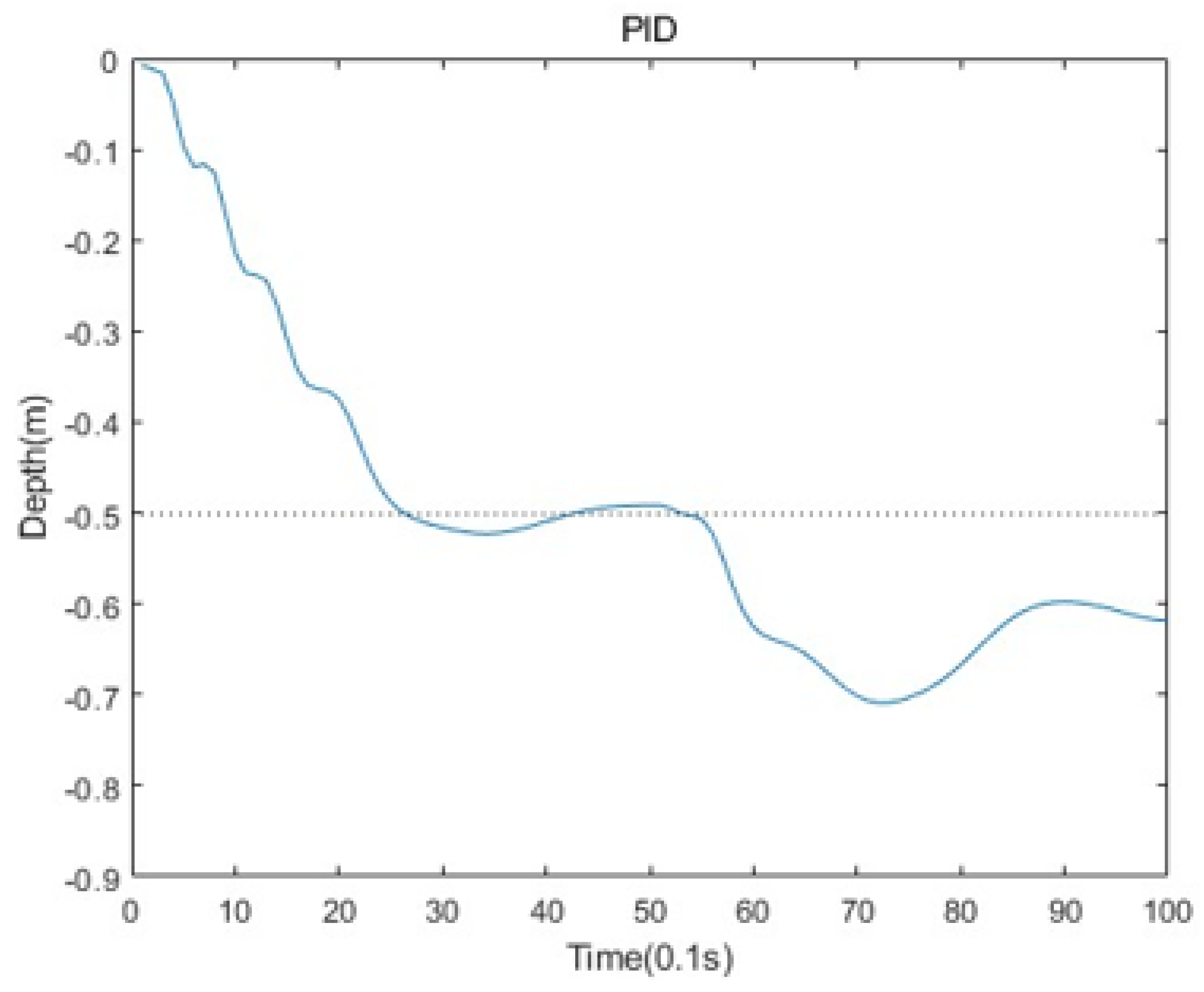
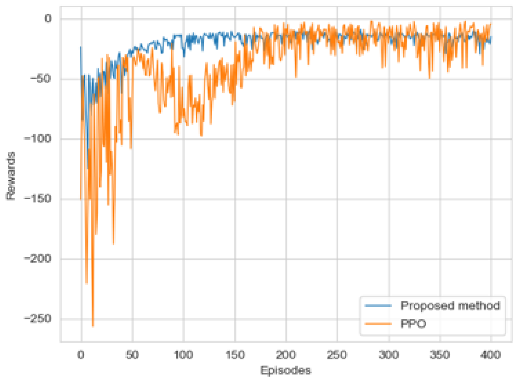
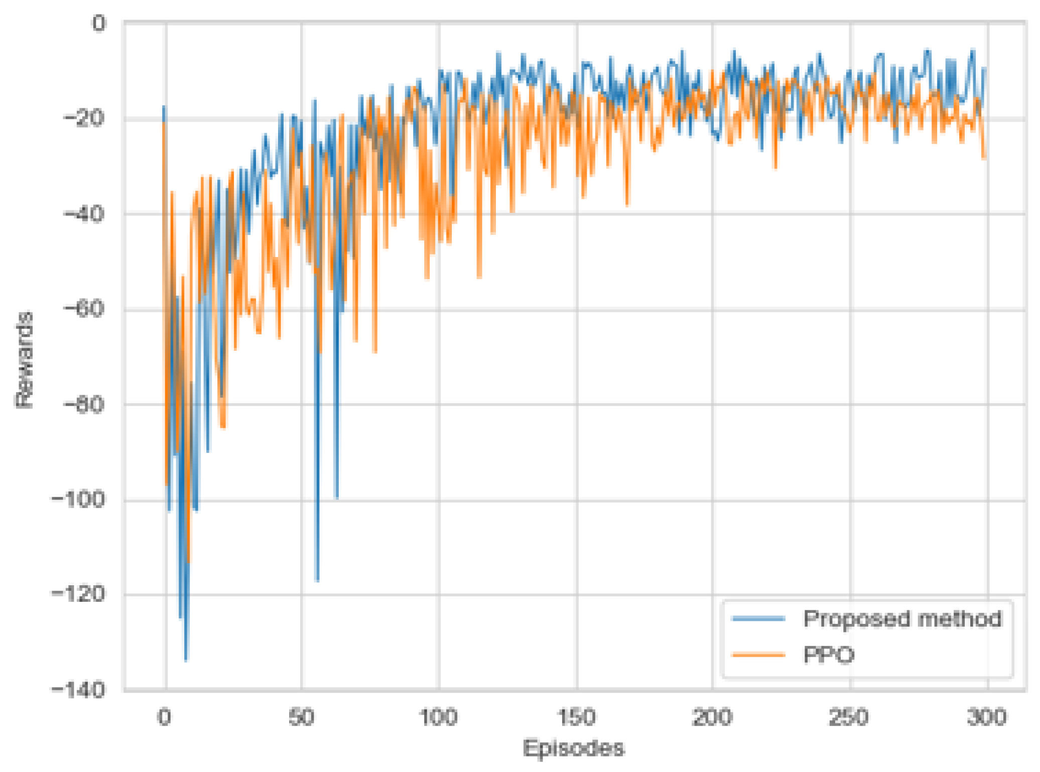
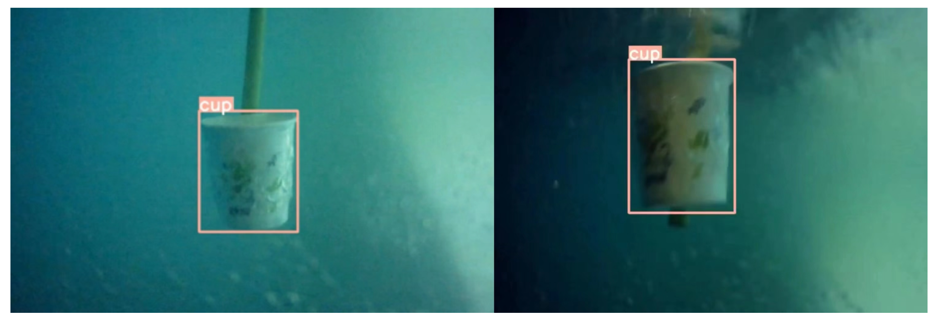
This paper proposed a new algorithm, FARPPO, for controlling AUVs. Firstly, we established a mathematical model of the AUV motion system and describd the basic task settings. Then, we designed FARPPO, improving the network structure and training method to achieve the integration of the advantages of the two methods. The visually guided tracking control experiments were carried out based on YOLOv8 and YOLOv10, and it was found that the input message from YOLO had little effect on the FARPPO. Compared with the traditional reinforcement learning algorithm and the PID algorithm, which is the most widely used algorithm in engineering applications, the algorithm proposed in this study accomplished better tracking control of the target, which proved the effectiveness of the proposed algorithm in a real underwater environment and its practical engineering significance. Finally, step response experiments were conducted in various dynamic environments using FARPPO and the control algorithm to test their robustness and adaptability. The results indicated that the FARPPO algorithm could effectively resist environmental disturbances by adapting to the environment online through an embedding network based on motion history. The training mechanism based on the progressive network enabled the algorithm to quickly adapt to new dynamic environments, resulting in a significantly improved training speed and stability compared to the two-stage training method, providing a new approach to implementing DRL controllers for AUVs.

Although this study significantly improved the training speed and stability, most of the tests were conducted simulation environments, and unexpected problems may occur in applications under real marine environmental conditions. Future work and further research are required to determine the degree of generalization of this algorithm in various environmental scenarios.

References

1. Paull, L.; Saeedi, S.; Seto, M.; Li, H. AUV navigation and localization: A review. IEEE J. Ocean. Eng. 2013, 39, 131–149. [Google Scholar] [CrossRef]
2. Li, D.; Du, L. Auv trajectory tracking models and control strategies: A review. J. Mar. Sci. Eng. 2021, 9, 1020. [Google Scholar] [CrossRef]
3. Yang, C.; Guo, J.; Zhang, M.J. Adaptive Terminal Sliding Mode Control Method Based on RBF Neural Networkfor Operational AUV and Its Experimental Research. Robot 2018, 40, 336–345. [Google Scholar] [CrossRef]
4. Khodayari, M.H.; Balochian, S. Modeling and control of autonomous underwater vehicle (AUV) in heading and depth attitude via self-adaptive fuzzy PID controller. J. Mar. Sci. Technol. 2015, 20, 559–578. [Google Scholar] [CrossRef]
5. Liang, X.; Qu, X.; Wan, L.; Ma, Q. Three-dimensional path following of an underactuated AUV based on fuzzy backstepping sliding mode control. Int. J. Fuzzy Syst. 2018, 20, 640–649. [Google Scholar] [CrossRef]
6. Arulkumaran, K.; Deisenroth, M.P.; Brundage, M.; Bharath, A.A. Deep reinforcement learning: A brief survey. IEEE Signal Process. Mag. 2017, 34, 26–38. [Google Scholar] [CrossRef]
7. Wu, H.; Song, S.; You, K.; Wu, C. Depth control of model-free AUVs via reinforcement learning. IEEE Trans. Syst. Man Cybern. Syst. 2018, 49, 2499–2510. [Google Scholar] [CrossRef]
8. Sun, Y.; Zhang, C.; Zhang, G.; Xu, H.; Ran, X. Three-dimensional path tracking control of autonomous underwater vehicle based on deep reinforcement learning. J. Mar. Sci. Eng. 2019, 7, 443. [Google Scholar] [CrossRef]
9. Du, J.; Zhou, D.; Wang, W.; Arai, S. Reference Model-Based Deterministic Policy for Pitch and Depth Control of Autonomous Underwater Vehicle. J. Mar. Sci. Eng. 2023, 11, 588. [Google Scholar] [CrossRef]
10. Mao, Y.; Gao, F.; Zhang, Q.; Yang, Z. An AUV target-tracking method combining imitation learning and deep reinforcement learning. J. Mar. Sci. Eng. 2022, 10, 383. [Google Scholar] [CrossRef]
11. Shi, J.; Fang, J.; Zhang, Q.; Wu, Q.; Zhang, B.; Gao, F. Dynamic target tracking of autonomous underwater vehicle based on deep reinforcement learning. J. Mar. Sci. Eng. 2022, 10, 1406. [Google Scholar] [CrossRef]
12. Palomeras, N.; El-Fakdi, A.; Carreras, M.; Ridao, P. COLA2: A control architecture for AUVs. IEEE J. Ocean. Eng. 2012, 37, 695–716. [Google Scholar] [CrossRef]
13. Liu, Y.; Wang, F.; Lv, Z.; Cao, K.; Lin, Y. Pixel-to-action policy for underwater pipeline following via deep reinforcement learning. In Proceedings of the 2018 IEEE International Conference of Intelligent Robotic and Control Engineering (IRCE), Lanzhou, China, 24–27 August 2018; IEEE: New York, NY, USA, 2018; pp. 135–139. [Google Scholar]
14. Zhao, W.; Queralta, J.P.; Westerlund, T. Sim-to-real transfer in deep reinforcement learning for robotics: A survey. In Proceedings of the 2020 IEEE Symposium Series on Computational Intelligence (SSCI), Canberra, Australia, 1–4 December 2020; IEEE: New York, NY, USA, 2020; pp. 737–744. [Google Scholar]
15. Peng, X.B.; Andrychowicz, M.; Zaremba, W.; Abbeel, P. Sim-to-real transfer of robotic control with dynamics randomization. In Proceedings of the 2018 IEEE International Conference on Robotics and Automation (ICRA), Brisbane, Australia, 21–25 May 2018; IEEE: New York, NY, USA, 2018; pp. 3803–3810. [Google Scholar]
16. OpenAI; Andrychowicz, M.; Baker, B.; Chociej, M.; Jozefowicz, R.; McGrew, B.; Pachocki, J.; Petron, A.; Plappert, M.; Powell, G.; et al. Learning dexterous in-hand manipulation. Int. J. Robot. Res. 2020, 39, 3–20. [Google Scholar] [CrossRef]
17. Tan, J.; Zhang, T.; Coumans, E.; Iscen, A.; Bai, Y.; Hafner, D.; Bohez, S.; Vanhoucke, V. Sim-to-real: Learning agile locomotion for quadruped robots. arXiv 2018, arXiv:1804.10332. [Google Scholar]
18. Lee, K.; Seo, Y.; Lee, S.; Lee, H.; Shin, J. Context-aware dynamics model for generalization in model-based reinforcement learning. In Proceedings of the International Conference on Machine Learning, Virtual Event, 9–12 July 2020; PMLR: Long Beach, CA, USA, 2020; pp. 5757–5766. [Google Scholar]
19. Yu, W.; Tan, J.; Liu, C.K.; Turk, G. Preparing for the unknown: Learning a universal policy with online system identification. arXiv 2017, arXiv:1702.02453. [Google Scholar]
20. Zhou, W.; Pinto, L.; Gupta, A. Environment probing interaction policies. arXiv 2019, arXiv:1907.11740. [Google Scholar]
21. Ball, P.J.; Lu, C.; Parker-Holder, J.; Roberts, S. Augmented world models facilitate zero-shot dynamics generalization from a single offline environment. In Proceedings of the International Conference on Machine Learning, Virtual Event, 18–24 July 2021; PMLR: Long Beach, CA, USA, 2021; pp. 619–629. [Google Scholar]
22. Rusu, A.A.; Rabinowitz, N.C.; Desjardins, G.; Soyer, H.; Kirkpatrick, J.; Kavukcuoglu, K.; Pascanu, R.; Hadsell, R. Progressive neural networks. arXiv 2016, arXiv:1606.04671. [Google Scholar]
23. Rusu, A.A.; Vecerik, M.; Rothörl, T.; Heess, N.; Pascanu, R.; Hadsell, R. Sim-to-real robot learning from pixels with progressive nets. In Proceedings of the Conference on Robot Learning, Berkeley, CA, USA, 13–15 November 2017; PMLR: Long Beach, CA, USA, 2017; pp. 262–270. [Google Scholar]
24. Bao, H.; Zhu, H. Modeling and trajectory tracking model predictive control novel method of AUV based on CFD data. Sensors 2022, 22, 4234. [Google Scholar] [CrossRef]
25. Silver, D.; Lever, G.; Heess, N.; Degris, T.; Wierstra, D.; Riedmiller, M. Deterministic policy gradient algorithms. In Proceedings of the International Conference on Machine Learning, Beijing, China, 22–24 June 2014; PMLR: Long Beach, CA, USA, 2014; pp. 387–395. [Google Scholar]
26. Schulman, J.; Wolski, F.; Dhariwal, P.; Radford, A.; Klimov, O. Proximal policy optimization algorithms. arXiv 2017, arXiv:1707.06347. [Google Scholar]
27. Zhang, C.; Cheng, P.; Du, B.; Dong, B.; Zhang, W. AUV path tracking with real-time obstacle avoidance via reinforcement learning under adaptive constraints. Ocean Eng. 2022, 256, 111453. [Google Scholar] [CrossRef]
28. Carlucho, I.; De Paula, M.; Wang, S.; Menna, B.V.; Petillot, Y.R.; Acosta, G.G. AUV position tracking control using end-to-end deep reinforcement learning. In Proceedings of the OCEANS 2018 MTS/IEEE Charleston, Charleston, SC, USA, 22–25 October 2018; IEEE: New York, NY, USA, 2018; pp. 1–8. [Google Scholar]
29. Gao, J.; Yang, X.; Luo, X.; Yan, J. Tracking control of an autonomous underwater vehicle under time delay. In Proceedings of the 2018 Chinese Automation Congress (CAC), Xi’an, China, 30 November–2 December 2018; IEEE: New York, NY, USA, 2018; pp. 907–912. [Google Scholar]
30. Valassakis, E.; Ding, Z.; Johns, E. Crossing the gap: A deep dive into zero-shot sim-to-real transfer for dynamics. In Proceedings of the 2020 IEEE/RSJ International Conference on Intelligent Robots and Systems (IROS), Las Vegas, NV, USA, 25–29 October 2020; IEEE: New York, NY, USA, 2020; pp. 5372–5379. [Google Scholar]
31. Hussain, M. YOLO-v1 to YOLO-v8, the Rise of YOLO and Its Complementary Nature toward Digital Manufacturing and Industrial Defect Detection. Machines 2023, 11, 677. [Google Scholar] [CrossRef]
Figure 1. Diagram of the Earth-fixed coordinate system and Body-fixed coordinate system of AUV.
Jmse 12 02159 g001
Figure 2. Diagram of AUV target tracking motion pattern.
Jmse 12 02159 g002
Figure 3. Markov decision process.
Jmse 12 02159 g003
Figure 4. The structure of the policy network, which consists of an embedding network and backbone network.
Jmse 12 02159 g004
Figure 5. The curve of the generalized force over time in an episode. The curve varies continuously between the two time nodes and is discontinuous at the two time nodes.
Jmse 12 02159 g005
Figure 6. The relationship between the training environment sampling range and the working environment range. Where (a) was sampled from a uniform distribution, (b) was sampled from a normal distribution, (c) was sampled from a uniform distribution of different ranges, and R1 < R2 < R3, (d) is the proposed method.
Jmse 12 02159 g006
Figure 7. Progressive network training mechanism. The parameters are fixed in the left column after training, the right column receives output from the left column network layer through lateral connections.
Jmse 12 02159 g007
Figure 8. Response curves of FARPPO and PPO-Clip in a target tracking task. (a) Step response in Z-axis. (b) Step response in Y-axis. The disturbing forces in the test environment, from top to bottom, are constant (40 N), step (30 N, at Time = 50 s), and sinusoidal (period of 6 s and amplitude of 30 N).
Jmse 12 02159 g008
Figure 9. Reward curves of each algorithm in different working environments. FARPPO used the training mechanism proposed in this study, Two-stage continued to optimize in the working environment after pre-training, and Z e r o was initialized and trained directly in the working environment. (a) for the environment with 25% mass reduction, (b) for the environment with 10% mass reduction, (c) for the environment with 10% mass increase, and (d) for the environment with 25% mass increase.
Jmse 12 02159 g009
Figure 10. Comprehensive experiment on adaptability and robustness. Model A was trained on a smaller sampling range and transferred to another dynamic range, model B was trained on a larger sampling range but not transferred.
Jmse 12 02159 g010
Figure 11. Experimental platform propeller arrangement 1.
Jmse 12 02159 g011
Figure 12. Experimental platform propeller arrangement 2.
Jmse 12 02159 g012
Figure 13. System hardware connection diagram (after modification).
Jmse 12 02159 g013
Figure 14. System hardware connection diagram (before modification).
Jmse 12 02159 g014
Figure 15. Schematic diagram of the experimental process.
Jmse 12 02159 g015
Figure 16. Depth response curve of proposed method.
Jmse 12 02159 g016
Figure 17. Depth response curve of PPO.
Jmse 12 02159 g017
Figure 18. Depth response curve of PID.
Jmse 12 02159 g018
Figure 19. Reward change curves in real training environments.
Jmse 12 02159 g019
Figure 20. Reward change curves in real training environments.
Jmse 12 02159 g020
Figure 21. Reward change curves in real training environments.
Jmse 12 02159 g021
Figure 22. Detection results of camera scene. (left from YOLOv8, right from YOLOv10).
Jmse 12 02159 g022
Figure 23. Position error curve for surge (left is YOLOv8 as input, right is YOLOv10 as input).
Jmse 12 02159 g023
Figure 24. Position error curve for sway (left is YOLOv8 as input, right is YOLOv10 as input).
Jmse 12 02159 g024
Figure 25. Position error curve for heave (left is YOLOv8 as input, right is YOLOv10 as input).
Jmse 12 02159 g025