
Assessment of Shoreline Change from SAR Satellite Imagery in Three Tidally Controlled Coastal Environments

 ,
,  , ,
, ,  ,
,  , ,
, ,  , and
, and
Abstract
1. Introduction
2. Materials and Methods
2.1. Study Zones
2.1.1. Bull Island: Flat, Sandy Beach Backed by Low-Lying Dunes and Marsh
2.1.2. Salinas: Sandy Beach Backed by High Dunes
2.1.3. Start Bay: Gravel Beach Backed by Lagoon and Steep, Rocky Cliffs
2.2. SAR Imagery Datasets
- Stripmap (SM). This is a standard SAR stripmap imaging mode where the ground swath is illuminated with a continuous sequence of pulses and with the antenna beam pointing to fixed azimuth and elevation angle.
- Interferometric wide swath (IW). Data are acquired in three swaths using the terrain observation with progressive scanning SAR (TOPSAR) imaging technique. In IW mode, bursts are synchronized from pass to pass to ensure the alignment of interferometric pairs.
- Extra wide swath (EW). Data are acquired in five swaths using the TOPSAR imaging technique. EW mode provides very large swath coverage at the expense of spatial resolution.
- Wave (WV). Data are acquired in small stripmap scenes called “vignettes”, situated at regular intervals of a 100 km long track. The vignettes are acquired by alternating, acquiring one vignette at a near-range incidence angle and the next vignette at a far-range incidence angle (no WV images available for the study sites).
2.3. Georeferencing SAR Images
2.4. SAR-SL Production and Quality Control Indicators
2.4.1. Shoreline Extraction
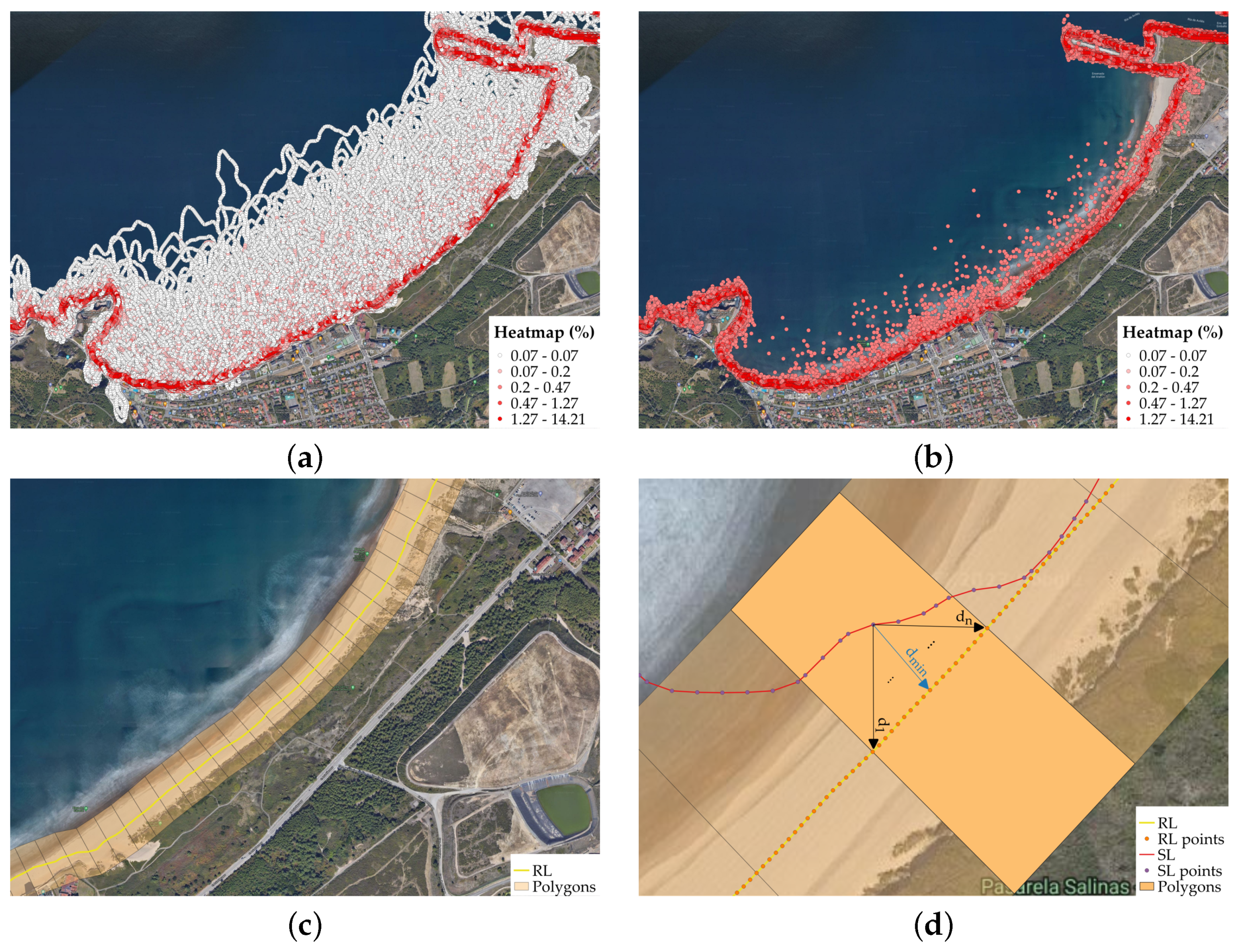
2.4.2. Shoreline Filtering Based on Distance from the Reference Line
2.5. Validation and Interpretation of SAR Shorelines and Change Rates
2.5.1. Bull Island
- 1.
- VL digitizing for each available image.
- 2.
- Position and measurement uncertainty calculation.
- 3.
- Quantifying SL change employing a dedicated software tool.
2.5.2. Salinas Beach
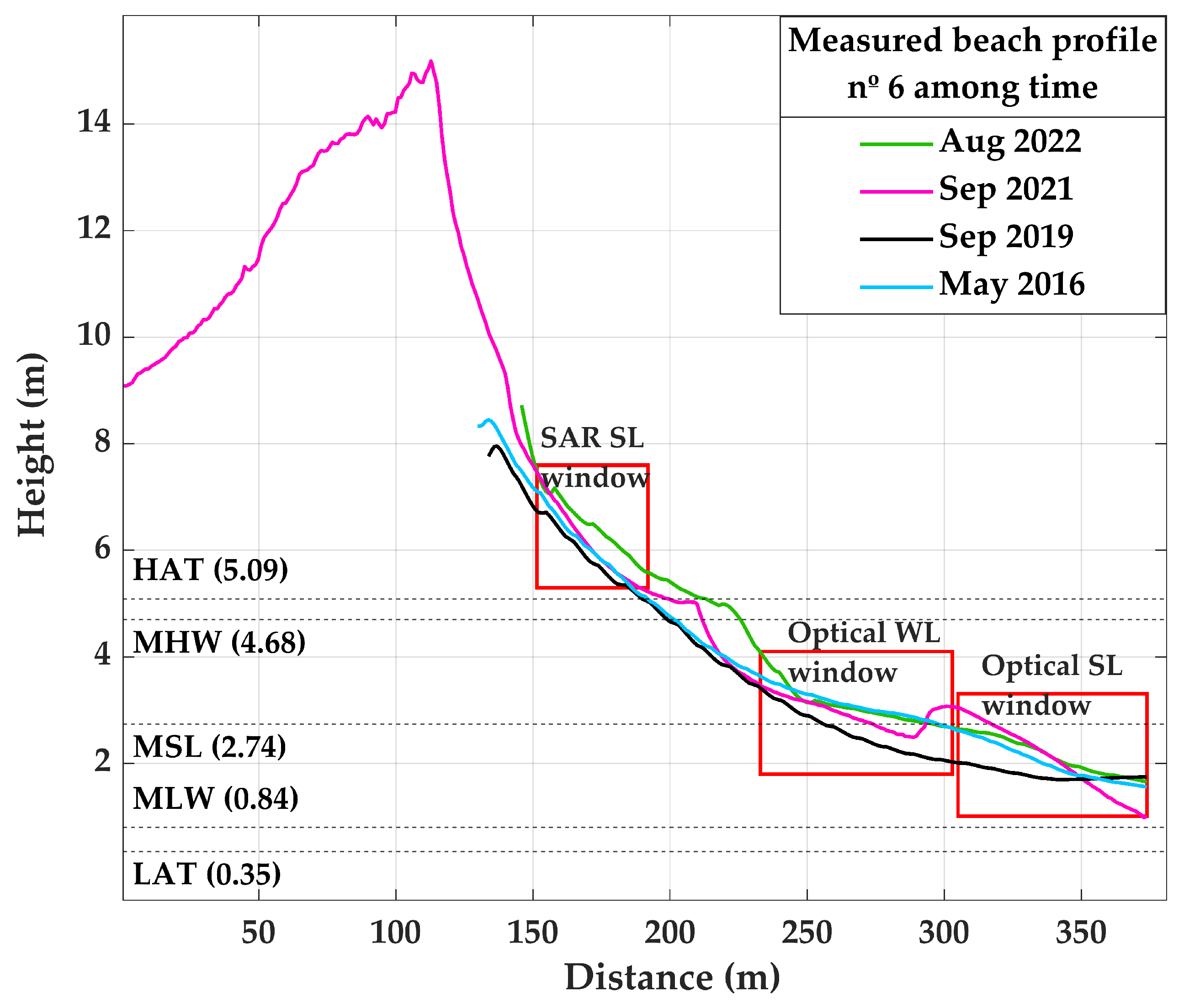
- Inter-annual changes based on a qualitative assessment of the erosional/accretional processes observed according to the SAR-SL distance from the baseline in comparison to those observed in topographic field surveys. The beach subaerial topography is monitored on a regular basis by means of in situ surveys provided by the Ministry of the Ecological Transition and the Demographic Challenge of the Government of Spain with a variable precision ranging from 10 to 0.1 m. Four surveys are available since 2015: May 2016, September 2019, September 2021, and August 2022. The topographic surveys cover the beach foreshore and backshore, including the inter-tidal area, berm, and dry beach, up to the toe of the dune or seawall. The survey dated September 2021 also covers the dune seaward slope and crest. From these topographic surveys, the shape of the beach profile is extracted along transects placed in the center of polygons (Figure 7). The vertical reference level for these topographic surveys (chart datum of Avilés Port) is located 274 cm below the local mean sea level. Other vertical references, such as the highest astronomical tide, mean high water, mean low water, and the lowest astronomical tide, are shown in Figure 8 with results of the topographic surveys for beach profile No. 6 as an example, along with the window that indicates where SAR-SLs are identified.
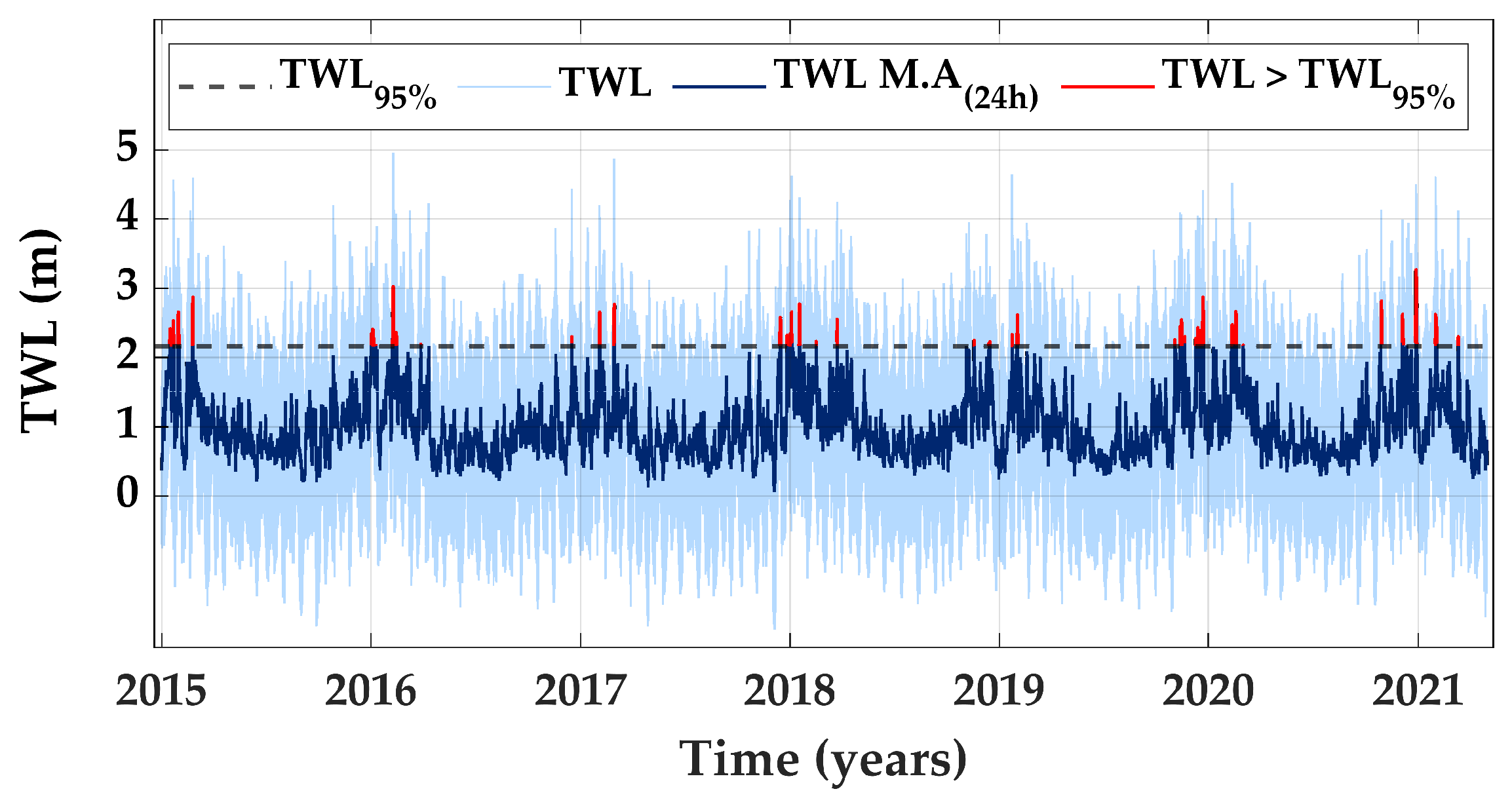
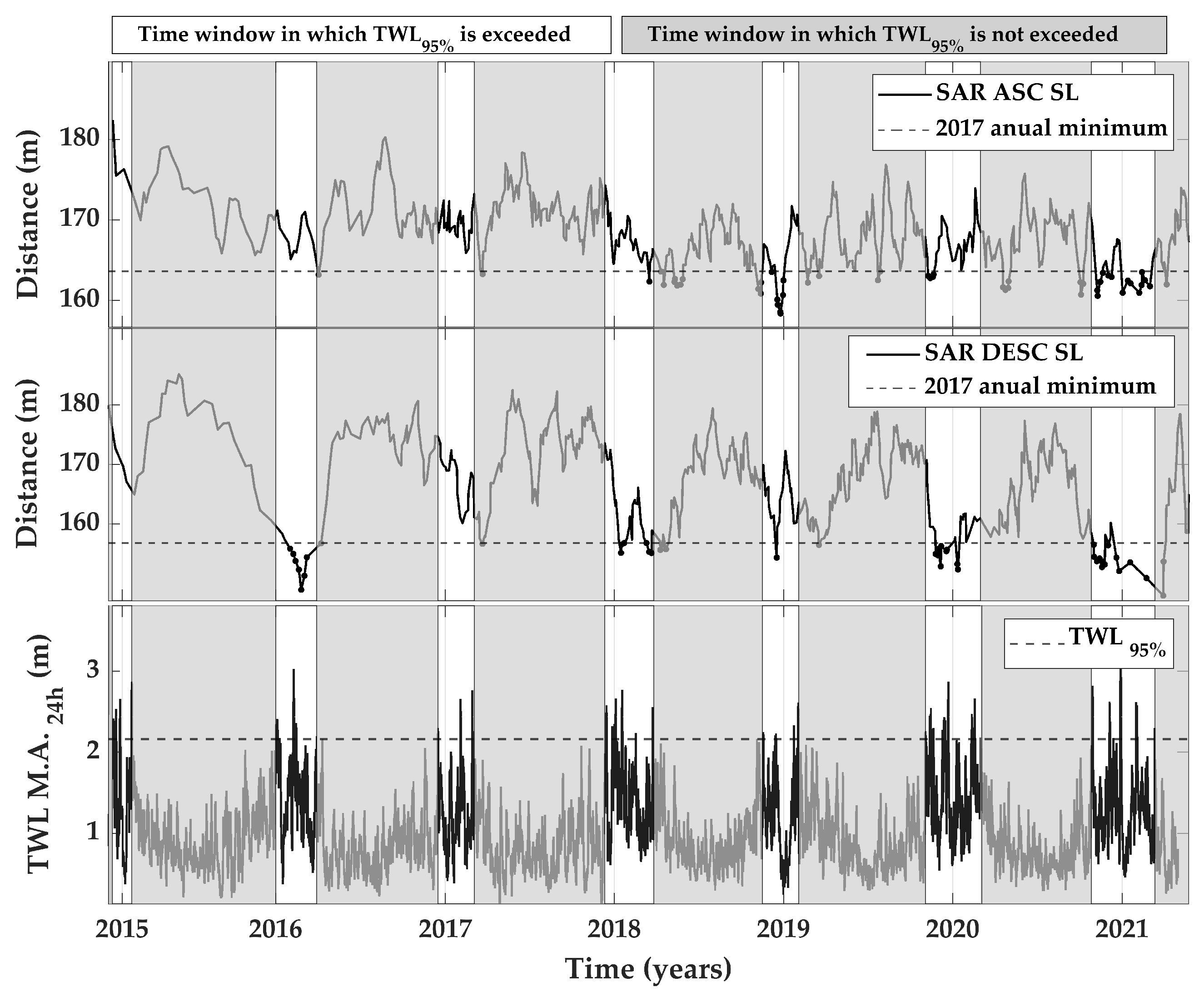
- Seasonal changes, based on the correlation between the time series of SAR-SL position (distance from the baseline) and local hydrodynamics. Time series of wave parameters, tides, and surge levels are obtained from the databases Global Ocean Waves [39], Global Ocean Tides [40], and Global Ocean Surges [41], respectively (see time series in Figure A1). Regarding waves, the Global Ocean Waves dataset consists of hindcast data generated with the WaveWatch III numerical model. In the study area, the dataset spans from 1979 to 2021 with a temporal resolution of one hour and a spatial resolution of 0.25 degrees. Regarding the astronomical tide, the Global Ocean Tides provides hourly time series of astronomical tides with global coverage and a spatial resolution of 0.25 degrees. Astronomical tides are generated from the harmonic constants derived from the TPXO global tide model in its different versions developed by Oregon State University. As for the storm surge, the Global Ocean Surges dataset is a hindcast storm surge dataset generated with the Regional Ocean Model System, which is a three-dimensional oceanic model that solves the Reynolds-averaged Navier–Stokes equations using the Boussinesq approximation. In the study area, the dataset spans from 1985 to 2020 with a temporal resolution of one hour and a spatial resolution of 0.08 degrees.
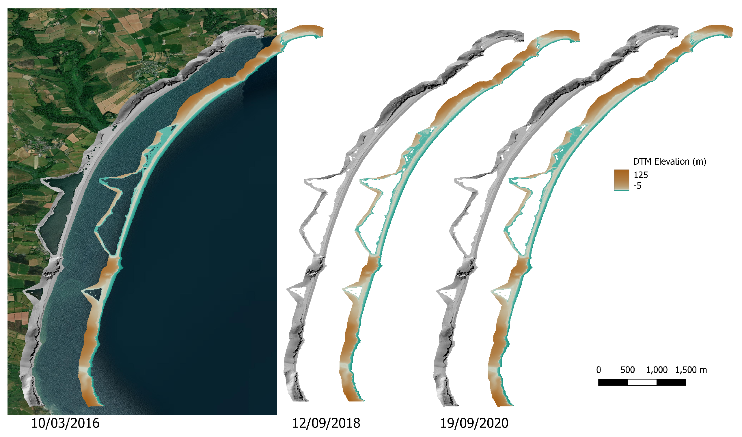
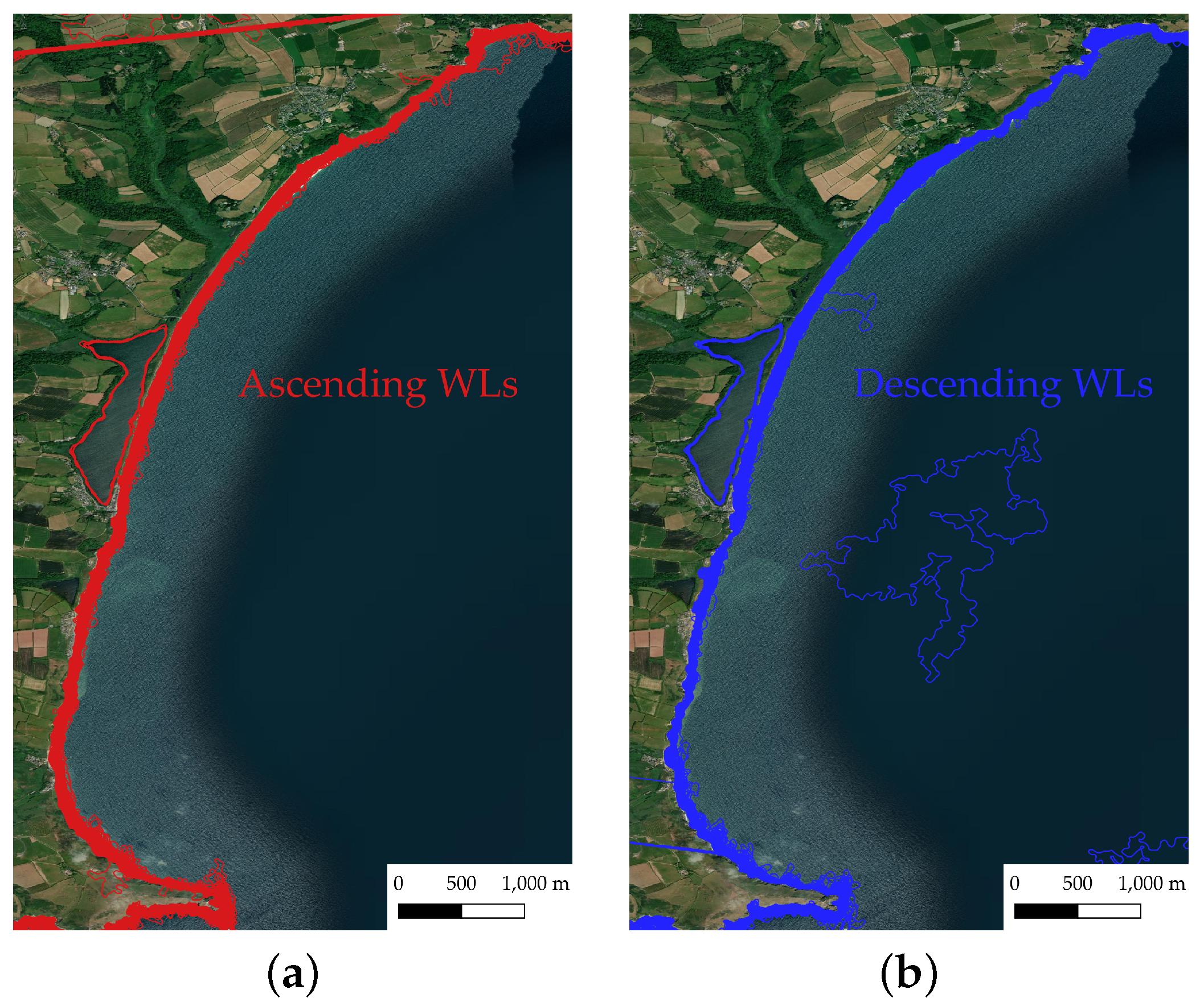
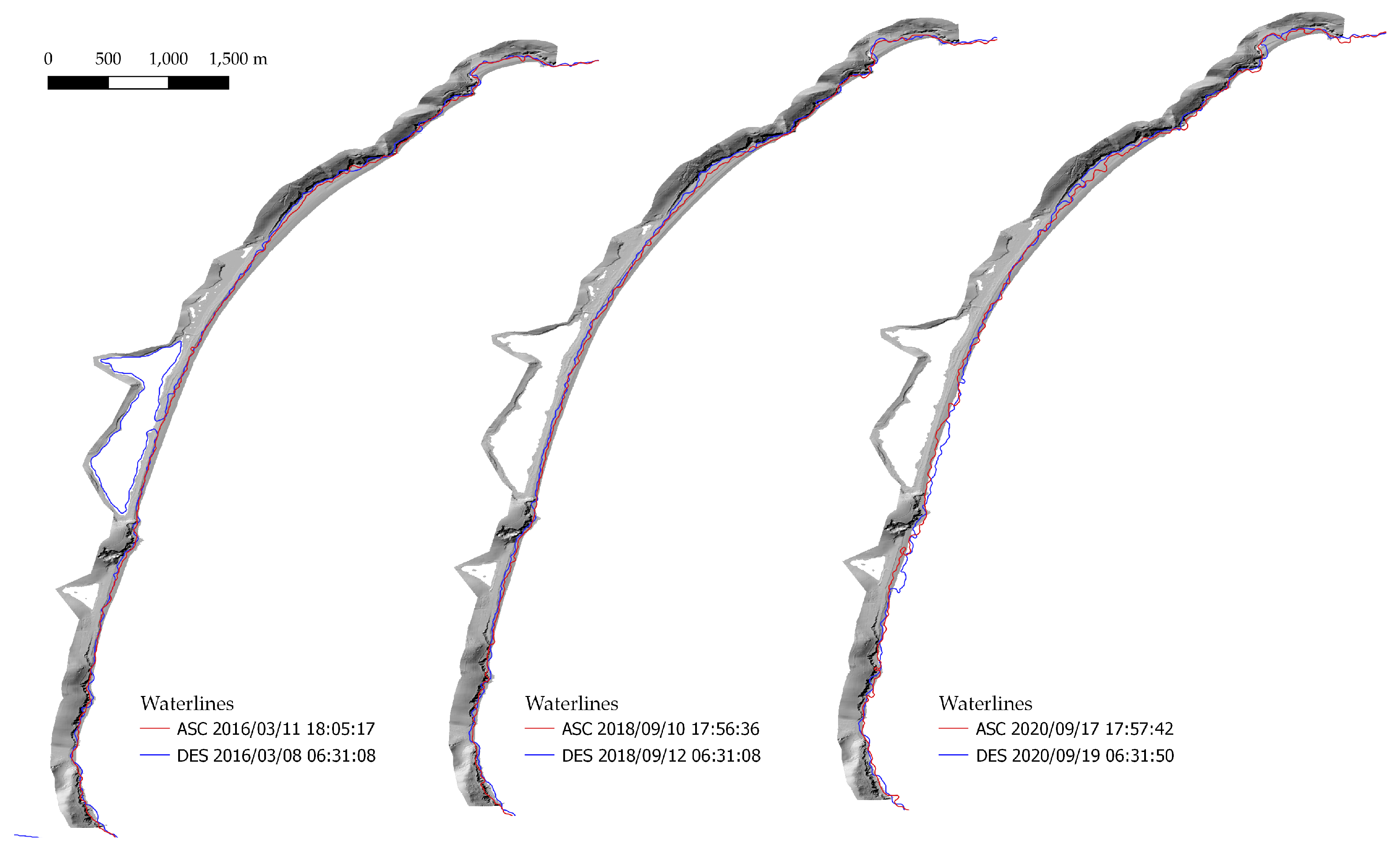
2.5.3. Start Bay
3. Results
3.1. Bull Island
3.2. Salinas Beach
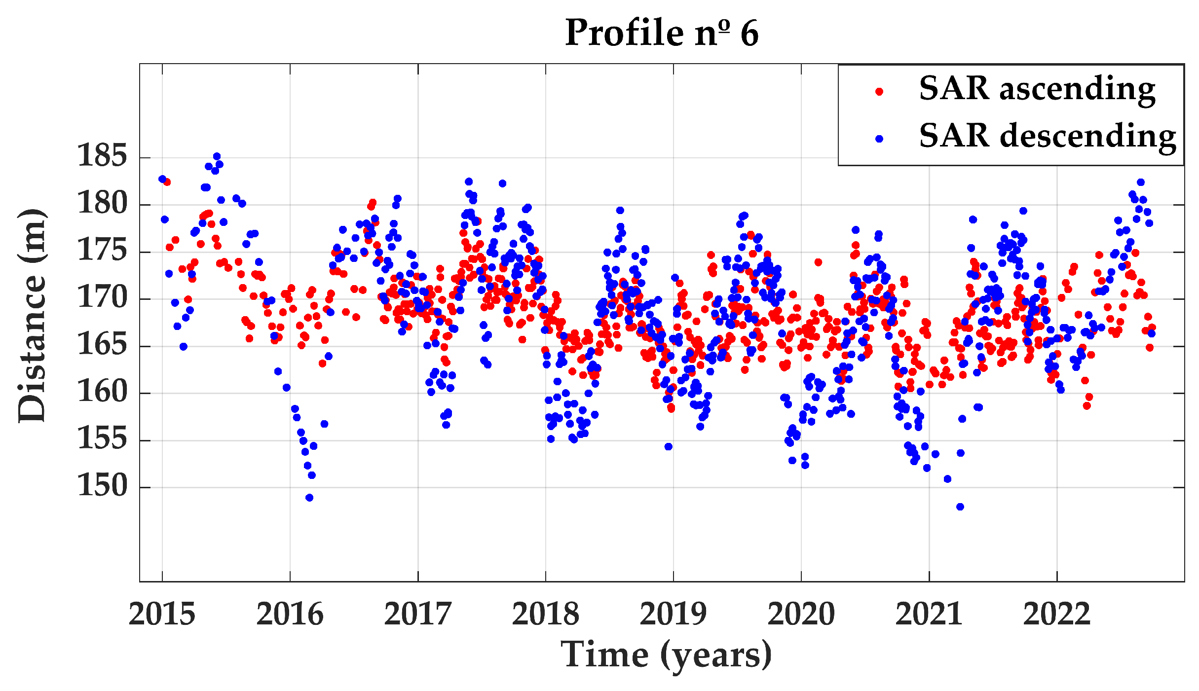
3.2.1. Seasonality in Salinas SAR-SL
3.2.2. Inter-Annual Changes in Salinas SAR-SL
- In May 2016, the beach profile was in an intermediate position.
- In September 2019, the beach profile migrated inland, showing maximum beach erosion.
- In September 2021, the beach profile came back to an intermediate position, like in May 2016.
- In August 2022, the beach profile migrated seaward, showing maximum beach accretion.
3.2.3. Change Detection from Optical WLs in Salinas
- In May 2016, the beach profile was in the most advanced position, showing maximum beach accretion.
- In September 2019, the beach profile migrated inland, showing maximum beach erosion.
- In September 2021, the beach profile migrated seaward to an intermediate position.
- In August 2022, the beach profile migrated further seaward, showing maximum beach accretion, like in May 2016.
3.3. Start Bay
4. Discussion
4.1. The Influence of Met-Ocean Conditions
4.2. The Influence of Soil Moisture
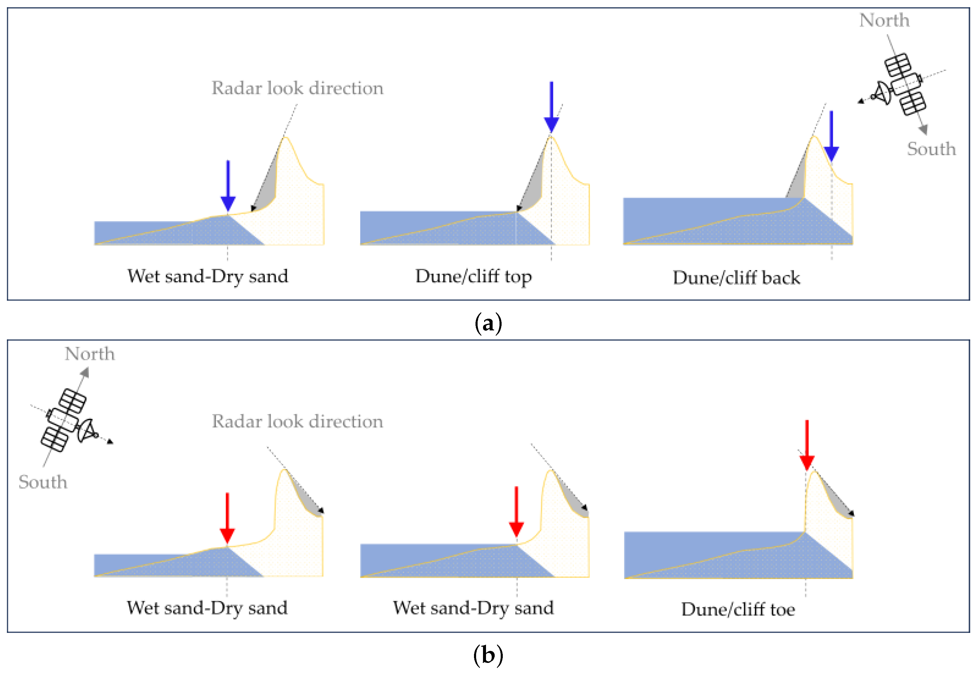
4.3. The Influence of Scene Geometry
4.4. Interpretation of SAR-SLs
4.5. Limitations of This Study
5. Conclusions
Author Contributions
Funding
Data Availability Statement
Acknowledgments
Conflicts of Interest
Abbreviations
| ASC | Ascending |
| CR | Change rate |
| DESC | Descending |
| DoD | Digital elevation model of difference |
| DSAS | Digital Shoreline Analysis System |
| DTM | Digital terrain model |
| SAR | Synthetic aperture radar |
| ESA | European Space Agency |
| GMD | Gaussian mixture distribution |
| GRD | Ground Range Detected |
| RL | Reference line |
| SL | Shoreline |
| S1 | Sentinel-1 |
| S2 | Sentinel-2 |
| TWL | Total water level |
| VL | Vegetation line |
Appendix A


References
- Mingle, J. The Ocean and Cryosphere in a Changing Climate: Special Report of the Intergovernmental Panel on Climate Change (IPCC); Cambridge University Press: Cambridge, UK, 2022. [Google Scholar] [CrossRef]
- Anfuso, G.; Bowman, D.; Danese, C.; Pranzini, E. Transect based analysis versus area based analysis to quantify shoreline displacement: Spatial resolution issues. Environ. Monit. Assess. 2016, 188, 568. [Google Scholar] [CrossRef] [PubMed]
- Boak, E.H.; Turner, I.L. Shoreline Definition and Detection: A Review. J. Coast. Res. 2005, 2005, 688–703. [Google Scholar] [CrossRef]
- Toure, S.; Diop, O.; Kpalma, K.; Maiga, A.S. Shoreline Detection using Optical Remote Sensing: A Review. ISPRS Int. J.-Geo-Inf. 2019, 8, 12876. [Google Scholar] [CrossRef]
- Luijendijk, A.; Hagenaars, G.; Ranasinghe, R.; Baart, F.; Donchyts, G.; Aarninkhof, S. The state of the world’s beaches. Sci. Rep. 2018, 8, 6641. [Google Scholar] [CrossRef] [PubMed]
- Mentaschi, L.; Vousdoukas, M.I.; Pekel, J.F.; Voukouvalas, E.; Feyen, L. Global long-term observations of coastal erosion and accretion. Sci. Rep. 2018, 8, 12876. [Google Scholar] [CrossRef] [PubMed]
- Muttitanon, W.; Tripathi, N.K. Land use/land cover changes in the coastal zone of Ban Don Bay, Thailand using Landsat 5 TM data. Int. J. Remote Sens. 2005, 26, 2311–2323. [Google Scholar] [CrossRef]
- Hagenaars, G.; Luijendijk, A.; de Vries, S.; de Boer, W. Long term coastline monitoring derived from satellite imagery. In Proceedings of the 8th International Conference on Coastal Dynamics, Helsingør, Denmark, 12–16 June 2017; pp. 1551–1562. [Google Scholar]
- Maglione, P.; Parente, C.; Vallario, A. Coastline extraction using high resolution WorldView-2 satellite imagery. Eur. J. Remote Sens. 2014, 47, 685–699. [Google Scholar] [CrossRef]
- Ghosh, M.K.; Kumar, L.; Roy, C. Monitoring the coastline change of Hatiya Island in Bangladesh using remote sensing techniques. ISPRS J. Photogramm. Remote Sens. 2015, 101, 137–144. [Google Scholar] [CrossRef]
- Curlander, J.C.; McDonough, R.N. Synthetic Aperture Radar; Wiley: New York, NY, USA, 1991; Volume 11. [Google Scholar]
- Moreira, A.; Prats-Iraola, P.; Younis, M.; Krieger, G.; Hajnsek, I.; Papathanassiou, K.P. A tutorial on synthetic aperture radar. IEEE Geosci. Remote Sens. Mag. 2013, 1, 6–43. [Google Scholar] [CrossRef]
- Ulaby, F.T.; Long, D.G.; Blackwell, W.J.; Elachi, C.; Fung, A.K.; Ruf, C.; Sarabandi, K.; Zebker, H.A.; Van Zyl, J. Microwave Radar and Radiometric Remote Sensing; University of Michigan Press: Ann Arbor, MI, USA, 2014; Volume 4. [Google Scholar]
- Vos, K.; Harley, M.D.; Splinter, K.D.; Simmons, J.A.; Turner, I.L. Sub-annual to multi-decadal shoreline variability from publicly available satellite imagery. Coast. Eng. 2019, 150, 160–174. [Google Scholar] [CrossRef]
- Paz-Delgado, M.V.; Payo, A.; Gómez-Pazo, A.; Beck, A.L.; Savastano, S. Shoreline Change from Optical and Sar Satellite Imagery at Macro-Tidal Estuarine, Cliffed Open-Coast and Gravel Pocket-Beach Environments. J. Mar. Sci. Eng. 2022, 10, 561. [Google Scholar] [CrossRef]
- Dike, E.C.; Oyetunji, A.K.; Amaechi, C.V. Shoreline Delineation from Synthetic Aperture Radar (SAR) Imagery for High and Low Tidal States in Data-Deficient Niger Delta Region. J. Mar. Sci. Eng. 2023, 11, 1528. [Google Scholar] [CrossRef]
- Gallagher, S.; Tiron, R.; Dias, F. A long-term nearshore wave hindcast for Ireland: Atlantic and Irish Sea coasts (1979–2012) Present wave climate and energy resource assessment. Ocean. Dyn. 2014, 64, 1163–1180. [Google Scholar] [CrossRef]
- Wright, L.; Short, A. Morphodynamic variability of surf zones and beaches: A synthesis. Mar. Geol. 1984, 56, 93–118. [Google Scholar] [CrossRef]
- Wiggins, M.; Scott, T.; Masselink, G.; Russell, P.; McCarroll, R.J. Coastal embayment rotation: Response to extreme events and climate control, using full embayment surveys. Geomorphology 2019, 327, 385–403. [Google Scholar] [CrossRef]
- McCarroll, R.; Valiente, N.; Wiggins, M.; Scott, T.; Masselink, G. Coastal survey data for Perranporth Beach and Start Bay in southwest England (2006–2021). Sci. Data 2023, 10, 258. [Google Scholar] [CrossRef]
- Chadwick, A.J.; Karunarathna, H.; Gehrels, W.R.; Massey, A.C.; O’Brien, D.; Dales, D. A new analysis of the Slapton barrier beach system, UK. Marit. Eng. 2005, 158, 147–161. [Google Scholar] [CrossRef]
- Ruiz de Alegria-Arzaburu, A.; Masselink, G. Storm response and beach rotation on a gravel beach, Slapton Sands, U.K. Mar. Geol. 2010, 278, 77–99. [Google Scholar] [CrossRef]
- Aulard-Macler, M. Sentinel-1 Product Definition; Document Reference MPC-0240; MacDonald, Dettwiler and Associates: Westminster, CO, USA, 2011. [Google Scholar]
- Zollini, S.; Alicandro, M.; Cuevas-González, M.; Baiocchi, V.; Dominici, D.; Buscema, P.M. Shoreline Extraction Based on an Active Connection Matrix (ACM) Image Enhancement Strategy. J. Mar. Sci. Eng. 2020, 8, 9. [Google Scholar] [CrossRef]
- Veci, L.; Lu, J.; Foumelis, M.; Engdahl, M. ESA’s Multi-mission Sentinel-1 Toolbox. In Proceedings of the EGU General Assembly Conference Abstracts, Vienna, Austria, 23–28 April 2017; p. 19398. [Google Scholar]
- Lee, J.S.; Wen, J.H.; Ainsworth, T.; Chen, K.S.; Chen, A. Improved Sigma Filter for Speckle Filtering of SAR Imagery. IEEE Trans. Geosci. Remote Sens. 2009, 47, 202–213. [Google Scholar] [CrossRef]
- Marghany, M.; Sabu, Z.; Hashim, M. Mapping coastal geomorphology changes using synthetic aperture radar data. Int. J. Phys. Sci 2010, 5, 1890–1896. [Google Scholar]
- Pradhan, B.; Rizeei, H.M.; Abdulle, A. Quantitative Assessment for Detection and Monitoring of Coastline Dynamics with Temporal RADARSAT Images. Remote Sens. 2018, 10, 1705. [Google Scholar] [CrossRef]
- Achim, A.; Tsakalides, P.; Bezerianos, A. SAR image denoising via Bayesian wavelet shrinkage based on heavy-tailed modeling. IEEE Trans. Geosci. Remote Sens. 2003, 41, 1773–1784. [Google Scholar] [CrossRef]
- Yu, Y.; Acton, S. Speckle reducing anisotropic diffusion. IEEE Trans. Image Process. 2002, 11, 1260–1270. [Google Scholar] [CrossRef] [PubMed]
- Kittler, J.; Illingworth, J. Minimum error thresholding. Pattern Recognit. 1986, 19, 41–47. [Google Scholar] [CrossRef]
- Serra, J. Image Analysis and Mathematical Morphology. Cytometry 1983, 4, 184–185. [Google Scholar]
- Maple, C. Geometric design and space planning using the marching squares and marching cube algorithms. In Proceedings of the 2003 International Conference on Geometric Modeling and Graphics, London, UK, 16–18 July 2003; pp. 90–95. [Google Scholar] [CrossRef]
- Schwarz, G. Estimating the Dimension of a Model. Ann. Stat. 1978, 6, 461–464. [Google Scholar] [CrossRef]
- Leatherman, S.P. Shoreline Change Mapping and Management Along the U.S. East Coast. J. Coast. Res. 2003, 5–13. [Google Scholar]
- Himmelstoss, E.; Henderson, R.E.; Kratzmann, M.G.; Farris, A.S. Digital Shoreline Analysis System (DSAS), Version 5.1 User Guide; Technical Report; U.S. Geological Survey: Reston, VA, USA, 2021. [CrossRef]
- Genz, A.S.; Frazer, L.N.; Fletcher, C.H. Improving Statistical Validity in Calculating Erosion Hazards from Historical Shorelines. In Coastal Sediments’ 07; American Society of Civil Engineers: Reston, VA, USA, 2007; pp. 1799–1812. [Google Scholar] [CrossRef]
- Hapke, C.J.; Himmelstoss, E.A.; Kratzmann, M.G.; List, J.H.; Thieler, E.R. National Assessment of Shoreline Change; Historical Shoreline Change along the New England and Mid-Atlantic Coasts; U.S. Geological Survey: Reston, VA, USA, 2011.
- Perez, J.; Menendez, M.; Losada, I.J. GOW2: A global wave hindcast for coastal applications. Coast. Eng. 2017, 124, 1–11. [Google Scholar] [CrossRef]
- Egbert, G.D.; Erofeeva, S.Y. Efficient Inverse Modeling of Barotropic Ocean Tides. J. Atmos. Ocean. Technol. 2002, 19, 183–204. [Google Scholar] [CrossRef]
- Cid, A.; Castanedo, S.; Abascal, A.J.; Menéndez, M.; Medina, R. A high resolution hindcast of the meteorological sea level component for Southern Europe: The GOS dataset. Clim. Dyn. 2014, 43, 2167–2184. [Google Scholar] [CrossRef]
- Vos, K.; Splinter, K.D.; Harley, M.D.; Simmons, J.A.; Turner, I.L. CoastSat: A Google Earth Engine-enabled Python toolkit to extract shorelines from publicly available satellite imagery. Environ. Model. Softw. 2019, 122, 104528. [Google Scholar] [CrossRef]
- Bell, C. POLTIPS. 3. Applications Team at the National Oceanographic Centre; National Oceanography Centre: Liverpool, UK, 2016. [Google Scholar]
- Turner, J.F.; Iliffe, J.C.; Ziebart, M.K.; Wilson, C.; Horsburgh, K.J. Interpolation of Tidal Levels in the Coastal Zone for the Creation of a Hydrographic Datum. J. Atmos. Ocean. Technol. 2010, 27, 605–613. [Google Scholar] [CrossRef]
- García, P.; Martin-Puig, C.; Roca, M. SARin mode, and a window delay approach, for coastal altimetry. Adv. Space Res. 2018, 62, 1358–1370. [Google Scholar] [CrossRef]
- Stockdon, H.F.; Holman, R.A.; Howd, P.A.; Sallenger, A.H. Empirical parameterization of setup, swash, and runup. Coast. Eng. 2006, 53, 573–588. [Google Scholar] [CrossRef]
- Sun, W.; Chen, C.; Yang, W.L.G.; Meng, X.; Wang, L.; Ren, K. Coastline extraction using remote sensing: A review. Gisci. Remote Sens. 2023, 60, 2243671. [Google Scholar] [CrossRef]
- Vrijling, J.; Meijer, G. Probabilistic coastline position computations. Coast. Eng. 1992, 17, 1–23. [Google Scholar] [CrossRef]
- Sletten, M.A.; Hwang, P.A. The Effect of Wind-Wave Growth on SAR-Based Waterline Maps. IEEE Trans. Geosci. Remote Sens. 2011, 49, 5140–5149. [Google Scholar] [CrossRef]
- Tajima, Y.; Wu, L.; Fuse, T.; Shimozono, T.; Sato, S. Study on shoreline monitoring system based on satellite SAR imagery. Coast. Eng. J. 2019, 61, 401–421. [Google Scholar] [CrossRef]
- Wu, L.; Tajima, Y.; Yamanaka, Y.; Shimozono, T.; Sato, S. Study on characteristics of SAR imagery around the coast for shoreline detection. Coast. Eng. J. 2019, 61, 152–170. [Google Scholar] [CrossRef]
- Zollini, S.; Dominici, D.; Alicandro, M.; Cuevas-González, M.; Angelats, E.; Ribas, F.; Simarro, G. New Methodology for Shoreline Extraction Using Optical and Radar (SAR) Satellite Imagery. J. Mar. Sci. Eng. 2023, 11, 627. [Google Scholar] [CrossRef]


| Bull Island | Salinas Beach | Start Bay | |
|---|---|---|---|
| Optical (S2) | 76 | 125 | 53 |
| SAR (S1) | 1055 | 1411 | 1402 |
| HR (m × m) | MR (m × m) | |
|---|---|---|
| SM | ||
| IW | ||
| EW |
| Date Acquisition | Source | Provider | Resolution (m × m) |
|---|---|---|---|
| 2 June 2016 | Google Earth Pro | SPOT 6 | |
| 7 May 2017 | Google Earth Pro | SPOT 7 | |
| 24 June 2018 | Google Earth Pro | WV2 Maxar technologies | |
| 1 June 2020 | Google Earth Pro | WV2 Maxar technologies | |
| 26 April 2021 | Google Earth Pro | WV2 Maxar technologies | |
| 28 March 2022 | Google Earth Pro | WV2 Maxar technologies |
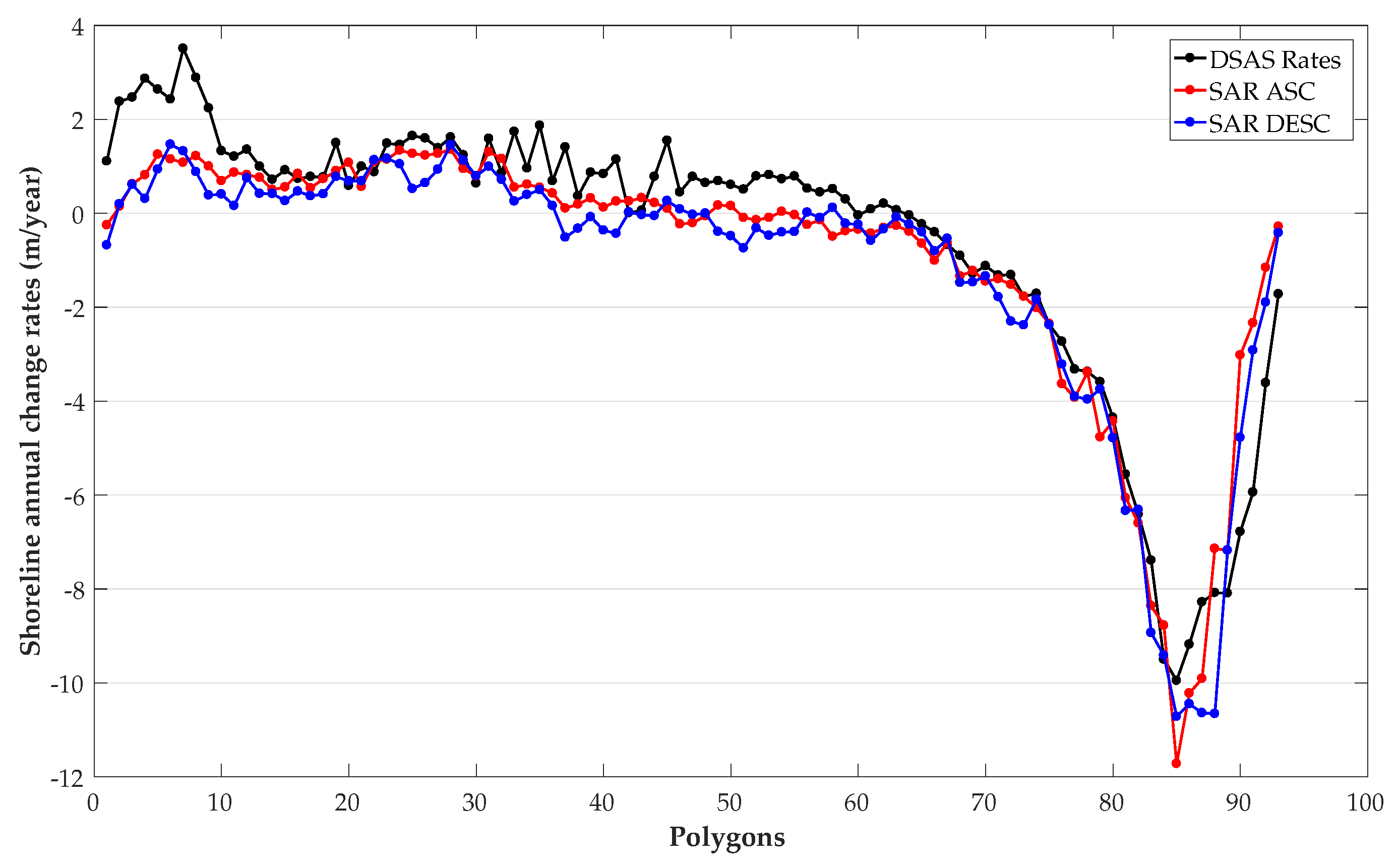
| SL Annual CRs | N | Mean | Max | Min | Advancing | Receding |
|---|---|---|---|---|---|---|
| SAR ASC | 93 | −0.95 | −11.72 | 1.36 | 47/93 | 46/93 |
| SAR DESC | 93 | −1.18 | −10.71 | 1.46 | 40/93 | 53/93 |
| VL DSAS | 93 | −0.54 | −9.95 | 3.51 | 62/93 | 31/93 |
| N | MAE | MAE (WLR < 0) | MAE (WLR > 0) | ||
|---|---|---|---|---|---|
| SAR ASC/ SAR DESC | 93 | 0.97 | 0.37 | - | - |
| VL DSAS/ SAR ASC | 93 | 0.90 | 0.75 | 0.83 | 0.70 |
| VL DSAS/ SAR DESC | 93 | 0.92 | 0.84 | 0.80 | 0.86 |
| Time Frame | SAR DESC SL | CoastSat WL |
|---|---|---|
| April–June 2016 | 9 | 7 |
| August–October 2019 | 31 | 8 |
| August–October 2021 | 29 | 3 |
| July–September 2022 | 14 | 10 |
| Total No. of records | 83 | 28 |
| SL Collection Date, Time, and Astronomical Tidal Level | ||
|---|---|---|
| DTM Collection Date | Ascending SLs | Descending SLs |
| 10 March 2016 | 11 March 2016 18:05:17 ↑ 1.1 m | 08 March 2016 06:31:08 ↓ 1.5 m |
| 12 September 2018 | 10 September 2018 17:56:36 ↑ 2.4 m | † 12 September 2018 06:31:08 ↑ 1.7 m |
| 19 September 2020 | 17 September 2020 17:57:42 2.7 m | † 19 September 2020 06:31:50 ↑ 2.2 m |
| SL Name | Count | Min (m) | Max (m) | Mean (m) | Std (m) | Median (m) |
|---|---|---|---|---|---|---|
| ASC 11 March 2016 ↑ | 10324 | −2.7 | 26.5 | 3.3 | 3.5 | 2.8 |
| ASC 10 September 2018 ↑ | 10311 | −2.1 | 50.0 | 4.2 | 6.3 | 3.1 |
| ASC 17 September 2020 | 8693 | −2.6 | 29.5 | 2.3 | 3.2 | 2.4 |
| DESC 08 March 2016 ↓ | 10826 | −2.5 | 44.0 | 4.6 | 6.5 | 3.2 |
| † DESC 12 September 2018 ↑ | 10147 | −2.2 | 40.6 | 4.6 | 5.5 | 3.8 |
| † DESC 19 September 2020 ↑ | 7791 | −2.7 | 36.8 | 3.5 | 5.3 | 2.8 |
Disclaimer/Publisher’s Note: The statements, opinions and data contained in all publications are solely those of the individual author(s) and contributor(s) and not of MDPI and/or the editor(s). MDPI and/or the editor(s) disclaim responsibility for any injury to people or property resulting from any ideas, methods, instructions or products referred to in the content. |
© 2024 by the authors. Licensee MDPI, Basel, Switzerland. This article is an open access article distributed under the terms and conditions of the Creative Commons Attribution (CC BY) license (https://creativecommons.org/licenses/by/4.0/).
Share and Cite
Savastano, S.; Gomes da Silva, P.; Sánchez, J.M.; Tort, A.G.; Payo, A.; Pattle, M.E.; Garcia-Mondéjar, A.; Castillo, Y.; Monteys, X. Assessment of Shoreline Change from SAR Satellite Imagery in Three Tidally Controlled Coastal Environments. J. Mar. Sci. Eng. 2024, 12, 163. https://doi.org/10.3390/jmse12010163
Savastano S, Gomes da Silva P, Sánchez JM, Tort AG, Payo A, Pattle ME, Garcia-Mondéjar A, Castillo Y, Monteys X. Assessment of Shoreline Change from SAR Satellite Imagery in Three Tidally Controlled Coastal Environments. Journal of Marine Science and Engineering. 2024; 12(1):163. https://doi.org/10.3390/jmse12010163
Chicago/Turabian StyleSavastano, Salvatore, Paula Gomes da Silva, Jara Martínez Sánchez, Arnau Garcia Tort, Andres Payo, Mark E. Pattle, Albert Garcia-Mondéjar, Yeray Castillo, and Xavier Monteys. 2024. "Assessment of Shoreline Change from SAR Satellite Imagery in Three Tidally Controlled Coastal Environments" Journal of Marine Science and Engineering 12, no. 1: 163. https://doi.org/10.3390/jmse12010163
APA StyleSavastano, S., Gomes da Silva, P., Sánchez, J. M., Tort, A. G., Payo, A., Pattle, M. E., Garcia-Mondéjar, A., Castillo, Y., & Monteys, X. (2024). Assessment of Shoreline Change from SAR Satellite Imagery in Three Tidally Controlled Coastal Environments. Journal of Marine Science and Engineering, 12(1), 163. https://doi.org/10.3390/jmse12010163