Article

Research on the Heterogeneous Autonomous Underwater Vehicle Cluster Scheduling Problem Based on Underwater Docking Chambers

1
School of Mechanical Engineering, Jiangsu University of Science and Technology, Zhenjiang 212003, China
2
Marine Equipment and Technology Institute, Jiangsu University of Science and Technology, Zhenjiang 212003, China
3
708th Research Institute of CSSC, Huangpu District, Shanghai 200011, China
4
Shanghai Marine Equipment Research Institute, Shanghai 200031, China
*
Author to whom correspondence should be addressed.
J. Mar. Sci. Eng. 2024, 12(1), 162; https://doi.org/10.3390/jmse12010162
Submission received: 18 December 2023 / Revised: 9 January 2024 / Accepted: 12 January 2024 / Published: 14 January 2024
(This article belongs to the Section Ocean Engineering)

Abstract

:
The onboard energy supply of Autonomous Underwater Vehicles (AUVs) is one of the main limiting factors for their development. The existing methods of deploying and retrieving AUVs from mother ships consume a significant amount of energy during submerging and surfacing, resulting in a small percentage of actual working time. Underwater docking chambers provide support to AUVs underwater, saving their precious energy and addressing this issue. When an AUV cluster is assigned multiple tasks, scheduling the cluster becomes essential, and task allocation and path planning are among the core problems in AUV cluster scheduling research. In this paper, based on the underwater docking chamber, an Improved Genetic Local Search Algorithm with Prior Knowledge (IGLSAPK) is proposed to simultaneously solve the task allocation and path planning problems. Under constraints such as onboard energy supply, AUV quantity, and AUV type, the algorithm groups AUVs, assigns tasks, and plans paths to accomplish tasks at different locations, aiming to achieve overall efficiency. The algorithm first generates an initial population using prior knowledge to improve its search efficiency. It then combines an improved local search algorithm to efficiently solve large-scale, complex, and highly coupled problems. The algorithm has been evaluated through simulation experiments and comparative experiments, and the results demonstrate that the proposed algorithm outperforms other algorithms in terms of speed and optimality. The algorithm presented in this paper addresses the grouping, task allocation, and path planning problems in heterogeneous AUV clusters. Its practical significance lies in its ability to handle tasks executed by a heterogeneous AUV group, making it more practical compared to previous algorithms.

1. Introduction

In recent years, the application of Autonomous Underwater Vehicles (AUVs) has become increasingly widespread, and the tasks they need to complete have become more complex. They are extensively utilized in marine surveys, mapping, environmental monitoring, search operations, oil and gas exploration, and for inspections of underwater pipelines and infrastructure. Due to limitations in space payloads, energy, and costs, a single AUV cannot complete complex underwater missions effectively. An AUV cluster is a system composed of multiple AUVs. AUV clusters can accomplish complex tasks more efficiently and robustly. However, the traditional method of deploying and recovering AUVs from a mother ship requires high sea conditions, which results in high costs and involves certain unknown risks. The development of AUV clusters has greatly increased the number of AUVs, posing significant challenges in deploying and recovering them. The emergence of underwater docks has eased this problem. By using an underwater dock, multiple AUVs can be deployed and recovered at once. Energy supply, data collection, maintenance and repair, and other operations can be performed on AUVs underwater. This approach provides a relatively stable underwater environment, greatly improving the reliability and safety of AUV deployment and recovery. Additionally, AUVs do not need to frequently surface or submerge, saving precious onboard energy. Based on underwater docks, the scientific scheduling of AUV clusters is required for multiple task demands.

1.1. AUV Cluster Scheduling

AUV cluster scheduling refers to the assignment of tasks, path planning, and coordinated control of a cluster composed of multiple AUVs. In order to improve the efficiency of the overall mission, the allocation of tasks for multiple AUVs is determined based on the cost and requirements of each task [1,2]. The problem studied in this paper consists of three parts: heterogeneous AUV cluster grouping, task allocation within AUV teams, and path planning. These three parts have been extensively researched, but their interdependence poses significant challenges in solving the problem. They cannot be addressed separately and require comprehensive consideration.
AUV cluster task allocation can be divided into two methods: centralized and distributed. The centralized task allocation method requires each AUV to send information about its environment and the cost function for task execution to a central control center. The control center then considers the AUVs and tasks to make reasonable assignments [3]. After obtaining the positions and statuses of all AUVs in the system, the control center allocates the tasks based on their requirements. The objective is to minimize overall consumption or travel distance. This means that AUVs only participate in the “execution” step and not the “decision-making” step. The main centralized allocation methods include model-based linear programming methods [4], objective clustering methods [5], genetic algorithms [6], ant colony algorithms [7], particle swarm optimization [8], firefly algorithm [9], etc. [10]. This method heavily relies on underwater communication and puts a heavy computational burden on the control center. Therefore, it is preferred in situations with good communication conditions and low computational complexity. The distributed allocation method, on the other hand, involves AUVs communicating and “negotiating” with each other to formulate allocation plans and then execute them. It can also be referred to as decentralized allocation. The advantage of the distributed allocation method is that it ensures maximum efficiency for individual AUVs and fully utilizes the intelligent elements of AUVs. This algorithm is widely used in the field of robotics, including applications in biological immune mechanisms [11], contract network algorithms [12], market auction algorithms [13], as well as algorithms suitable for multi-agent information communication, such as self-organizing maps (SOM) [14].
AUV clusters are divided into homogenous and heterogeneous types, and a complex task requires collaboration among AUVs with different payloads. In underwater environments, due to cost constraints, a single AUV cannot integrate all functions, and thus, multiple types of heterogeneous AUVs are needed to collaborate on tasks. Therefore, heterogeneous multi-AUV systems are receiving increasing attention. Reasonable AUV task allocation can improve the efficiency of multi-AUV collaborative work and reduce the cost of collaboration.
AUV clusters can be organized into master–slave and parallel configurations. In a master–slave AUV system, one or a few vehicles serve as the master AUV with high-precision equipment, while the remaining vehicles are configured as slave AUVs with lower-precision equipment. During collaborative navigation, the master AUV transmits its own position information to the slave AUVs. The slave AUVs utilize relevant acoustic devices to obtain distance information between themselves and the master AUV. They then combine this information to collaboratively correct their own error information, thereby improving the overall navigation accuracy. Master–slave AUV systems can balance navigation accuracy and equipment cost, making them widely applicable in practical scenarios.
For AUV path planning, there are currently many commonly used methods, such as the A* algorithm [15], genetic algorithms [6,16,17,18], Ant Colony Optimization [7,19,20,21,22], particle swarm optimization [19,23,24], and Differential Evolution [25,26,27]. With the increase in environmental complexity and uncertainty, the requirements for AUV path planning are becoming increasingly high [28,29]. In recent years, with the development of deep neural networks, some self-learning methods, such as ones involving neural networks [30,31] and reinforcement learning [32,33,34], have been introduced into AUV local path planning. Deep reinforcement learning [35,36] combines deep neural networks and reinforcement learning techniques and has also been proposed and applied to AUV local path planning [37].

1.2. Challenges and Innovations

The following issues need to be resolved:
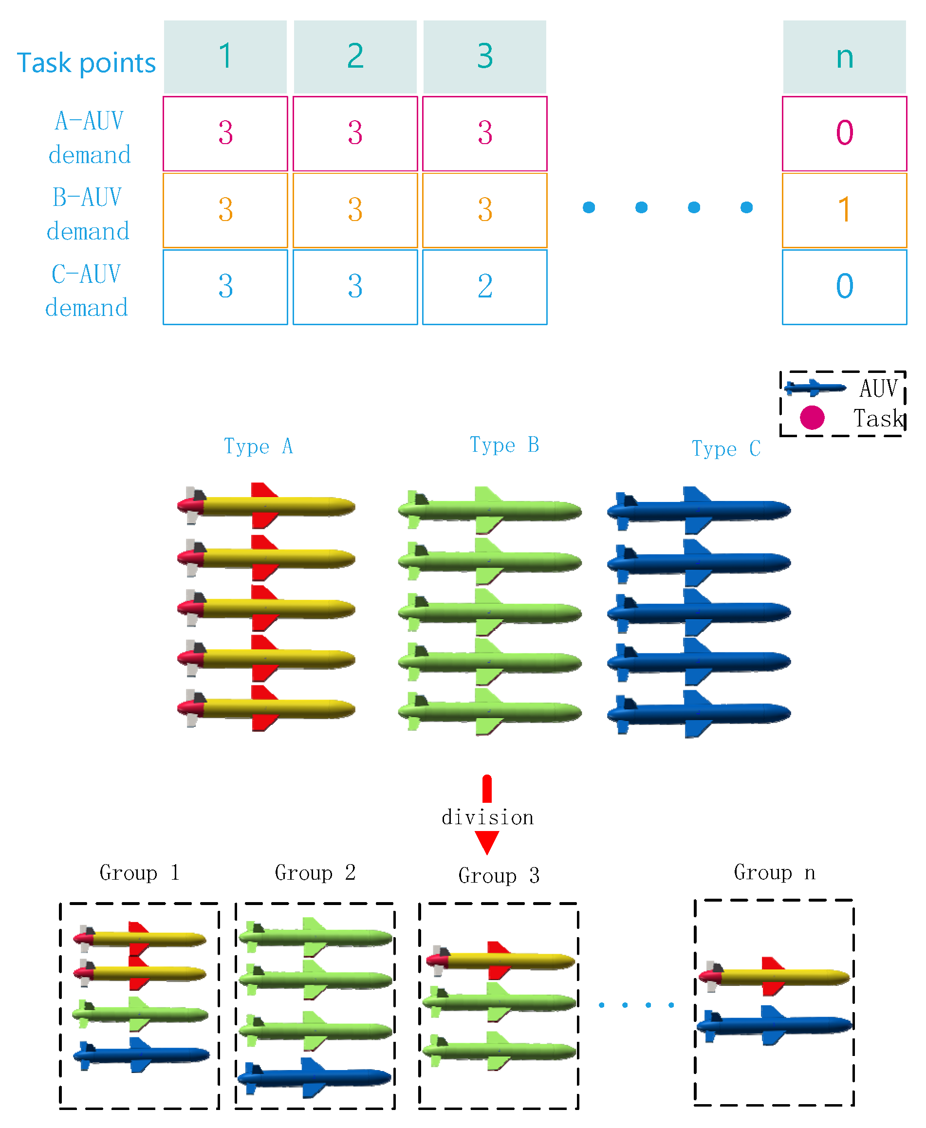
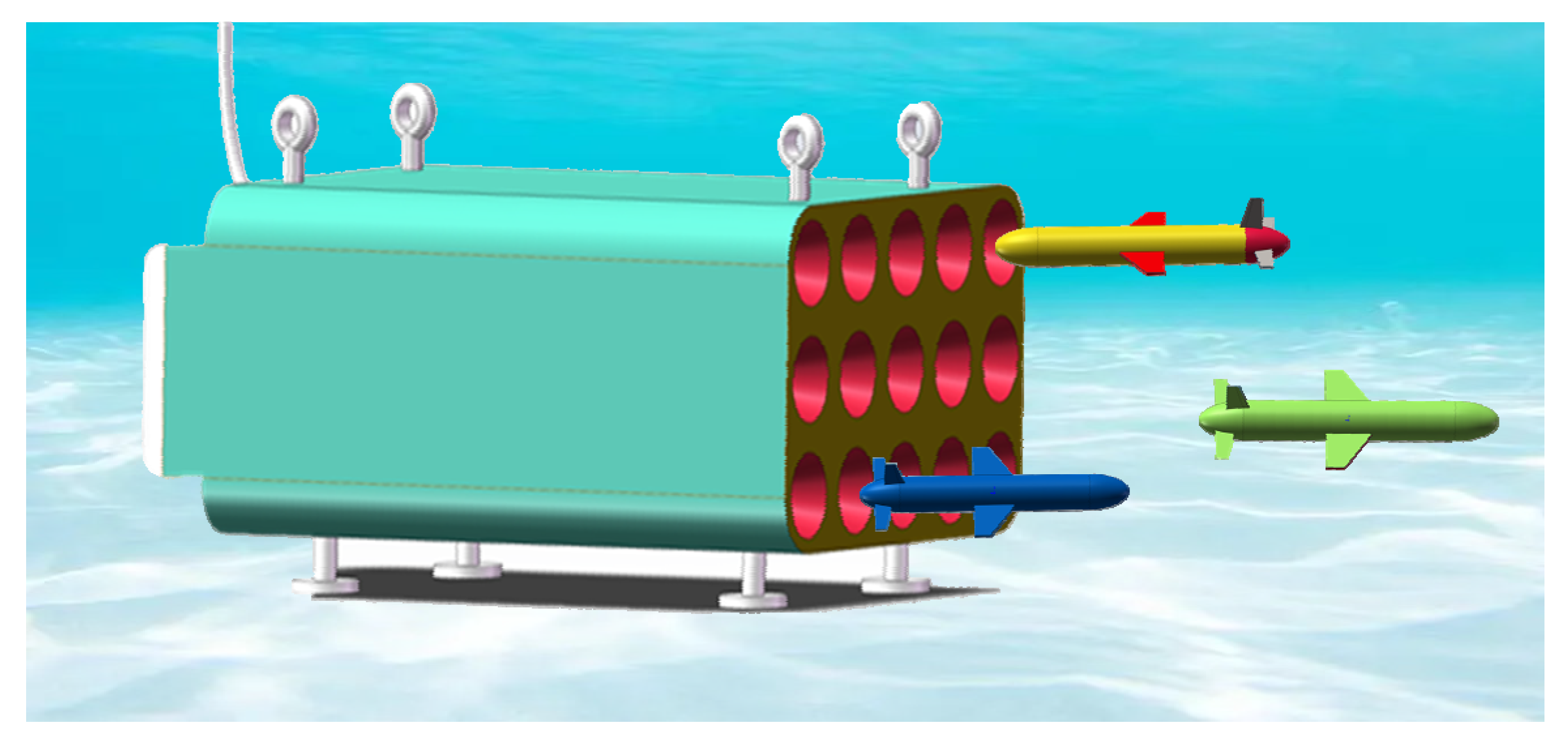
  • How to group limited AUVs to complete all tasks with different requirements at each task point while minimizing the overall cost? See Figure 1.
2.
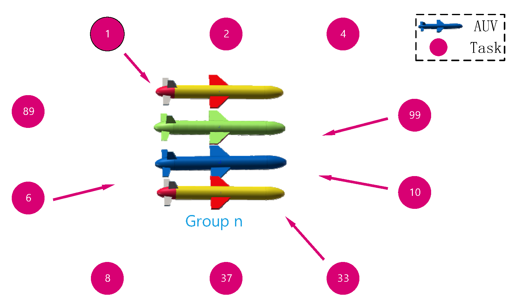
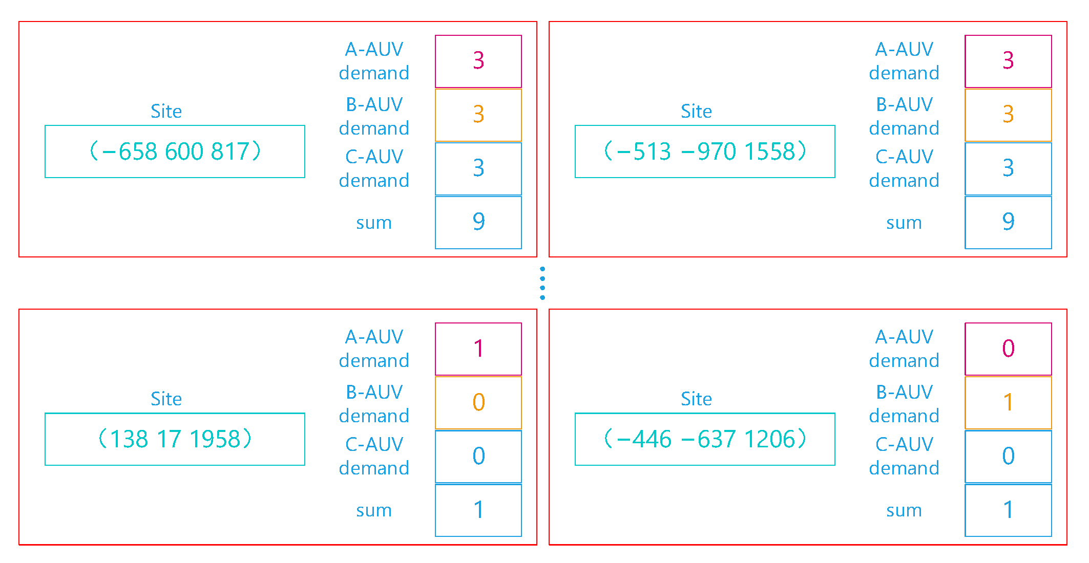
In cases with different requirements at each task point and with limitations on the energy carried by the vessel, there is an issue with respect to how different task points should be allocated to multiple AUV teams to ensure that overall consumption is minimized. See Figure 2.
3.
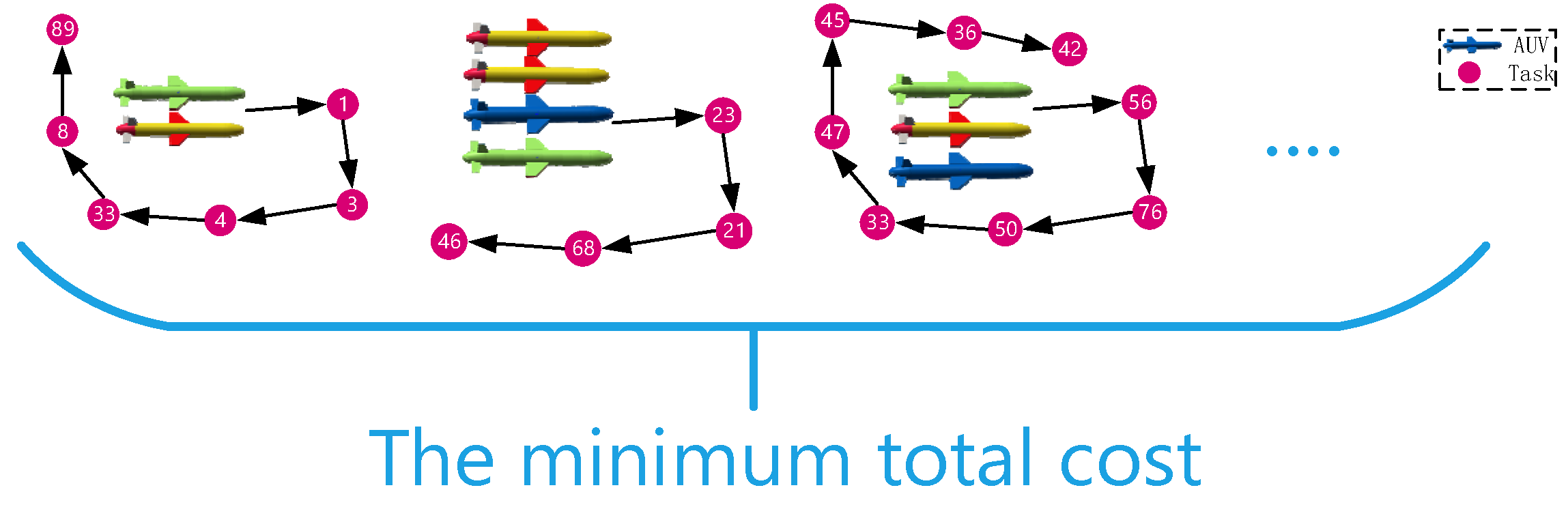
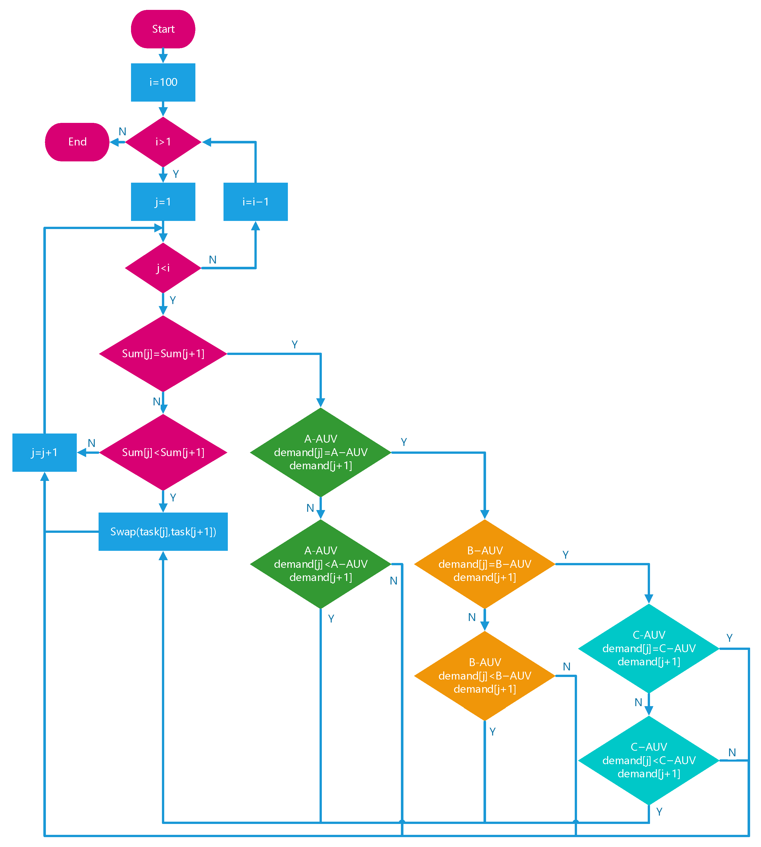
There is also an issue regarding the sorting of tasks while ensuring that the relevant requirements are met to find the optimal solution, as shown in Figure 3.
4.
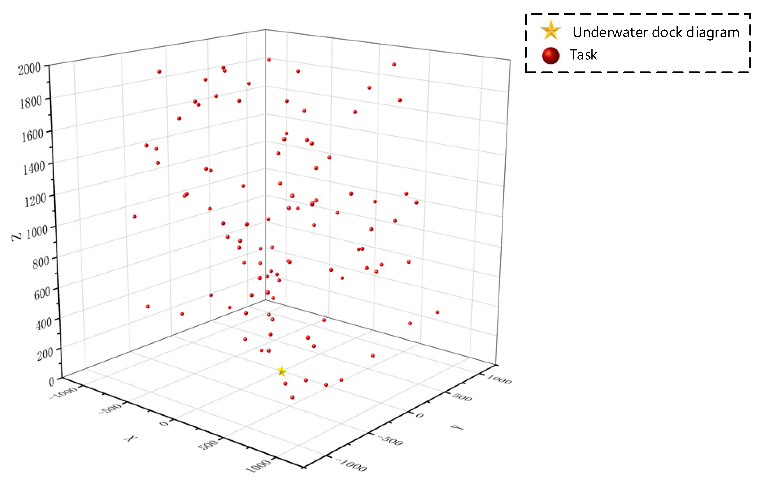
In a scenario where all tasks need to be completed, the objective is to minimize overall consumption, as shown in Figure 4.
The proposed algorithm has the following characteristics.
  • The proposed algorithm simultaneously addresses the issues of AUV grouping, task allocation, and path planning.
  • By using prior experience to generate an initial population and incorporating local search algorithms, the efficiency of the algorithm is significantly improved.
  • The algorithm is based on underwater docks, which is in line with the current trend of AUV deployment and retrieval, making it more practical.

2. The Optimization Model and Its Constraints

2.1. Problem Description

There are multiple tasks distributed across different locations within a certain area, as shown in Figure 5. Each task has specific requirements in terms of AUV models and quantities. The underwater dock houses several AUVs of different models, and the tasks require different quantities and types of AUVs to work together in teams. Therefore, it is necessary to group the AUVs, as shown in Figure 6. The onboard energy of the AUVs is limited, and if the energy is not sufficient for covering the energy consumption for traveling to the next location and returning, the AUVs will need to return to the dock for energy replenishment. The objective is to complete all tasks while minimizing overall cost.
The completion of tasks can be divided into three parts: AUV grouping, task allocation, and path planning. AUV grouping involves grouping AUVs of different quantities and types. Task allocation involves assigning different tasks to AUV teams. Path planning involves determining the order in which tasks are completed. Each part is strongly coupled and has a significant impact on the others. The grouping and task allocation are constrained by the availability of AUV quantities and types at each task point, while the path planning is constrained by energy availability. Each part influences the others greatly, and the previous task allocation and path planning decisions have a significant impact on subsequent tasks. To achieve minimal overall consumption, both task allocation and path planning need to be reasonable and coordinated with each other.

2.2. Modeling

Assumption: There are three types of AUVs, namely A, B, and C, in the underwater dock. Each type of AUV has a different payload capacity and is used to fulfill various task requirements. Specifically,
AUV = { AUV 1 ,   AUV 2 ,   AUV 3 ,   , AUV i }
In this formula, “i” represents the index of the AUV. The AUVs are typically sorted in the order of A, B, and C models.
According to the actual requirements, tasks are decomposed into different types of task sets:
mission = { mission 1 ,   mission 2 ,   mission j }
where j represents the index of the task.
Different types of tasks also require different types and quantities of AUVs. Often, a single task requires the collaboration of multiple AUV models.
mission j = { AUV j n 1 A , AUV j n 2 B , AUV j n 3 C , Mission _ Energy j , site ( x , y , z ) j }
In the above expression, “j” denotes the task number, “n” represents the required quantity, M i s s i o n _ E n e r g y j indicates the energy consumed for the completion of this task by an AUV. It is assumed that each AUV model consumes the same amount of energy for the same task. site ( x , y , z ) j represents the location of the task, with the underwater dock being set as the origin, denoted as site ( 0 , 0 , 0 ) O .
To determine a set of AUV deployments based on the requirements of task mission j .
A U V _ s w a r m j = { A U V i 1 , A U V i 2 , A U V i 3 , ...... }
A U V _ s w a r m j denotes the configuration of the AUV for the j-th mission, while A U V i with i indicates the i-th AUV.
Define the decision variable h j , which represents whether mission j is completed. A value of 1 indicates that mission j has been completed; otherwise, it indicates that it has not been completed.
h j = { 1 , C o m p l e t e   t h e   m i s s i o n ; 0 , F a i l   t o   c o m p l e t e   t h e   m i s s i o n .
Each goal includes tasks that must be executed, totaling M tasks; that is,
j = 1 M h j = M
With the prerequisite of completing all tasks, the objective is to minimize costs, primarily focusing on time to achieve the shortest overall duration.
Cost = min j = 1 M h _ cos t j
where Cos t represents the overall time cost, and h _ cos t j denotes the time spent from site ( x , y , z ) j 1 to site ( x , y , z ) j to reach and complete the task.
Define the decision variable x ( i , j ) to represent whether m i s s i o n j is executed. A value of 1 indicates that m i s s i o n j is executed for A U V i ; otherwise, it indicates that it is not executed.
x ( i , j ) = { 1 , A U V i m i s s i o n j ; 0 , o t h e r .
At the same moment, a task can be executed by multiple AUVs; that is,
i = 1 n x ( i , j ) 1 , j = 1 , 2 , , M .
At the same moment, any given AUV can only execute one task; that is,
j = 1 n x ( i , j ) 1 , i = 1 , 2 , , N .
The same AUV can execute a specific task only once; that is,
c = 1 C x ( i , j ) 1 .
where c represents the number of times an AUV performs the same task.
When a group of AUVs is assigned a set of tasks, each AUV needs to assess its energy status before undertaking the next task. The energy level after completing the subsequent task should be sufficient for supporting its return. It is required that each AUV in the group satisfies this constraint. If any AUV fails to meet this requirement, the entire group must return.
E _ r e m a i n j i E _ path j j + 1 i + E _ m i s s i o n j + 1 i + E _ b a c k j + 1 i ,   i = 1 , 2 , N ; j = 1 , 2 , M .
where E _ r e m a i n j i represents the remaining energy of AUV i after completing task j, E _ path j j + 1 i denotes the energy consumed in reaching the next task point, E _ m i s s i o n j + 1 i represents the energy consumed by AUV i in executing task j, and E _ b a c k j + 1 i stands for the energy consumed by AUV i in returning to the underwater dock at task point j + 1.
After completing a task and returning to the underwater dock, the AUV will undergo energy replenishment, data exchange, and maintenance. Assuming different AUV models consume the same amount of time and the duration is fixed, upon completing charging and maintenance, the AUVs will be reorganized based on the task requirements to continue task execution. Min T = 120   min .The time required for this process is at least 120 min, with no specified maximum duration.
t j + 1 D t j A 120
where the unit is in minutes, t j + 1 D represents the moment of leaving the dock and commencing the j + 1 task, and t j A represents the moment of completing the j task and arriving at the dock. The time spent by the AUV entering and leaving the dock is entirely encompassed within M i n T .
The successful completion of the task relies on three underlying assumptions. These are as follows:
Assumption 1.
The marine environment is stable, and there is no interference from ocean currents.
Assumption 2.
All target points are reachable, and there are no obstacles blocking the path.
Assumption 3.
AUVs of different models consume the same amount of energy under the same range of navigation.
Integrating the aforementioned constraints, establish a mathematical model for the scheduling of a heterogeneous AUV cluster:
{ j = 1 M h j = M Cos t = min j = 1 M h _ cos t j i = 1 n x ( i , j ) 1 , j = 1 , 2 , , M . j = 1 n x ( i , j ) 1 , i = 1 , 2 , , N . c = 1 C x ( i , j ) 1 . E _ r e m a i n j i E _ path j j + 1 i + E _ m i s s i o n j + 1 i + E _ b a c k j + 1 i ,   i = 1 , 2 , N ; j = 1 , 2 , M . t j + 1 D t j A 120
Therefore, each AUV group must be equipped to meet the minimum requirements for each task before returning to the dock for charging after completing the mission, and the charging time for each type of AUV is predetermined. Ultimately, the AUVs need to return to the dock. The goal is to minimize the total number of dispatches of AUV groups and the overall energy consumption.

3. Method

Solving the aforementioned problem poses significant challenges due to the complexity introduced by a large number of variables and linear constraints, especially in the context of large-scale problems. Relying on precise algorithms to address such issues proves to be highly inefficient. There is a need for an efficient algorithm capable of obtaining high-quality solutions within a reasonable timeframe. Therefore, this paper proposes a metaheuristic algorithm called IGLSAPK. The algorithm is an improved genetic algorithm that initially obtains a value through prior knowledge and incorporates a local search algorithm during the iterative process. A flowchart of the algorithm’s process is illustrated in Figure 7.
The approach begins by considering the demands of each task point as a formation plan for AUVs, encoding them together with the task points to create a new coding format. An initial population is generated using a total group generation algorithm that incorporates prior knowledge, facilitating a more direct and efficient algorithm. Additionally, a penalty factor is introduced, doubling the penalty for chromosomes violating the constraints related to AUV types, quantity, and onboard energy limits. This accelerates the elimination of chromosomes that violate constraints, thereby enhancing efficiency. To prevent the algorithm from converging to local optima, a local search algorithm is incorporated into the program, significantly improving convergence speed. As a result, a relatively optimal solution is achieved after only 100 iterations. Further details on specific aspects will be discussed in the following sections.

3.1. Chromosome Encoding

Using a genetic algorithm to solve the problem requires analyzing the problem and designing a chromosome encoding method. Chromosome encoding is a crucial task as it determines the feasibility and efficiency of the algorithm. The chromosome is composed of task points and formation plans. The allocation plan is generated from the demands of task points, so the number of task points is the same as the number of allocation plans.
Initially, 100 task points will be randomly generated, each containing three-dimensional coordinate information and AUV demand information, as shown in Figure 8.
Using the bubble sort method to sort the task points, first, sort the “sum” in descending order. When two task points have the same “sum”, compare their A-AUV demand. If the A-AUV demand is also the same, compare their B-AUV demand. If they are still the same, compare their C-AUV demand. If the C-AUV demand is also the same, it means that the AUV demands of the two task points are identical, and their order remains unchanged, as shown in Figure 9. After sorting, assign numbers to the task points in sequence, totaling 100, with numbers ranging from 1 to 100.
Each row represents the data for a task point, including three-dimensional coordinate information and the quantity and type demands of AUVs.
For the AUV scheduling problem with N task points, the following approach is taken: first, sort the N task points and then consider the demands of these N task points as a formation plan. Subsequently, assign numbers from 1 to N for the task points and from N + 1 to 2N for the formation plans. In this scheme, the first N genes in the chromosome represent the task points, and the subsequent N genes represent the formation plans. The order of the first N genes indicates the sequence in which the task points are executed and represents the path of the AUV formation, as shown in Figure 10.
Each task point contains three-dimensional coordinate information and specifications regarding the AUV types and quantities required for that task point.
In terms of AUV formation, formations will be generated based on the demands of task points. Normally, there would be 4 3 1 possible formation plans; however, in actual scenarios, each formation plan may not necessarily be used only once. Therefore, based on the AUV demands of each task point, corresponding formation plans are generated and labeled accordingly. As mentioned earlier, they have been sorted, so the labeling starts with 101 for the demands of the first task point and continues in sequence. This results in a total of 100 formation plans. As shown in Figure 11, scheduling plans can be generated based on the formation plans.

3.2. Data Preprocessing

For computational convenience, the data of the task points need to be processed to obtain a 100 × 100 matrix. In this matrix, columns represent 100 formation plans, and rows represent the demands of 100 task points. If a formation plan satisfies the demands of a task point, the corresponding entry is 1; otherwise, it is 0. Since the demands of the 100 task points correspond to the respective formation plans, the matrix forms a main diagonal of 1 s, indicating whether the formation plans satisfy the task points’ requirements. This information is stored in a matrix denoted as WORK, as shown in Equation (14).
W O R K = ( 1   1   1   1   1   1   1   1     1   1   1   1   1   1   1   1 1   1   1   1   1   1   1   1     1   1   1   1   1   1   1   1 0   0   1   1   0   0   0   0     1   1   1   1   1   1   1   1 0   0   1   1   0   0   0   0     1   1   1   1   1   1   1   1 0   0   0   0   1   1   1   1     1   1   1   1   1   1   1   1 0   0   0   0   1   1   1   1     1   1   1   1   1   1   1   1 0   0   0   0   1   1   1   1     1   1   1   1   1   1   1   1 0   0   0   0   1   1   1   1     1   1   1   1   1   1   1   1     0   0   0   0   0   0   0   0     1   1   1   0   0   0   0   1 0   0   0   0   0   0   0   0     1   1   1   0   0   0   0   1 0   0   0   0   0   0   0   0     1   1   1   0   0   0   0   1 0   0   0   0   0   0   0   0     0   0   0   1   1   1   0   0 0   0   0   0   0   0   0   0     0   0   0   1   1   1   0   0 0   0   0   0   0   0   0   0     0   0   0   1   1   1   0   0 0   0   0   0   0   0   0   0     0   0   0   0   0   0   1   0 0   0   0   0   0   0   0   0     0   0   0   0   0   0   0   1 ) 100 × 100
Given the coordinates of each task point, the distances between each pair of task points can be determined, including the dock, resulting in a total of 101 coordinate points. As shown in Equation (15), the matrix is a square matrix of size 101 × 101, where the main diagonal is entirely composed of 0 s. Rows and columns correspond to the 101 coordinate points, and the values represent the distances between them. If we disregard the influence of ocean currents, these distances can be considered as the energy consumption for movement. In practical marine environments, ocean currents are often present. Thus, to account for their impact, the data below can be modified according to actual ocean currents or multiplied by relevant coefficients. However, this paper does not consider the influence. of ocean currents at this time.
OCEAN = ( 0 1208.492 1905.632 1825.795 1850.779 1902.151 1962.931 1434.964 1208.492 0 1742.127 1270.379 1269.796 2229.182 1508.438 1313.938 1905.632 1742.127 0 639.5139 779.0372 1379.095 1248.187 489.1646 1825.795 1270.379 639.5139 0 334.797 1703.106 1024.552 575.2999 1850.779 1269.796 779.0372 334.797 0 1554.455 697.1349 703.0057 1902.151 2229.182 1379.095 1703.106 1554.455 0 1290.498 1352.749 1962.931 1508.438 1248.187 1024.552 697.1349 1290.498 0 1155.109 1434.964 1313.938 489.1646 575.2999 703.0057 1352.749 1155.109 0 ) 101 × 101

3.3. Determining the Initial Population

According to the constraints imposed by the limitations and leveraging prior knowledge, the initial population is generated, as shown in Algorithm 1. When the number and types of AUVs in a formation are greater than or equal to the demands of a task point, the task associated with that point can be executed. If the AUV count and types are less than the task point’s demands, the task cannot be executed. Therefore, when forming AUV formations, priority should be given to task points with higher AUV counts and diverse AUV types. The AUV formation is established based on the demands of the task points. The first step involves forming AUV formations to fulfill tasks associated with high-demand task points, followed by randomly completing tasks associated with this formation. The remaining AUVs are then grouped to maximize the completion of tasks associated with other points. This approach involves sorting the formation plans according to the allocation scheme and sequentially completing tasks associated with each task point.
Algorithm 1 Initial population generation algorithm based on prior knowledge
Input: Coordinates and demands of task points(newsorted_data), AUV-carried energy(cap), Number of A-type AUVs(AUV_a), Number of A-type AUVs(AUV_b), Number of A-type AUVs(AUV_c), Distance between task points(dist)
Output: Initial population(myinit_vc)
Set: c ← 0//Task counter, m ← 0//AUV task group counter
1:while any task in newsorted_data is not equal to 0
2:    c ← c + 1//new round of task scheduling
3:    m ← 0//clear AUV task group
4:    cap ← 10,000//Initialize the energy upper limit
5:    residues ← [AUV_a, AUV_b, AUV_c]//Remaining quantity of AUVs
6:    for i ← 1 to size(newsorted_data) do
7:      if newsorted_data[i] != 0 then
8:        if residues ≥ newsorted_data[i] then
9:          m ← m + 1//Create a new task group
10:          route ← []
11:          for j ← 1 to size(newsorted_data) do
12:            if newsorted_data [i,j] != 0 then
13:              append j to route
14:             end if
15:          end for
16:          route ← randomize(route)
17:          new_route ← [i, route]
18:          for k ← 1 to size(new_route) do//Check if cap is remaining
19:            if cap >= required then
20:              update cap, cell_route
21:              zero newsorted_data [k]//Delete this task point
22:             else
23:              save cell_route to myinit_vc
24:             break
25:             end if
26:           end for
27:         end if
28:       end if
29:     end for
30:    residues ← residues—newsorted_data
31:end while
32:return myinit_vc

3.4. Fitness Function

In genetic algorithms, fitness is the primary indicator describing the performance of an individual. Individuals are ranked based on the magnitude of their fitness, and the fitness function is the driving force behind genetic algorithm operations [38]. For maximization problems, individuals with higher fitness values are preferred, while for minimization problems, those with lower fitness values are favored. The selection of the fitness function directly affects the convergence speed of the genetic algorithm and its ability to find the optimal solution. From a biological perspective, fitness is analogous to the survival capability in the process of “survival of the fittest”, playing a crucial role in the genetic process. Establishing a mapping relationship between the objective function of the optimization problem and the fitness of individuals enables the optimization of the objective function during the population evolution process.
Fit ( x ) = 1 f ( x )
In this context, Fit ( x ) represents the fitness of an individual, and f ( x ) denotes the total consumption after completing tasks where a larger value of f ( x ) corresponds to lower fitness. In the algorithm proposed in this paper, fitness is defined based on the total consumption involved in the completion of all tasks. After completing all tasks, the lower the resource consumption for each task, the higher the fitness. Therefore, the algorithm aims to minimize the consumption for each task and minimize the overall number of task executions.

3.5. Penalty Factor

The introduction of a “penalty factor” enables the algorithm to search for solutions that meet the problem requirements more efficiently [39]. When the chromosome encoding violates the problem’s constraints, the penalty factor reduces the probability of its selection, as shown in Algorithm 2. This encourages the algorithm to converge more quickly and obtain an optimal solution by penalizing solutions that do not adhere to the specified constraints.
P = N _ ec × a l p h a + N _ t c × b e l t a + N _ q c × c f n u m
where N _ ec is the count of violations against the vessel’s energy constraints, a l p h a is the penalty function coefficient for violating the vessel’s energy constraints, N _ t c is the count of violations against AUV type constraints, b e l t a is the penalty function coefficient for violating AUV type constraints, N _ q c is the count of violations against AUV quantity constraints, and c f n u m is the penalty function coefficient for violating AUV quantity constraints.
Algorithm 2 Fitness algorithm with penalty factor
input: Chromosome(chrom),Shipboard battery capacity(cap)
output: Chromosome Cost(costF),Penalty function coefficient for violated battery constraints(alpha), Penalty function coefficient for violated AUV type constraints(belta), Penalty function coefficient for violated AUV quantity constraints(cfnum)
set: numcost = 0, cisu = 1, count = 0, sumcap = 0, alpha = 51,000, belta = 51,000, cfnum = 5000
1:violate_num = 0//Reset the count of violated battery constraints, violate_cus = 0//Reset the count of violated AUV type constraints
2:Find the indices location0 in chrom where values are greater than 100
3:for i = 1 to length(location0)
4:    if i = 1
5:route = chrom(1:location0(i))//Extract the path
6:xinghao = chrom(location0(i))//Record the AUV index
7:    else
8:      route = chrom(location0(i − 1):location0(i))
9:      xinghao = chrom(location0(i))
10:    end if
11:    count = count + 1
12:    VC{count} = route//Record the path
13:    VC{count} = xinghao//Record the AUV serial number
14:end for
15:for h1 = 1 to 100
16:    if VC{h1} is not empty
17:      l1 = Path of VC{h1}
18:        Check each task point in l1 one by one:
19:            If there is a violation of the battery constraint, increment the violate_num by 1 and record it in numcos.
20:            If the constraint is satisfied, accumulate it in sumcap
21:      end if
22:end for
23:for h2 = 1 to 100
24:  if VC{h2} is not empty
25:        Check if the task points on the path satisfy the AUV type constraints recorded in VC{h2}
26:        If violated, increment the violate_cus counter
27:  end if
28:end for
29:Initialize the AUV usage count to 0
30:for h3 = 1 to 100
31:    if VC{h3} is not empty
32:        Attempt to subtract the corresponding AUV usage count for this path scheme
33:        If not exceeding the maximum usage count, then subtract accordingly
34:        If exceeding the maximum usage count, then reset the AUV usage count to zero before subtracting
35:    end if
36:end for
37:costF = violate_num × alpha + violate_cus × belta + cisu × cfnum + numcost × 10 + sumcap
38:costF = costF + 10,000

3.6. Crossover Operation

Genetic algorithms maintain population diversity through crossover operators, where chromosomes exchange portions of genes to form two new individuals. There are various crossover operators designed for different optimization problems [40].
Currently, the standard crossover operators commonly used to address sorting and scheduling problems include the Heuristic Crossover, Partially Mapped Crossover (PMX), Edge Recombination Crossover (EER), Ordered Crossover (OX), Uniform Order-Based Crossover (UOX), and Cycle Crossover (CX).
In Ordered Crossover (OX), random start and end positions are selected in both parent chromosomes. The genes within the chosen region of parent chromosome 1 are copied to the same position in offspring 1. Subsequently, the missing genes in offspring 1 are sequentially filled in from parent chromosome 2. The other offspring is obtained in a similar manner. Unlike PMX, OX does not require conflict detection, as shown in Figure 12.

3.7. Mutation Operation

The mutation probability is denoted as P e . It is set so that the first gene of each chromosome does not undergo mutation. For each other gene i , a random floating-point number r i is generated in the range of 0 to 1. If r i is less than P e , the gene is placed in the mutation gene pool G and removed from the chromosome. Otherwise, the gene remains unchanged. Subsequently, based on the “trial allocation method”, genes from G are randomly inserted one by one into the chromosome.

3.8. Local Search Algorithm

Due to the drawbacks of the crossover operator in genetic algorithms, where the crossover rate results in randomness in chromosome crossover and cannot guarantee high-quality offspring, it is necessary to select appropriate crossover partners for chromosomes. Once parents are selected, the best crossover scheme is chosen for each pair of parents to ensure the generation of the best possible offspring. By combining local optimization algorithms with genetic algorithms, the quality of solutions is progressively improved, accelerating the convergence speed.

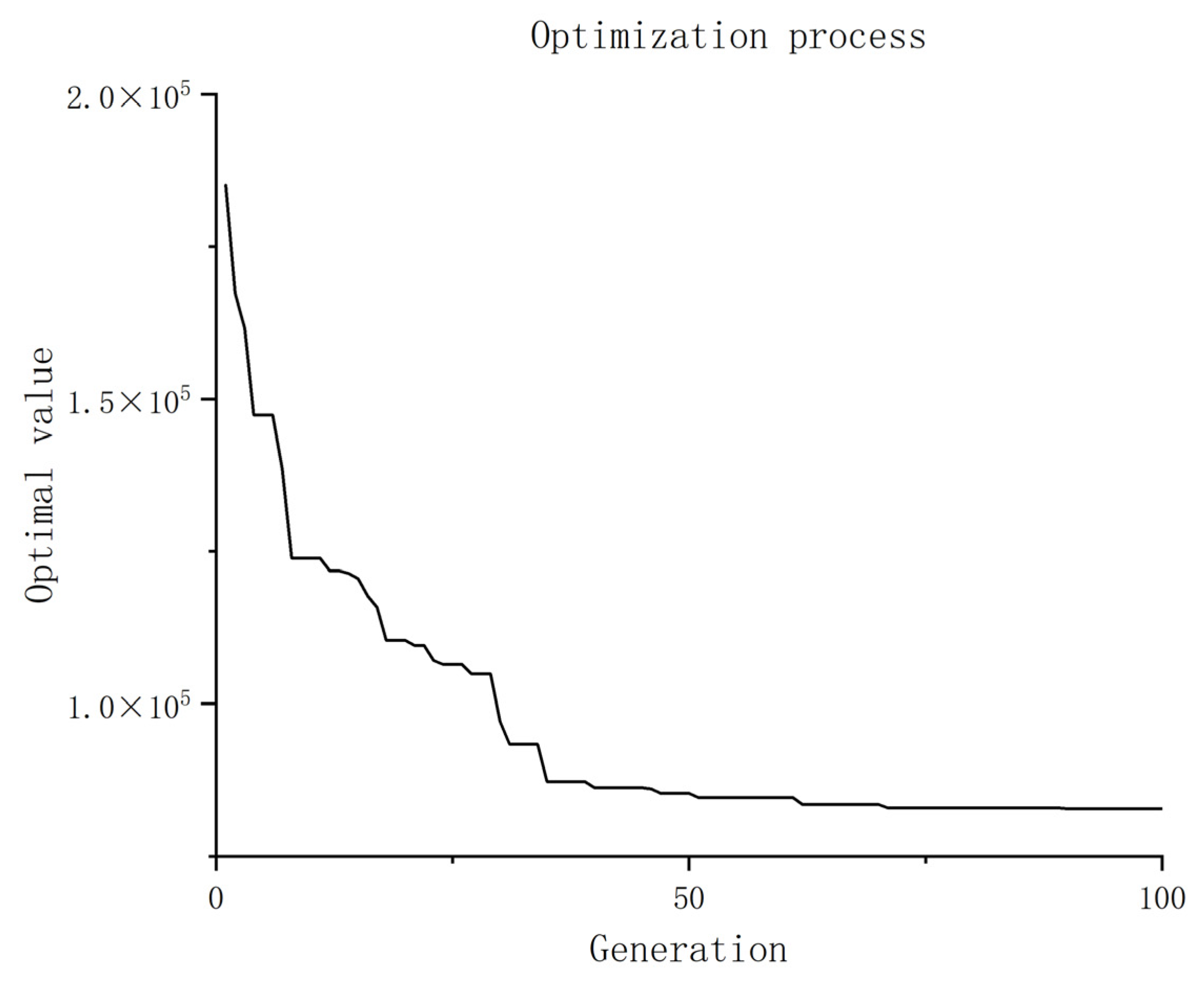
4. Simulation Experiment

4.1. Experimental Setup

To validate the effectiveness of the Improved Genetic Local Search Algorithm with Prior Knowledge (IGLSAPK) proposed in this paper, a simulation experiment was conducted. After 100 iterations of the program, the overall optimal solution was calculated. The parameters for the genetic algorithm were set as follows: a population size of 100, 100 iterations, a crossover probability of 0.9, a mutation probability of 0.05, and a generation gap of 0.9. The chromosome length was set to 200. The decision to iterate 100 times was based on the observation that increasing the iteration count beyond 100 resulted in minimal changes in the optimal value. Considering computational time costs, the iteration count was set to 100. The chromosome length of 200 corresponds to 100 task points and 100 allocation schemes.
To compare the performance of the proposed algorithm, two other algorithms were used for comparison: the Improved Genetic Local Search Algorithm (IGLSA) and the Improved Genetic Algorithm with Priori Knowledge (IGAPK). IGLSA does not have prior knowledge and initialization population algorithms, while IGAPK does not include a local search algorithm, unlike IGLSAPK. The parameters are set the same as before, with 100 iterations.

4.2. Experimental Simulation and Result Analysis

Firstly, we validated the proposed Improved Genetic Local Search Algorithm with Prior Knowledge (IGLSAPK). Within a specified region, 100 task points were randomly generated, and for each task point, task requirements were generated randomly. Each task point set a limit for each of the three types of AUVs, ensuring that the limit for each type could not exceed three vessels. Through simulation experiments, an optimal deployment scheme that minimizes the number of deployments while optimizing overall efficiency was obtained. The final optimal paths meet the requirements of the task points while minimizing overall consumption. The total number of deployments is 5, as shown in the table below Table 1. Notably, during the second and third tasks, two groups are deployed to accomplish the mission.
The overall path is illustrated in Figure 13 (below). It can be observed that, based on the requirements of each task point, all task points are traversed through 5 missions. IGLSAPK simultaneously accomplishes the scheduling and path planning for AUVs, ensuring minimum overall energy consumption. In large-scale problems, precise algorithms often require extensive computation time, and with multiple constraints, the computational workload becomes significantly burdensome, often hindering the rapid acquisition of effective solutions. In the presence of constraints such as AUV-type limitations, quantity restrictions, and on-board energy limitations, where each constraint is coupled with others, the difficulty of solving the problem sharply increases, leading to an exceptionally large computational workload. Heuristic algorithms such as IGLSAPK can rapidly obtain high-quality feasible solutions under these conditions.
Figure 14 depicts the genetic evolution curve over 100 iterations, where the horizontal axis represents the number of iterations, and the vertical axis represents the optimal value for each iteration. With the presence of penalty factors, the initial solutions exhibit higher energy consumption. As the chromosomes undergo iterations, the solutions gradually approach optimality, and around the 100th iteration, the convergence tends to plateau, reaching a relative optimum.

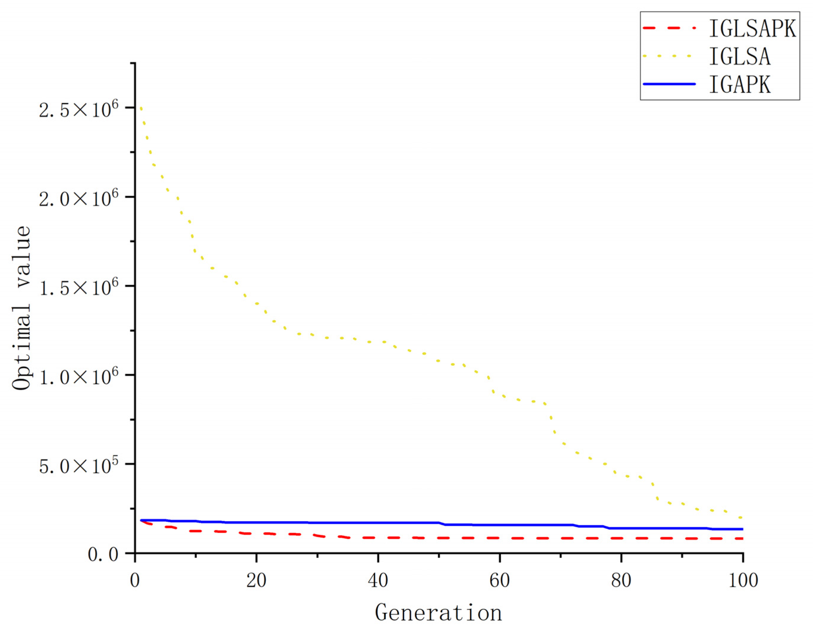
5. Comparative Experiment

To further validate the effectiveness of the proposed IGLSAPK, simulations were conducted separately for IGLSA and IGAPK. To ensure fairness in the experiments, the parameters and initial data were kept consistent with IGLSAPK, and an iteration count of 100 was used. After the simulation experiments, the data were compared and plotted on a single graph (Figure 15).
It can be observed that IGLSA, lacking prior knowledge in generating the initial population and with the presence of penalty factors, started with a very high optimal value. With the assistance of local search algorithms, the optimal value decreased rapidly after multiple iterations. However, it required more iterations to achieve a value close to IGLSAPK. On the other hand, IGAPK, which is without a local search algorithm but benefits from prior knowledge, started with the same optimal value as IGLSAPK. However, the descent of the optimal value was much slower, requiring more iterations to approach the values obtained by IGLSAPK. Additionally, IGAPK was more prone to getting stuck in local optima. Despite this, each iteration ran relatively faster compared to IGLSAPK.
Table 2 reveals that the optimal values obtained with the initial population from prior knowledge were reduced by 91%, 92%, 84%, and 58% in the 25th, 50th, 75th, and 100th iterations, respectively, compared to IGLSA. It indicates that in the early stages where optimal values are relatively small, the efficiency of the solution process is significantly improved. By introducing the local search algorithm, the optimal values decreased by 38%, 49%, 44%, and 38%, respectively, compared to IGAPK. This suggests that the local search algorithm facilitates the rapid convergence of optimal values, greatly enhancing the efficiency of the solution process.

6. Conclusions

This paper addresses the problem of AUV scheduling in underwater docks and proposes the IGLSAPK algorithm. The algorithm tackles the coupled challenges of grouping, task assignment, and path planning for a heterogeneous AUV fleet under complex constraints. Initially, the algorithm introduces a method to convert task point requirements into AUV formation plans. By encoding AUV task points and formation plans simultaneously, the genetic algorithm efficiently addresses both AUV grouping and task assignment. To enhance the algorithm’s efficiency, a knowledge-based initialization algorithm was incorporated, enabling the rapid attainment of low optimal values in the initial iterations. To further improve efficiency and prevent the algorithm from getting trapped in local optima, an enhanced local search algorithm was introduced, significantly boosting the algorithm’s performance. The results of our comparative experiments demonstrate that IGLSAPK outperforms existing genetic algorithms, substantially increasing efficiency. The proposed model is more applicable to real-world scenarios, and the introduced OCEAN matrix can be adjusted based on actual ocean currents, making it more adaptable to real marine environments.
In future research, we will study the AUV swarm scheduling algorithm for multiple underwater docks and investigate the collaborative scheduling algorithm for AUV swarm between surface mother ships and underwater docks.

Author Contributions

Conceptualization, J.W. and T.T.; methodology, J.W.; software, T.T.; validation, J.W., T.T. and R.W.; formal analysis, J.W. and D.L.; investigation, Z.W. and D.L.; data curation, T.T.; writing—original draft preparation, T.T.; writing—review and editing, J.W. and D.L; visualization, T.T.; supervision, J.W.; project administration, J.W. and Z.W.; funding acquisition, D.L. and J.W. All authors have read and agreed to the published version of the manuscript.

Funding

This research is funded by Key Research and Development Program of Jiangsu Province (No. BE2022062).

Institutional Review Board Statement

Not applicable.

Informed Consent Statement

Not applicable.

Data Availability Statement

Data is contained within the article.

Conflicts of Interest

The authors declare no conflict of interest.

References

  1. Li, T.; Sun, S.; Wang, P.; Dong, H.; Wang, X. A Multi-Objective Bi-Level Task Planning Strategy for UUV Target Visitation in Ocean Environment. Ocean Eng. 2023, 288, 116022. [Google Scholar] [CrossRef]
  2. Jin, N. Study on Firefly Algorithm and Its Application in Task Assignment of Multi-AUV System; Harbin Engineering University: Harbin, China, 2016. [Google Scholar]
  3. Zhang, W.; Wang, N.; Wei, S.; Du, X.; Yan, Z. Overview of Unmanned Underwater Vehicle Swarm Development Status and Key Technologies. Harbin Gongcheng Daxue Xuebao/J. Harbin Eng. Univ. 2020, 41, 289–297. [Google Scholar] [CrossRef]
  4. Wang, T.; Lima, R.M.; Giraldi, L.; Knio, O.M. Trajectory Planning for Autonomous Underwater Vehicles in the Presence of Obstacles and a Nonlinear Flow Field Using Mixed Integer Nonlinear Programming. Comput. Oper. Res. 2019, 101, 55–75. [Google Scholar] [CrossRef]
  5. An AUV-Assisted Data Gathering Scheme Based on Clustering and Matrix Completion for Smart Ocean | IEEE Journals & Magazine | IEEE Xplore. Available online: https://ieeexplore.ieee.org/abstract/document/9068243 (accessed on 17 December 2023).
  6. Hao, K.; Zhao, J.; Li, Z.; Liu, Y.; Zhao, L. Dynamic Path Planning of a Three-Dimensional Underwater AUV Based on an Adaptive Genetic Algorithm. Ocean Eng. 2022, 263, 112421. [Google Scholar] [CrossRef]
  7. Che, G.; Liu, L.; Yu, Z. An Improved Ant Colony Optimization Algorithm Based on Particle Swarm Optimization Algorithm for Path Planning of Autonomous Underwater Vehicle. J. Ambient. Intell. Hum. Comput. 2020, 11, 3349–3354. [Google Scholar] [CrossRef]
  8. Mousavian, S.H.; Koofigar, H.R. Identification-Based Robust Motion Control of an AUV: Optimized by Particle Swarm Optimization Algorithm. J. Intell. Robot. Syst. 2017, 85, 331–352. [Google Scholar] [CrossRef]
  9. Chandrawati, T.B.; Sari, R.F. A Review of Firefly Algorithms for Path Planning, Vehicle Routing and Traveling Salesman Problems. In Proceedings of the 2018 2nd International Conference on Electrical Engineering and Informatics (ICon EEI), Batam, Indonesia, 16–17 October 2018; pp. 30–35. [Google Scholar]
  10. Wang, C.; Mei, D.; Wang, Y.; Yu, X.; Sun, W.; Wang, D.; Chen, J. Task Allocation for Multi-AUV System: A Review. Ocean Eng. 2022, 266, 112911. [Google Scholar] [CrossRef]
  11. Polat, K.; Güneş, S. A New Method to Forecast of Escherichia Coli Promoter Gene Sequences: Integrating Feature Selection and Fuzzy-AIRS Classifier System. Expert. Syst. Appl. 2009, 36, 57–64. [Google Scholar] [CrossRef]
  12. Smith, R.G. The Contract Net Protocol: High-Level Communication and Control in a Distributed Problem Solver. IEEE Trans. Comput. 1980, 29, 1104–1113. [Google Scholar] [CrossRef]
  13. Akkiraju, R.; Keskinocak, P.; Murthy, S.; Wu, F. An Agent-Based Approach for Scheduling Multiple Machines. Appl. Intell. 2001, 14, 135–144. [Google Scholar] [CrossRef]
  14. Zhu, D.; Cao, X.; Sun, B.; Luo, C. Biologically Inspired Self-Organizing Map Applied to Task Assignment and Path Planning of an AUV System. IEEE Trans. Cogn. Dev. Syst. 2018, 10, 304–313. [Google Scholar] [CrossRef]
  15. Dechter, R.; Pearl, J. Generalized Best-First Search Strategies and the Optimality of A*. J. ACM 1985, 32, 505–536. [Google Scholar] [CrossRef]
  16. Yan, S.; Pan, F. Research on Route Planning of AUV Based on Genetic Algorithms. In Proceedings of the 2019 IEEE International Conference on Unmanned Systems and Artificial Intelligence (ICUSAI), Xi’an, China, 22–24 November 2019; pp. 184–187. [Google Scholar]
  17. Zhang, Q. A Hierarchical Global Path Planning Approach for AUV Based on Genetic Algorithm. In Proceedings of the 2006 International Conference on Mechatronics and Automation, Luoyang, China, 25–28 June 2006; pp. 1745–1750. [Google Scholar]
  18. Naeem, W.; Sutton, R.; Chudley, J.; Dalgleish, F.R.; Tetlow, S. A Genetic Algorithm-Based Model Predictive Control Autopilot Design and Its Implementation in an Autonomous Underwater Vehicle. Proc. Inst. Mech. Eng. Part M J. Eng. Marit. Environ. 2004, 218, 175–188. [Google Scholar] [CrossRef]
  19. Herlambang, T.; Rahmalia, D.; Yulianto, T. Particle Swarm Optimization (PSO) and Ant Colony Optimization (ACO) for Optimizing PID Parameters on Autonomous Underwater Vehicle (AUV) Control System. J. Phys. Conf. Ser. 2019, 1211, 012039. [Google Scholar] [CrossRef]
  20. Wang, H.; Xiong, W. Research on Global Path Planning Based on Ant Colony Optimization for AUV. J. Marine. Sci. Appl. 2009, 8, 58–64. [Google Scholar] [CrossRef]
  21. Yu, X.; Chen, W.-N.; Gu, T.; Yuan, H.; Zhang, H.; Zhang, J. ACO-A*: Ant Colony Optimization Plus A* for 3-D Traveling in Environments With Dense Obstacles. IEEE Trans. Evol. Computat. 2019, 23, 617–631. [Google Scholar] [CrossRef]
  22. Ma, Y.-N.; Gong, Y.-J.; Xiao, C.-F.; Gao, Y.; Zhang, J. Path Planning for Autonomous Underwater Vehicles: An Ant Colony Algorithm Incorporating Alarm Pheromone. IEEE Trans. Veh. Technol. 2019, 68, 141–154. [Google Scholar] [CrossRef]
  23. Li, Z.; Liu, W.; Gao, L.-E.; Li, L.; Zhang, F. Path Planning Method for AUV Docking Based on Adaptive Quantum-Behaved Particle Swarm Optimization. IEEE Access 2019, 7, 78665–78674. [Google Scholar] [CrossRef]
  24. Wang, L.; Liu, L.; Qi, J.; Peng, W. Improved Quantum Particle Swarm Optimization Algorithm for Offline Path Planning in AUVs. IEEE Access 2020, 8, 143397–143411. [Google Scholar] [CrossRef]
  25. MahmoudZadeh, S.; Powers, D.M.W.; Yazdani, A.M.; Sammut, K.; Atyabi, A. Efficient AUV Path Planning in Time-Variant Underwater Environment Using Differential Evolution Algorithm. J. Marine. Sci. Appl. 2018, 17, 585–591. [Google Scholar] [CrossRef]
  26. Zhang, J.; Liu, M.; Zhang, S.; Zheng, R. AUV Path Planning Based on Differential Evolution with Environment Prediction. J. Intell. Robot. Syst. 2022, 104, 23. [Google Scholar] [CrossRef]
  27. Li, J.; Zhang, R.B. Multi-Auv Distributed Task Allocation Based on the Differential Evolution Quantum Bee Colony Optimization Algorithm. Pol. Marit. Res. 2017, 24, 65–71. [Google Scholar] [CrossRef]
  28. Cai, K.; Wang, C.; Cheng, J.; De Silva, C.W.; Meng, M.Q.-H. Mobile Robot Path Planning in Dynamic Environments: A Survey. arXiv 2021, arXiv:2006.14195. [Google Scholar]
  29. Mac, T.T.; Copot, C.; Tran, D.T.; Keyser, R.D. Heuristic Approaches in Robot Path Planning: A Survey. Robot. Auton. Syst. 2016, 86, 13–28. [Google Scholar] [CrossRef]
  30. Sans-Muntadas, A.; Kelasidi, E.; Pettersen, K.Y.; Brekke, E. Learning an AUV Docking Maneuver with a Convolutional Neural Network. IFAC J. Syst. Control 2019, 8, 100049. [Google Scholar] [CrossRef]
  31. Fujii, T.; Ura, T. Neural-Network-Based Adaptive Control Systems for AUVs. Eng. Appl. Artif. Intell. 1991, 4, 309–318. [Google Scholar] [CrossRef]
  32. Fang, Y.; Huang, Z.; Pu, J.; Zhang, J. AUV Position Tracking and Trajectory Control Based on Fast-Deployed Deep Reinforcement Learning Method. Ocean Eng. 2022, 245, 110452. [Google Scholar] [CrossRef]
  33. Duan, K.; Fong, S.; Chen, C.L.P. Reinforcement Learning Based Model-Free Optimized Trajectory Tracking Strategy Design for an AUV. Neurocomputing 2022, 469, 289–297. [Google Scholar] [CrossRef]
  34. Cao, X.; Sun, C.; Yan, M. Target Search Control of AUV in Underwater Environment With Deep Reinforcement Learning. IEEE Access 2019, 7, 96549–96559. [Google Scholar] [CrossRef]
  35. Wu, H.; Song, S.; Hsu, Y.; You, K.; Wu, C. End-to-End Sensorimotor Control Problems of AUVs with Deep Reinforcement Learning. In Proceedings of the 2019 IEEE/RSJ International Conference on Intelligent Robots and Systems (IROS), Macau, China, 3–8 November 2019; pp. 5869–5874. [Google Scholar]
  36. Carlucho, I.; De Paula, M.; Wang, S.; Petillot, Y.; Acosta, G.G. Adaptive Low-Level Control of Autonomous Underwater Vehicles Using Deep Reinforcement Learning. Robot. Auton. Syst. 2018, 107, 71–86. [Google Scholar] [CrossRef]
  37. Cheng, C.; Sha, Q.; He, B.; Li, G. Path Planning and Obstacle Avoidance for AUV: A Review. Ocean Eng. 2021, 235, 109355. [Google Scholar] [CrossRef]
  38. Nelson, A.L.; Barlow, G.J.; Doitsidis, L. Fitness Functions in Evolutionary Robotics: A Survey and Analysis. Robot. Auton. Syst. 2009, 57, 345–370. [Google Scholar] [CrossRef]
  39. Nanakorn, P.; Meesomklin, K. An Adaptive Penalty Function in Genetic Algorithms for Structural Design Optimization. Comput. Struct. 2001, 79, 2527–2539. [Google Scholar] [CrossRef]
  40. Arram, A.; Ayob, M. A Novel Multi-Parent Order Crossover in Genetic Algorithm for Combinatorial Optimization Problems. Comput. Ind. Eng. 2019, 133, 267–274. [Google Scholar] [CrossRef]
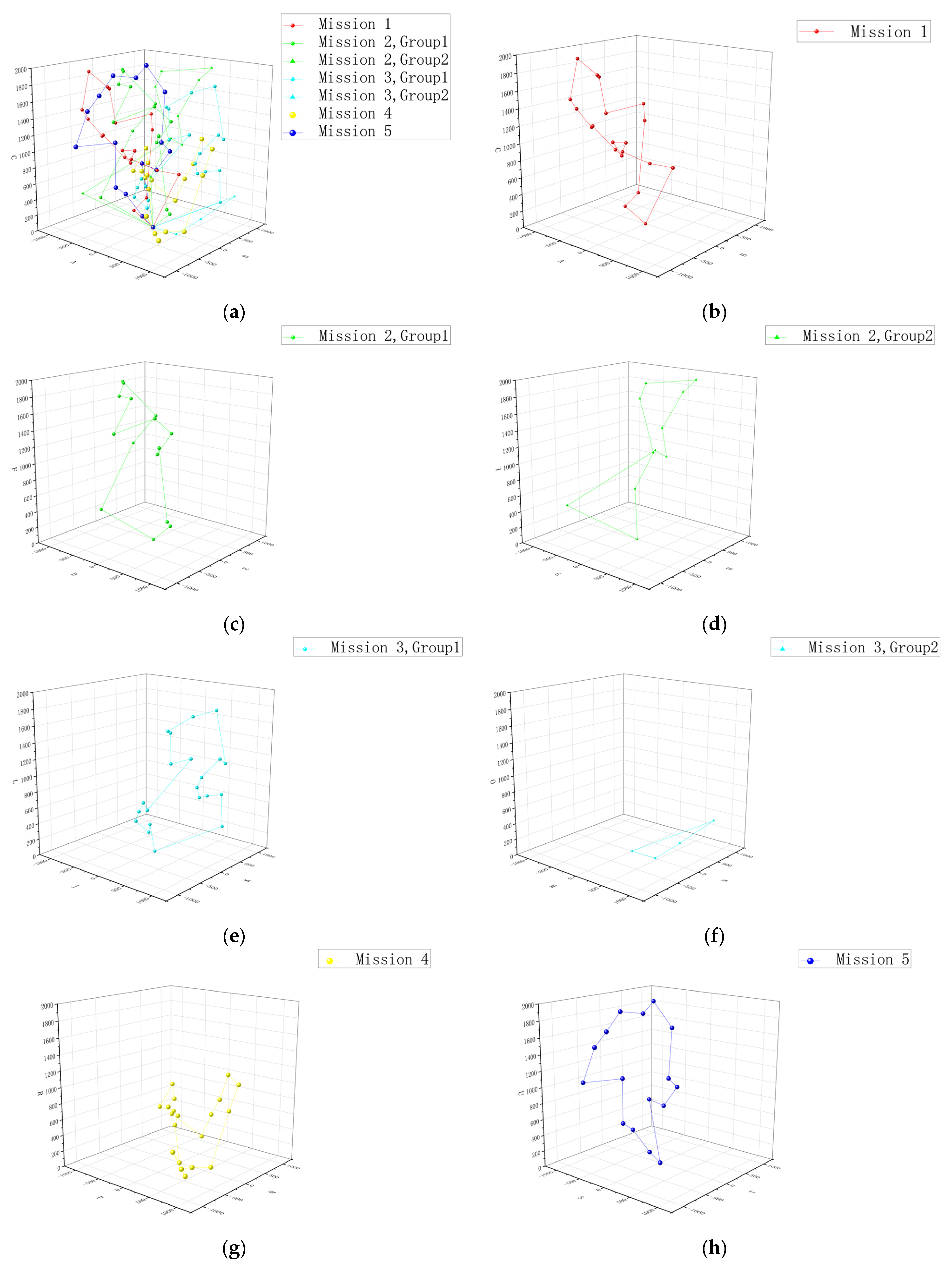
Figure 1. There are multiple task points, each specifying the type and quantity of AUVs required. With several AUVs available, the task is to group these AUVs and then complete the respective tasks.
Jmse 12 00162 g001
Figure 2. After grouping the AUVs, each task point has specific requirements for the quantity and models of AUVs. How do we allocate the task points to AUV groups that meet their requirements?
Jmse 12 00162 g002
Figure 3. Path planning for AUV groups.
Jmse 12 00162 g003
Figure 4. Complete all tasks with minimum total consumption.
Jmse 12 00162 g004
Figure 5. There are multiple task points in a water area, and there is an underwater dock in the middle of the sea. Inside the dock, there are multiple AUVs. These AUVs will form a fleet to navigate to the task points and complete all the tasks.
Jmse 12 00162 g005
Figure 6. A diagram of an underwater dock allowing for AUV energy replenishment and information exchange.
Jmse 12 00162 g006
Figure 7. Complete flowchart of the algorithm’s process. Where G is the designated number of iterations, and the iteration starts from 1, concluding when the count reaches G.
Jmse 12 00162 g007
Figure 8. Partial task demands chart including three-dimensional coordinates and quantity requirements for various types of AUVs.
Jmse 12 00162 g008
Figure 9. Adopting the bubble sort algorithm to process data based on prior knowledge.
Jmse 12 00162 g009
Figure 10. Randomly generate 100 task points, each comprising a serial number, three-dimensional coordinates, and quantity requirements for 3 types of AUVs.
Jmse 12 00162 g010
Figure 11. The 100 corresponding grouping plans, including the quantity of each type of AUV.
Jmse 12 00162 g011
Figure 12. Randomly select two parent individuals as the crossover objects. Choose a random substring from the first parent individual and copy it to the corresponding position in the offspring individual. Based on the order in the second parent individual, copy the remaining genes to the offspring individual in the order of the unselected genes, ensuring that each gene is non-repetitive.
Jmse 12 00162 g012
Figure 13. (a) The route map for all tasks; (b) the route map for Task 1; (c) the route map for Task 2, Group 1; (d) the route map for Task 2, Group 2; (e) the route map for Task 3, Group 1; (f) the route map for Task 3, Group 2; (g) the route map for Task 4; (h) the route map for Task 5.
Jmse 12 00162 g013
Figure 14. Iteration 100 times, where the horizontal axis represents the number of iterations, and the vertical axis represents the optimal value.
Jmse 12 00162 g014
Figure 15. Comparison graph of IGLSAPK, IGLSA, and IGAPK algorithms after 100 iterations, where the horizontal axis represents the number of iterations, and the vertical axis represents the optimal value.
Jmse 12 00162 g015
Table 1. Illustrative table of AUV group paths.
MissionGroupRouteScheme NumberScheme
Mission1Group10 → 4 → 64 → 66 → 8 → 94 → 14 → 69 → 24 → 2 → 25 → 100 → 43 → 49 → 95 → 28 → 29 → 42 → 52 → 15 → 0102A3B3C3
Mission2Group10 → 45 → 87 → 98 → 90 → 61 → 31 → 73 → 62 → 97 → 47 → 46 → 63 → 13 → 71 → 0112A2B2C3
Group20 → 83 → 40 → 70 → 56 → 50 → 37 → 3 → 38 → 33 → 57 → 9 → 17 → 68 → 89 → 86 → 0103A3B3C2
Mission3Group10 → 39 → 75 → 84 → 99 → 58 → 92 → 77 → 36 → 81 → 55 → 0125A2B2C2
Group20 → 32 → 34 → 54 → 0108A3B2C3
Mission4Group10 → 74 → 80 → 72 → 5 → 59 → 18 → 53 → 10 → 6 → 19 → 51 → 65 → 85 → 44 → 67 → 20 → 48 → 76 → 91 → 93 → 0105A3B2C3
Mission5Group10 → 23 → 60 → 11 → 26 → 1 → 7 → 21 → 41 → 88 → 79 → 22 → 96 → 30 → 27 → 35 → 12 → 82 → 16 → 78 → 0101A3B3C3
Table 2. A table comparing the optimal values for the IGLSAPK, IGLSA, and IGAPK algorithms at the 25th, 50th, 75th, and 100th iterations.
AlgorithmNumber of Iterations
255075100
IGLSAPK106,482.5085,298.3482,935.1982,768.82
IGLSA1,250,001.211,080,032.35530,031.92200,031.78
IGAPK173,131.74170,121.81150,023.62135,021.43
Disclaimer/Publisher’s Note: The statements, opinions and data contained in all publications are solely those of the individual author(s) and contributor(s) and not of MDPI and/or the editor(s). MDPI and/or the editor(s) disclaim responsibility for any injury to people or property resulting from any ideas, methods, instructions or products referred to in the content.

